Photonic crystals in technology
8
DPMS Ad dMt il DPMS: AdvancedMaterials Lecture E11: Computational Optics II Elefterios Lidorikis Room Π1 26510 07146 Room Π1, 26510 07146 [email protected] http://cmsl.materials.uoi.gr/lidorikis Photonic crystals in technology • Applications in extreme light manipulation 2 Plasmonics in technology + + + + Localized Plasmons localized surface plasmon resonance (LSPR) Propagating Plasmons surface plasmon polariton (SPP) + + + + + + + + + + + + + + + + + + + + + + + + + + + + + + ‐ ‐ ‐ ‐ ‐ ‐ ‐ ‐ ‐ ‐ ‐ ‐ ‐ ‐ ‐ ‐ ‐ ‐ ‐ ‐ ‐ ‐ + + + + + + + + + + + + + + + + + + + + + + + + + + + + + + ‐ ‐ ‐ ‐ ‐ ‐ ‐ ‐ ‐ ‐ ‐ ‐ ‐ ‐ ‐ ‐ ‐ ‐ ‐ ‐ ‐ ‐ ‐ ‐ ‐ ‐ ‐ ‐ + + ‐ ‐ kondinski.webs.com Numerical solutions in photonics • Time domain – direct time integration of Maxwell’s equations i t l th fi it diff ti d i (FDTD) th d – main tool the finite‐difference time‐domain (FDTD) method – frequency information obtained by Fourier transform of the time evolution • Frequency domain – eigenvalue solutions – plane‐wave expansion method, finite element method, transfer matrix method – time domain information by solution superposition
Transcript of Photonic crystals in technology
DPMS Ad d M t i lDPMS: Advanced Materials
Lecture E11: Computational Optics II
Elefterios LidorikisRoom Π1 26510 07146Room Π1, 26510 [email protected]://cmsl.materials.uoi.gr/lidorikis
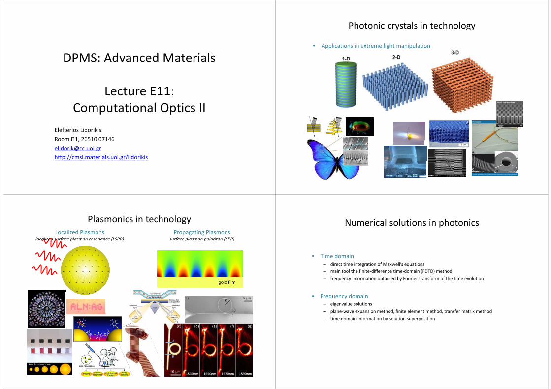
Photonic crystals in technology
• Applications in extreme light manipulation
2
Plasmonics in technology
+ + ++
Localized Plasmonslocalized surface plasmon resonance (LSPR)
Propagating Plasmonssurface plasmon polariton (SPP)
+ + ++ +++ + ++ ++ ++ + ++ +++ +
+ ++ +++ + ++
‐ ‐ ‐‐ ‐‐‐ ‐ ‐‐ ‐‐ ‐
‐ ‐‐ ‐‐‐ ‐ ‐‐
+ + ++ ++ ++ + ++ +++ ++ ++
+ + ++ +++ +
+ + ++
‐ ‐ ‐‐ ‐‐ ‐‐ ‐ ‐‐ ‐‐‐ ‐‐ ‐‐
‐ ‐ ‐‐ ‐‐‐ ‐
‐‐ + +‐ ‐
kondinski.webs.com
Numerical solutions in photonics
• Time domain– direct time integration of Maxwell’s equations
i t l th fi it diff ti d i (FDTD) th d– main tool the finite‐difference time‐domain (FDTD) method– frequency information obtained by Fourier transform of the time evolution
• Frequency domain– eigenvalue solutions– plane‐wave expansion method, finite element method, transfer matrix methodp p , ,– time domain information by solution superposition
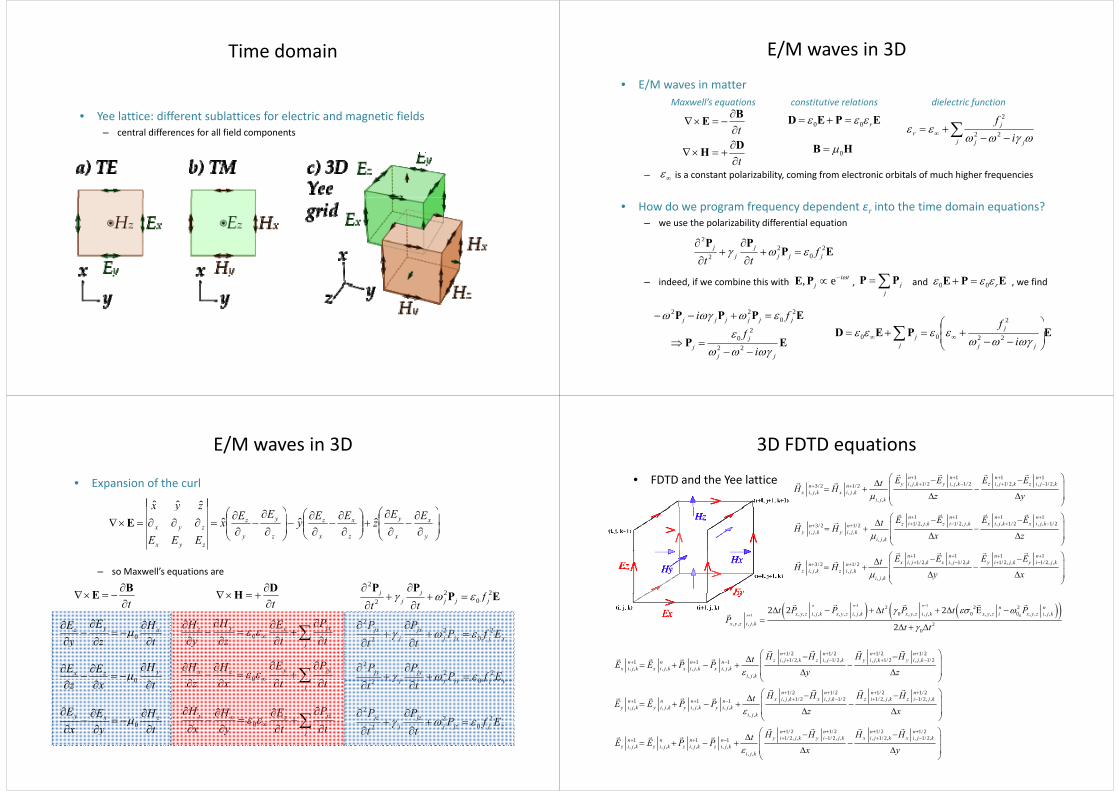
Time domain
l d ff bl f l d f ld• Yee lattice: different sublattices for electric and magnetic fields– central differences for all field components
E/M waves in 3D
• E/M waves in matter
Bconstitutive relationsMaxwell’s equations dielectric function
t
DH
BE EPED r 00
HB 0
j jj
jr i
f
22
2
– is a constant polarizability, coming from electronic orbitals of much higher frequenciest
H 0
• How do we program frequency dependent εr into the time domain equations?– we use the polarizability differential equation
PP2
– indeed, if we combine this with , and , we find
EPPP 2
02
2 jjjj
jj f
tt
tij
e,PE EPE r 00 jPPindeed, if we combine this with , and , we find
EPPP 20
22jjjjjj fi
j, r00j
j
2
jf2
EPjj
jj i
f
22
20 EPED
jj
j
jj i
f
2200
E/M waves in 3D
• Expansion of the curl
zyx ˆˆˆ
y
x
x
y
z
x
x
z
z
y
y
z
zyx
zyxEE
zEEyEEx
EEE
zyxˆˆˆE
– so Maxwell’s equations are
BE DH EP
PP 222
jj f
t E
HEE xyz
0
t H EP 2
02
2 jjjj
jj f
tt
jxxyz PEHH 0 jjj
jxj
jx EfPPP 2
02
2
HEE yzx
0
tzy 0 j ttzy 0
jyyzx PEHH 0
xjjxjj EfPtt 02
yjjyjjy
jjy EfP
PP 20
22
2
txz 0
HEE zxy
0
j ttxz 0
jzzxy PEHH
0
yjjyjj EfPtt 02
jzjz EfPPP 22
2
tyx 0
j ttyx
0 zjjzjj EfPtt 02
3D FDTD equations
• FDTD and the Yee lattice 1 1 1 1, , 1/ 2 , , 1/ 2 , 1/ 2, , 1/ 2,3/ 2 1/ 2
, , , ,, ,
n n n ny i j k y i j k z i j k z i j kn n
x i j k x i j ki j k
E E E EtH Hz y
1 1 1 11/ 2, , 1/ 2, , , , 1/ 2 , , 1/ 23/ 2 1/ 2
, , , ,, ,
n n n nz i j k z i j k x i j k x i j kn n
y i j k y i j ki j k
E E E EtH Hx z
1 1 1 1, 1/ 2, , 1/ 2, 1/ 2, , 1/ 2, ,3/ 2 1/ 2
, , , ,, ,
n n n nx i j k x i j k y i j k y i j kn n
z i j k z i j ki j k
E E E EtH Hy x
1 1
1 0
2 2 2, , , , , , , , 0 , , , , 0 , , 0 , , , ,
, , , , 20
2 2 2
2
n n n
n
n nx y z i j k x y z i j k x y z i j k x y z i x y z i j k
x y z i j k
t P P t P t PP
t t
1/ 2 1/ 2 1/ 2 1/ 2, 1/ 2, , 1/ 2, , , 1/ 2 , , 1/ 21 1 1
, , , , , , , ,, ,
n n n nz i j k z i j k y i j k y i j kn n n n
x i j k x i j k x i j k x i j ki j k
H H H HtE E P Py z
1/ 2 1/ 2 1/ 2 1/ 2
, , 1/ 2 , , 1/ 2 1/ 2, , 1/ 2, ,1 1 1, , , , , , , ,
, ,
n n n nx i j k x i j k z i j k z i j kn n n n
y i j k y i j k y i j k y i j ki j k
H H H HtE E P Pz x
1/ 2 1/ 2 1/ 2 1/ 21/ 2, , 1/ 2, , , 1/ 2, , 1/ 2,1 1 1
, , , , , , , ,, ,
n n n ny i j k y i j k x i j k x i j kn n n n
z i j k z i j k z i j k z i j ki j k
H H H HtE E P Px y
Frequency domain
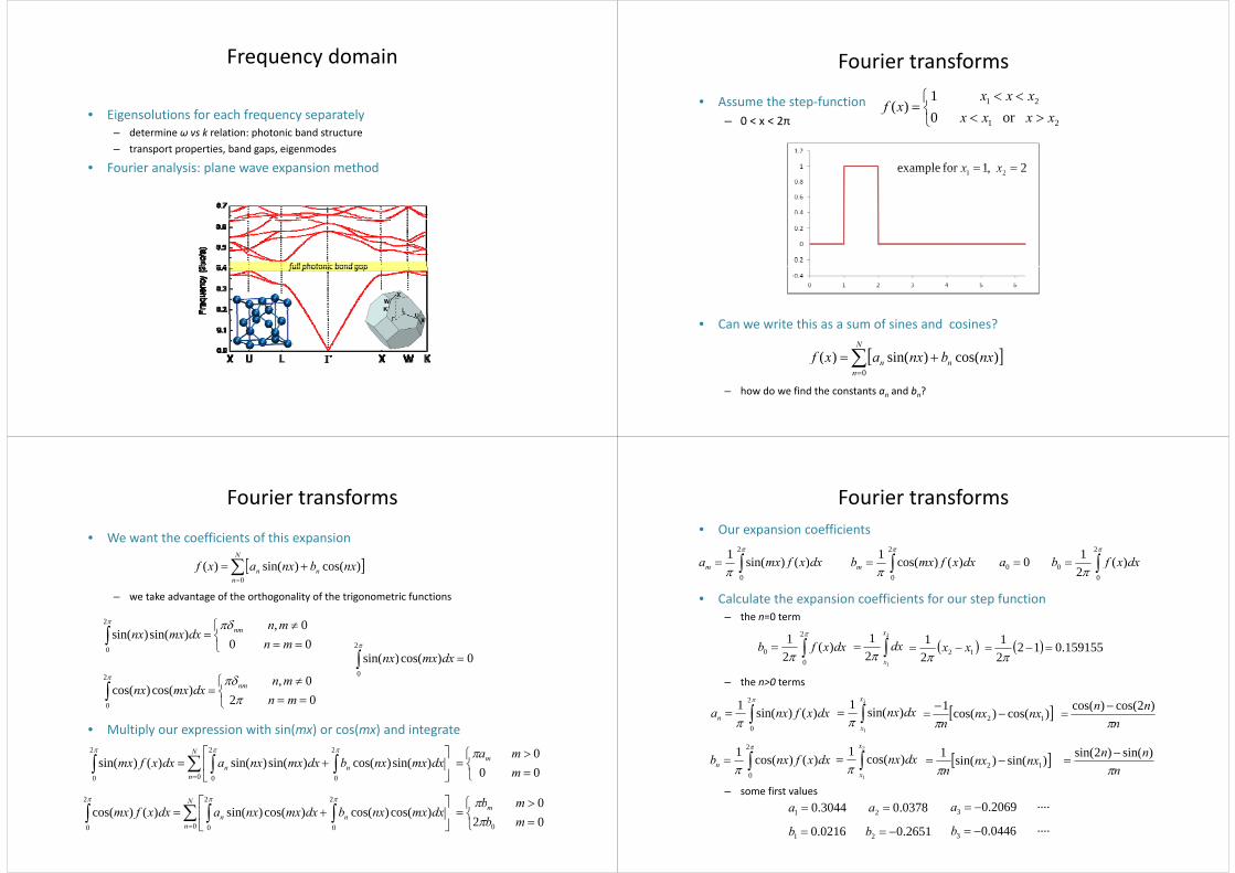
• Eigensolutions for each frequency separately – determine ω vs k relation: photonic band structure– transport properties, band gaps, eigenmodes
• Fourier analysis: plane wave expansion methodFourier analysis: plane wave expansion method
Fourier transforms
• Assume the step‐function– 0 < x < 2π
21
21
or 01
)(xxxx
xxxxf
0 < x < 2π 21
2,1forexample 21 xx 2 ,1for example 21 xx
• Can we write this as a sum of sines and cosines?
N
nn nxbnxaxf )cos()sin()(
– how do we find the constants an and bn?
n
nnf0
)()()(
Fourier transforms
• We want the coefficients of this expansion
N
– we take advantage of the orthogonality of the trigonometric functions
n
nn nxbnxaxf0
)cos()sin()(
00,
0)sin()sin(
2
0
mnmn
dxmxnx nm
0)()i (2
d 0)cos()sin(0
dxmxnx
00,
2)cos()cos(
2
mnmn
dxmxnx nm
• Multiply our expression with sin(mx) or cos(mx) and integrate
020 mn
N 222 0
N
nnn dxmxnxbdxmxnxadxxfmx
0
2
0
2
0
2
0
)sin()cos()sin()sin()()sin(
00
0
mmam
222 0 b
N
nnn dxmxnxbdxmxnxadxxfmx
0
2
0
2
0
2
0
)cos()cos()cos()sin()()cos(
00
2 0
mm
bbm
Fourier transforms• Our expansion coefficients
2
)()i (1 df 2
)()(1 dfb 2
)(1 dfb0
• Calculate the expansion coefficients for our step function
0
)()sin( dxxfmxam 0
)()cos( dxxfmxbm 0
0 )(2
dxxfb00 a
– the n=0 term
2
0 )(21 dxxfb
2
21 x
dx
159155.01221
1221 xx
– the n>0 terms
02
21 21 x
1
2 x
2
2
1 )2()(
0
)()sin(1 dxxfnxan 2
1
)sin(1
x
dxnx
)cos()cos(112 nxnx
n
21 21 x1
nnn
)2cos()cos(
)i ()2i (
– some first values
0
)()cos(1 dxxfnxbn 1
)cos(1
x
dxnx
)sin()sin(112 nxnx
n
nnn
)sin()2sin(
3044.01 a 0378.02 a 2069.03 a ....
0216.01 b 2651.02 b 0446.03 b ....
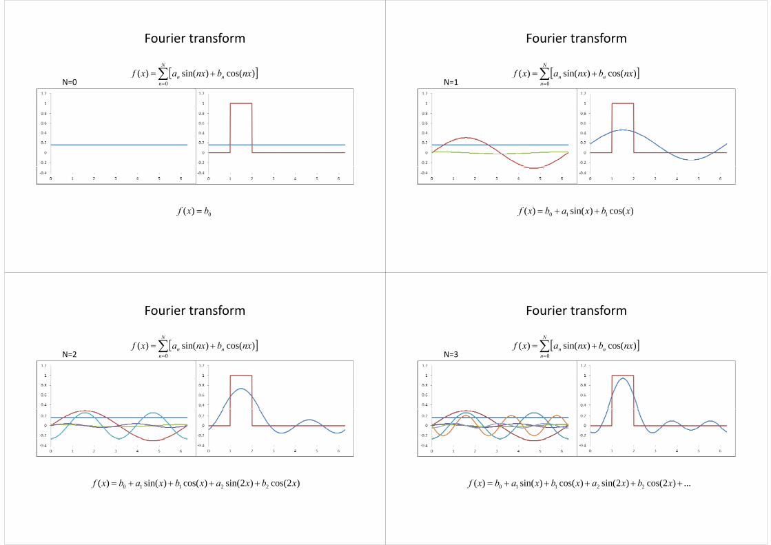
Fourier transform
N
nn nxbnxaxf )cos()sin()(N=0
n
nnf0
)()()(
0)( bxf
Fourier transform
N
nn nxbnxaxf )cos()sin()(N=1
n
nnf0
)()()(
)cos()sin()( 110 xbxabxf
Fourier transform
N
nn nxbnxaxf )cos()sin()(N=2
n
nnf0
)()()(
)2cos()2sin()cos()sin()( 22110 xbxaxbxabxf
Fourier transform
N
nn nxbnxaxf )cos()sin()(N=3
n
nnf0
)()()(
...)2cos()2sin()cos()sin()( 22110 xbxaxbxabxf
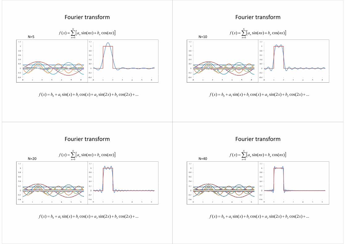
Fourier transform
N
nn nxbnxaxf )cos()sin()(N=5
n
nnf0
)()()(
...)2cos()2sin()cos()sin()( 22110 xbxaxbxabxf
Fourier transform
N
nn nxbnxaxf )cos()sin()(N=10
n
nnf0
)()()(
...)2cos()2sin()cos()sin()( 22110 xbxaxbxabxf
Fourier transform
N
nn nxbnxaxf )cos()sin()(N=20
n
nnf0
)()()(
...)2cos()2sin()cos()sin()( 22110 xbxaxbxabxf
Fourier transform
N
nn nxbnxaxf )cos()sin()(N=40
n
nnf0
)()()(
...)2cos()2sin()cos()sin()( 22110 xbxaxbxabxf
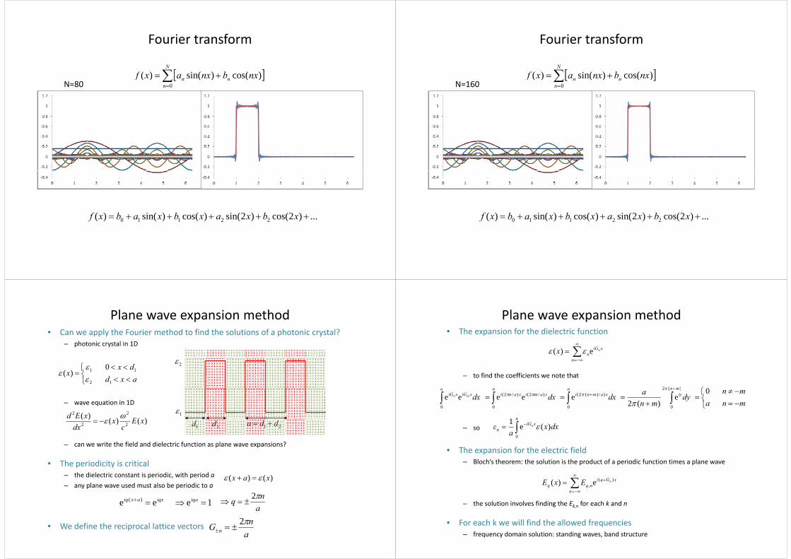
Fourier transform
N
nn nxbnxaxf )cos()sin()(N=80
n
nnf0
)()()(
...)2cos()2sin()cos()sin()( 22110 xbxaxbxabxf
Fourier transform
N
nn nxbnxaxf )cos()sin()(N=160
n
nnf0
)()()(
...)2cos()2sin()cos()sin()( 22110 xbxaxbxabxf
Plane wave expansion method• Can we apply the Fourier method to find the solutions of a photonic crystal?
– photonic crystal in 1D
axddx
x1
1
2
1 0)(
2
– wave equation in 1D1
)()()( 22
ExEd
– can we write the field and dielectric function as plane wave expansions?
1d 2d 21 dda )()()(22 xEc
xdx
• The periodicity is critical– the dielectric constant is periodic, with period a )()( xax – any plane wave used must also be periodic to a
)()(
iqxaxiq ee )( 1e iqa
anq 2
• We define the reciprocal lattice vectorsanG n2
Plane wave expansion method• The expansion for the dielectric function
xiGn
nx e)(
– to find the coefficients we note that
n
a a a )(2 mn 0a
xiGxiG dxmn
0
ee a
xamixani dx0
)/2()/2( ee a
xamni dx0
)/)(2(e
)(2
0
e)(2
mniydy
mna
mnmn
a0
a1– so
• The expansion for the electric field
a
0
)(e1 dxxa
ε xiGn
n
• The expansion for the electric field– Bloch’s theorem: the solution is the product of a periodic function times a plane wave
xGqiEE )()(
– the solution involves finding the Ek,n for each k and n
n
xGqinqq
nExE )(, e)(
• For each k we will find the allowed frequencies– frequency domain solution: standing waves, band structure
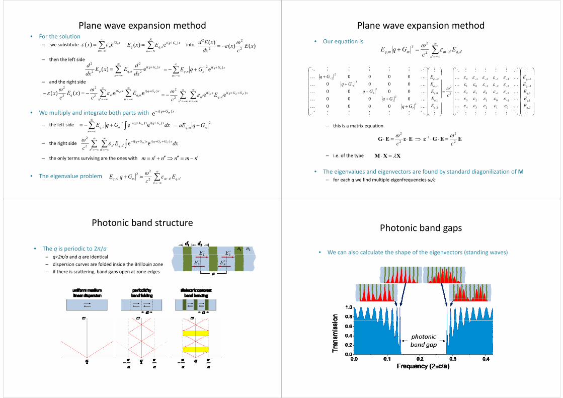
F h l iPlane wave expansion method
• For the solution– we substitute into
n
xiGn
nx e)(
N
Nn
xGqinqq
nExE )(, e)( )()()(
2
2
2
2
xEc
xdxxEd
– then the left side
n
xGqinqq
n
dxdExE
dxd )(
2
2
,2
2
e)(
n
xGqinnq
nGqE )(2, e
– and the right side
n
xGqinq
n
xiGnq
nn Ec
xEc
x )(,2
2
2
2
ee)()(
xGGqinq
xiGn
nnn Ec
)(,2
2
ee
• We multiply and integrate both parts with
nn n nc
2
xGqi m )(e
2– the left side
the right side
2, mmq GqaE
xGGqixGqi dxE nnm )()(2
ee
n
xGqixGqinnq dxGqE nm )()(2
, ee
– the right side
– the only terms surviving are the ones with
n n
nqn dxEc
nnm,2 ee
nmnnnm
• The eigenvalue problem
nnqnmmmq E
cGqE ,2
22
,
Plane wave expansion method• Our equation is
nnqnmmmq E
cGqE ,2
22
, nc
2432102
22 0000 EEGq
1
0,
1,
2,
10123
21012
32101
43210
2
2
1
0,
1,
2,
21
20
21
2
0000000000000000
q
q
q
q
q
q
EEEE
cEEEE
GqGq
GqGq
2,
1,
01234
10123
2,
1,2
2
1
00000000
q
q
q
q
EE
EE
GqGq
– this is a matrix equation
EEGεEεEG 2
21
2
2
cc
– i.e. of the type
cc
XXM
• The eigenvalues and eigenvectors are found by standard diagonilization of M– for each q we find multiple eigenfrequencies ω/c
Photonic band structure
• The q is periodic to 2π/a/ d d l– q+2π/a and q are identical
– dispersion curves are folded inside the Brillouin zone– if there is scattering, band gaps open at zone edges
Photonic band gaps
• We can also calculate the shape of the eigenvectors (standing waves)p g ( g )
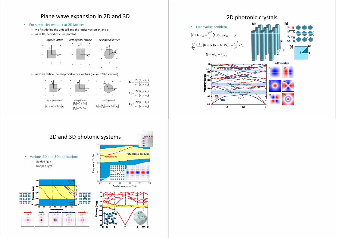
Plane wave expansion in 2D and 3D• For simplicity we look at 2D lattices
– we first define the unit cell and the lattice vectors a1 and a2i 1D i di it i i t t– as in 1D, periodicity is important
square lattice orthogonal lattice hexagonal lattice
– next we define the reciprocal lattice vectors (i.e. our 2D G vectors)
)()(2
321
321 aaa
aab
)( 321
)()(2
321
132 aaa
aab
)()(2
321
213 aaa
aab
2D photonic crystals• Eigenvalue problem
2
G
Ec
E GGGGGk 2
GGGG GkGk HH 2
21
or,
GG
GGG c 2
2211 bbG nn
2D and 3D photonic systemsp y
• Various 2D and 3D applications– Guided light
T d li ht– Trapped light