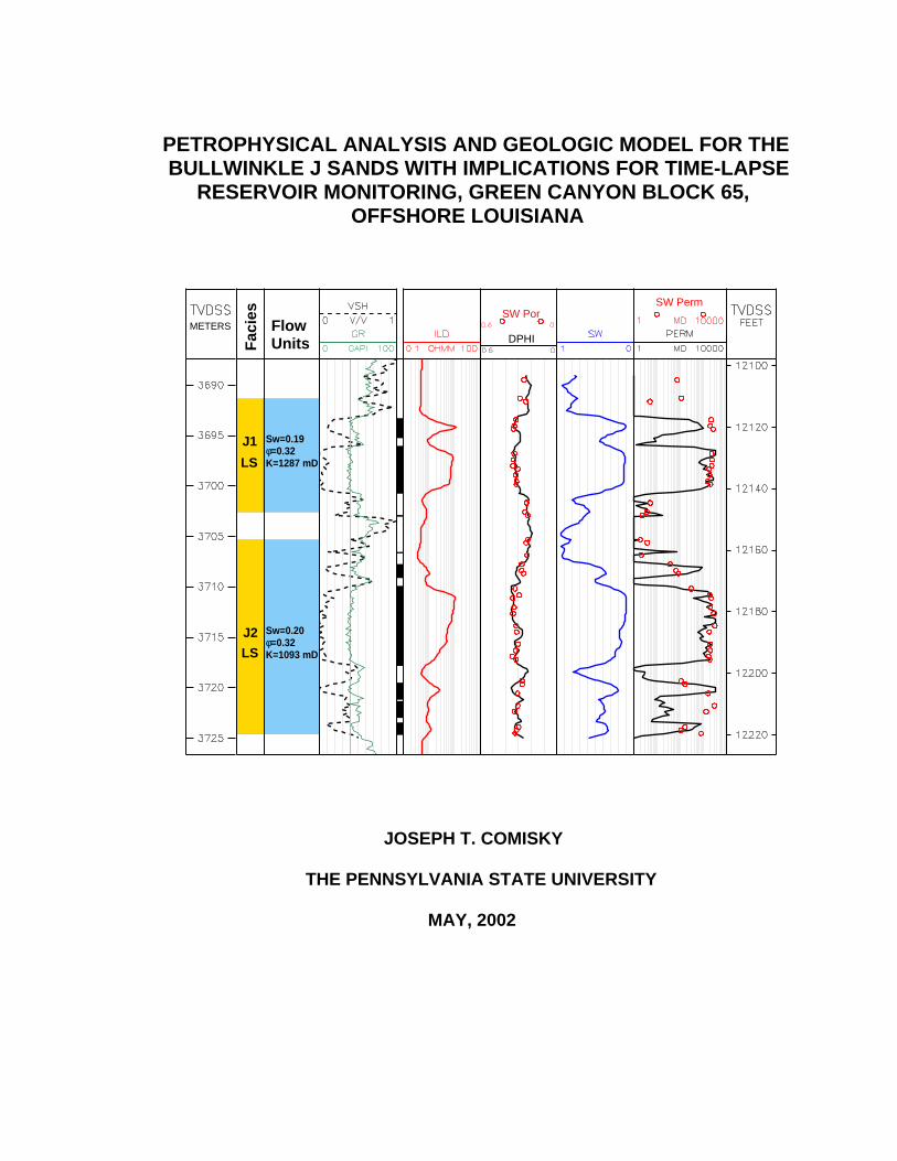
petrophysical analysis and geologic model for the bullwinkle j sands ...

J1

LS

Sw=0.19φ=0.32K=1287 mD

SW Perm

Fac

ies

Flow Units

METERSSW Por

LS

J2

DPHI

Sw=0.20φ=0.32K=1093 mD

PETROPHYSICAL ANALYSIS AND GEOLOGIC MODEL FOR THE BULLWINKLE J SANDS WITH IMPLICATIONS FOR TIME-LAPSE RESERVOIR MONITORING, GREEN CANYON BLOCK 65, OFFSHORE LOUISIANA

JOSEPH T. COMISKY

THE PENNSYLVANIA STATE UNIVERSITY

MAY, 2002

The Pennsylvania State University

The Graduate School

College of Earth and Mineral Sciences

PETROPHYSICAL ANALYSIS AND GEOLOGIC MODEL FOR THE

BULLWINKLE J SANDS WITH IMPLICATIONS FOR TIME-LAPSE

RESERVOIR MONITORING, GREEN CANYON BLOCK 65,

OFFSHORE LOUISIANA

A Thesis inGeosciences

by

Joseph T. Comisky

Copyright 2002 Joseph T. Comisky

Submitted in Partial Fulfillmentof the Requirements

for the Degree of

Master of Science

May 2002

We approve the thesis of Joseph T. Comisky.

Date of Signature

Peter B. FlemingsAssociate Professor of GeosciencesThesis Advisor

Phillip M. HalleckAssociate Professor of Petroleum and Natural Gas Engineering

Chris J. MaroneAssociate Professor of Geosciences

Peter DeinesProfessor of GeochemistryAssociate Head for Graduate Programs and Research

r the

c on

I grant The Pennsylvania State University the non-exclusive right to use this work fo

University’s own purposes and to make single copies of the work available to the publi

a not-for-profit basis if copies are not otherwise available.

Joseph T. Comisky

iii

mbi-

prop-

del to

prop-

ith an

onal

d J2

cut

es

ater

f the

1997

ctual

by

as-

much

e

peri-

ubble

cient

Abstract

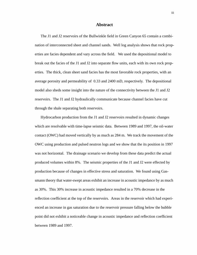
The J1 and J2 reservoirs of the Bullwinkle field in Green Canyon 65 contain a co

nation of interconnected sheet and channel sands. Well log analysis shows that rock

erties are facies dependent and vary across the field. We used the depositional mo

break out the facies of the J1 and J2 into separate flow units, each with its own rock

erties. The thick, clean sheet sand facies has the most favorable rock properties, w

average porosity and permeability of 0.33 and 2400 mD, respectively. The depositi

model also sheds some insight into the nature of the connectivity between the J1 an

reservoirs. The J1 and J2 hydraulically communicate because channel facies have

through the shale separating both reservoirs.

Hydrocarbon production from the J1 and J2 reservoirs resulted in dynamic chang

which are resolvable with time-lapse seismic data. Between 1989 and 1997, the oil-w

contact (OWC) had moved vertically by as much as 284 m. We track the movement o

OWC using production and pulsed neutron logs and we show that the its position in

was not horizontal. The drainage scenario we develop from these data predict the a

produced volumes within 8%. The seismic properties of the J1 and J2 were effected

production because of changes in effective stress and saturation. We found using G

smann theory that water-swept areas exhibit an increase in acoustic impedance by as

as 30%. This 30% increase in acoustic impedance resulted in a 70% decrease in th

reflection coefficient at the top of the reservoirs. Areas in the reservoir which had ex

enced an increase in gas saturation due to the reservoir pressure falling below the b

point did not exhibit a noticeable change in acoustic impedance and reflection coeffi

between 1989 and 1997.

iv

Table of Contents

List of Figures vi

List of Tables xi

Acknowledgements xii

Chapter 1. INTRODUCTION 1

References 4

Chapter 2. FORMATION EVALUATION AND DEPOSITIONAL MODELFOR THE BULLWINKLE J SANDS, GREEN CANYON BLOCK

65, OFFSHORE LOUISIANA

6

Abstract 6

Introduction 6

Formation Evaluation 11

Porosity 11

Water Saturation 21

Permeability 29

Geologic Model 36

Facies and Depositional Environments 36

Amalgamated Sheet Sand 36

Layered Sheet Sand 36

Channel Sand 40

Levee 42

Geologic Evolution 42

Implications for Production and Sand Connectivity 44

Comparison with Other Deepwater Gulf of Mexico Fields 45

Flow Units 47

Conclusions 56

References 57

Nomenclature 60

Chapter 3. RESERVOIR MONITORING OF THE BULLWINKLE J SANDSUSING PRODUCTION DATA, PULSED NEUTRON LOGS,AND GASSMANN FLUID SUBSTITUTION MODELING WITHCOPMARISON TO TIME-LAPSE SEISMIC RESULTS, GREENCANYON BLOCK 65, OFFSHORE LOUISIANA

66

v

2

2

Abstract 66

Introduction 67

Production Characterization 69

J1 and J2 Initial Volumes 69

Drainage Analysis 72

OWC Movement: 1989-1992 78






General OWC Behavior 83

J1 and J2 Volumes, 1997 83

Drained Pay Volumes for the J1 and J2 87

Gassmann Model 92

Porosity, Effective Stress, and Vp Observations 95

Porosity, Effective Stress, and Kdry Observations 97

Effective Stress/Kdry Model 99

Velocity Model for Water-Saturated Rocks Under Pressure 10

Saturation Effects on Velocity and Amplitude 104

Coupled Pressure and Saturation Effects on the Acoustic Properties

107

Model of Acoustic Response Due to Water Sweep andChanges in Effective Stress

107

Modeling of Gas Exsolution and Effective Stress Changes 11

Summary of Gassmann Model 115

Conclusions 120

Nomenclature 121

References 126

Appendix A. PNC Log Methodology 129

References 132

Appendix B. Gassmann Model Outputs 133

vi

List of Figures

2.1 Bathymetric map showing the Gulf of Mexico and the BullwinkleField

7

2.2 J1 Structure map 9

2.3 J2 Structure map 10

2.4 Summary description of several types of turbidite reservoirs commonto the Gulf of Mexico

12

2.5 Type well log responses and whole core-measured porosities from theA32 BP well showing GR, ILD, NPHI, and RHOB

14

2.6 Crossplot of DPHI vs. whole core-measured porosites from the A32BP in the J3 Sand

15

2.7 Crossplot of DPHI vs. whole core-measured porosities from the J1and J2 sands in the A32 BP.

(a) DPHI vs. whole core data plotted from 0 to 1(b) DPHI vs. whole core data plotted only in the dashed area ofFigure 2.7a

16

2.8 Well log responses from the 65-1 18

2.9 DPHI vs. sidewall core porosities in oil and gas zones of the 65-1well

20

2.10 Well log responses from the A36 well in the J2 showing how F wascalculated from the ILD log.

23

2.11 Log-log plot of F vs.φ for the whole core data presented in Table 2.2and well log data from the A-36.

24

2.12 Log-log plot of Sw vs. I using the whole core data presented in Tables2.3 and 2.4

26

2.13 Pickett plot of resistivity data 28

2.14 Predicted Sw vs. measured Sw when a=0.72, n=1.85, and m=2.03 30

2.15 Semi-log crossplot of whole core measured K vs.φ for the A32 BPand 65-1 wells

32

vii

39

41

2.16 Crossplot of predicted K vs. measured K using whole core data fromthe A32 BP

34

2.17 Permeability transform presented in Equation 9 derived from stressedwhole core data from the A32 BP

(a) Permeability transform plotted with whole core data from theA32 BP(b) Permeability transform plotted with stressed whole core datafrom the A32 BP showing the dependence of K onφ for constantVsh

35

2.18 Type well log responses and facies map for the J2 sand(a) Type log response for the AS facies(b) Facies map of the J2 sand(c) Type log response for the LS facies(d) Type well log response for the CS facies(e) Type well log response for the LV facies

37

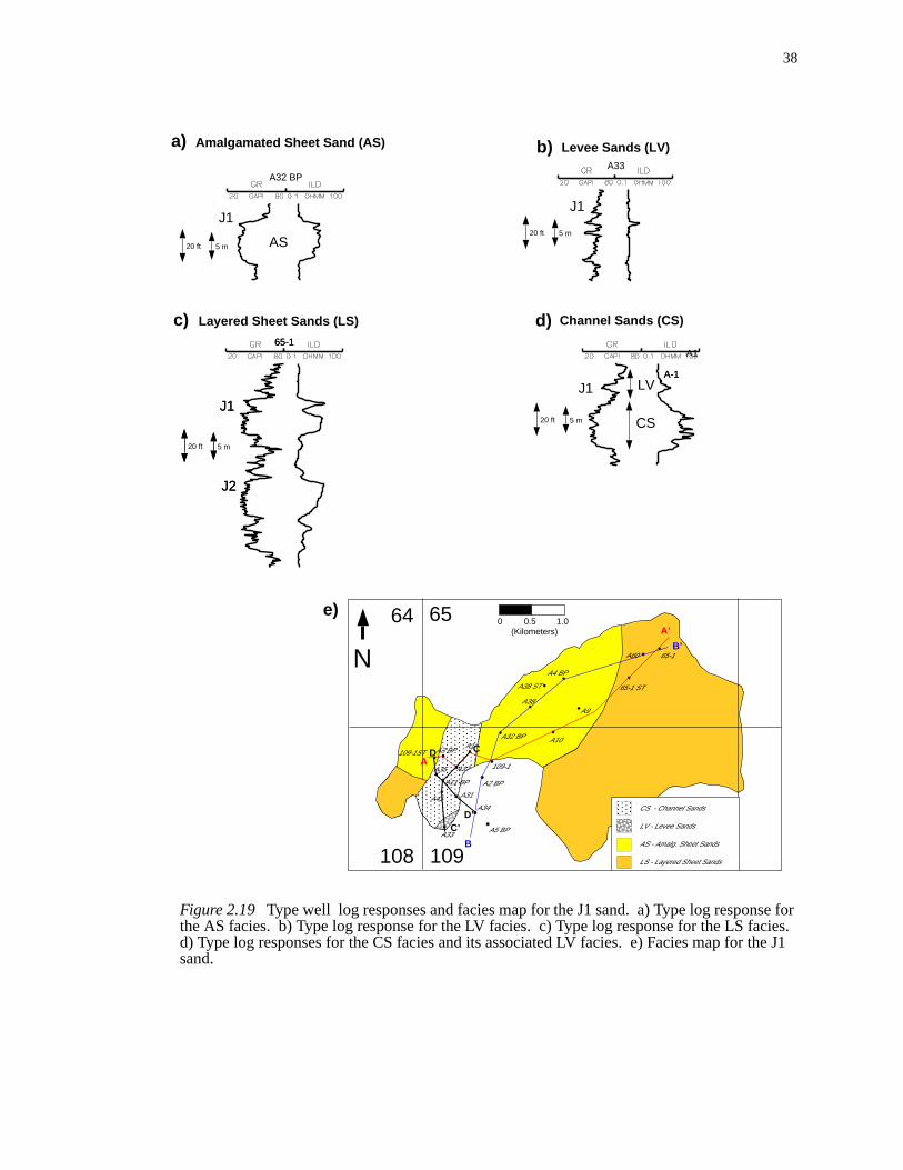
2.19 Type well log responses and facies map for the J1 sand(a) Type log response for the AS facies(b) Type well log response for the LV facies(c) Type log response for the LS facies(d) Type well log response for the CS facies(e) Facies map for the J1 sand

38

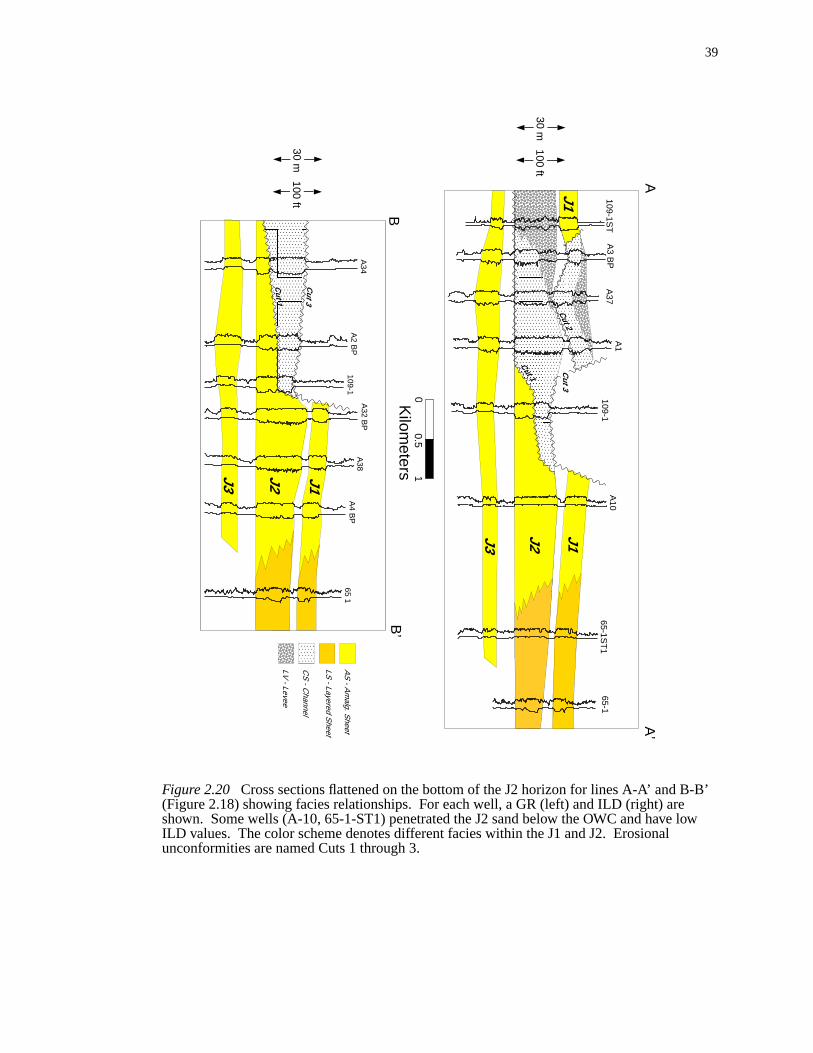
2.20 Cross sections flattened on the bottom of the J2 sand

2.21 Wireline responses of the CS and AS facies in the 109-1

2.22 Cross-sections through the J1 and J2 showing sand-on-sand contactsbetween the two reservoirs from the maps in Figures 2.18 and 2.19

46

2.23 Type well log responses for the flow units in the J2 sand(a) Type log for Unit 1(b) Flow unit map for the J2 sand(c) Type log for the Unit 2(d) Type logs for Unit 4(e) Type log for Unit 6

49

2.24 Type well log responses for the flow units in the J2 sand(a) Type log for Unit 1(b) Flow unit map for the J2 sand(c) Type log for the Unit 2(d) Type logs for Unit 4(e) Type log for Unit 6

50

viii

1

2

5

0

9

1

2.25 Wireline responses of the AS facies in the A32 BP 5

2.26 Wireline responses of the LS facies in the 65-1 5

2.27 Wireline responses of the LV facies in the 109-1-ST 5

3.1 J2 net pay in 1989 with seismic survey amplitudes 7

3.2 J1 net pay in 1989 71

3.3 Production data from the A32 BP 73

3.4 Date of initial water production, 50% water-cut, and shut-in for allwells producing from the J1 and J2

75

3.5 PNC log suite from the A32 BP 76

3.6 Floodout plot showing depths and times during which each well inthe J1 and J2 began showing water, either in the form of water pro-duction or from PNC log interpretation

77

3.7 Structural location of the OWC through time in the J2 7

3.8 Structural location of the OWC through time in the J1 8

3.9 Dip cross-section through the J1 and J2 sands illustrating verticalmovement of the OWC through time

84

3.10 Net pay map for the J2 in 1997 85

3.11 Net pay map for the J1 in 1997 86

3.12 Schematic illustrating the physical meaning of a net pay differencemap

88

3.13 Drained pay difference map for the J2 89

3.14 Drained pay difference map for the J1 90

3.15 Effective stress, porosity, and Vp observations from the J Sands(a) Porosity vs. effective stress(b) Vp vs. porosity(c) Vp vs. effective stress(d) Vp vs. porosity

96

ix

110

3.16 Relationships between Kdry, effective stress, and porosity for theBullwinkle J Sands

(a) Kdry vs. effective stress(b) Kdry vs. porosity

98

3.17 Kdry/effective stress model using laboratory data from Blangy (1992)(a) Kdry vs. effective stress(b) Kdry vs. effective stress paths

100

3.18 Vp/effective stress model(a) Vp vs. effective stress(b) Vp vs. effective stress paths

103

3.19 Expected changes in acoustic properties due to changes in Sw(a) Vp vs. Sw(b) Impedance vs. Sw(c) RFC vs. Sw

105

3.20 Acoustic property changes in the 109-1 J2 as a function of Sw andeffective stress

(a) Vp as a function of Sw and effective stress(b) Impedance as a function of Sw and effective stress(c) RFC as a function of Sw and effective stress

109

3.21 Gassmann fluid substitution logs for the J2 and J3 Sands in the 109-1

3.22 Seismic model for water-sweep in the 109-1 J2 Sand(a) Extracted traces from the 1988 survey and synthetic trace(b) Comparison of observed and modeled seismic differences

111

3.23 Acoustic property changes in the A33 as a function of Sw and effec-tive stress

(a) Vp as a function of Sw and effective stress(b) Impedance as a function of Sw and effective stress(c) RFC as a function of Sw and effective stress

114

3.24 Seismic model for gas exsolution in the A33(a) Extracted traces from the 1988 survey and synthetic trace(b) Comparison of observed and modeled seismic differences

116

x

1

3.25 Acoustic properties of the J2 as a function of depth at 1989 and 1997conditions

(a) Vp as a function depth(b) Impedance as a function depth(c) RFC as a function of depth

117

A.1 Openhole and PNC log analysis in the A-37 13

xi

1

3

5

3

125

25

3

4

List of Tables

2.1 Average petrophysical properties for each well 6

2.2 Whole core data from the A32 BP and 65-1 ST1 wells used in the anal-ysis of electrical resistivity data.

62

2.3 Drainage and imbibition data from the A32 BP and 65-1 ST1 wholecores

63

2.4 Resisitivity Data from A32 BP and 65-1 ST1 whole cores 6

2.5 Whole core porosity and permeability measured under 2100 psi effec-tive stress from the A32 BP well. Vsh was taken from GR log.

64

2.6 Average petrophysical properties for each flow unit 6

3.1 Reservoir Volumes for the J1 and J2 RB reservoirs at initial (1989) andpost-production (1997) conditions.

122

3.2 Production data summary for the J1 and J2 RB 12

3.3 Summary of sonic and porosity log data taken from the water leg of theJ1, J2 and J3 sands

124

3.4 Fluid properties used for investigating the influence on hydrocarbon sat-uration on the acoustic properties of the 109-1 J2 sand.

124

3.5 Elastic properties of the 109-1 J2 used in Gassmann modeling

3.6 Acoustic properties of the A33 used in Gassmann modeling 1

B.1 Parameters used for 1989 Conditions 13

B.2 Parameters used for 1997 Conditions 13

xii

spon-

,

ime-

Shell

oft-

hysi-

ny-

d to

o Tur-

Geo-

y fel-

ork

any

and

ther

s of

ir

Acknowledgements

This research is part of the Penn State Petroleum Geosystems Initiative, which is

sored by Shell Exploration and Production Company (SEPCo), the Shell Foundation

IBM, and Landmark Graphics. Additional support was provided by the Penn State T

Lapse Consortium, whose members include Chevron, Conoco, Statoil, and Texaco.

were very helpful in providing and releasing much of the data used in this project. S

ware support was supplied by Landmark Graphics Corporation and Paradigm Geop

cal.

I would first like to thank my advisor, Peter Flemings, for introducing me to the ma

faceted problems in petroleum geology and how they are solved. I am also indebte

my thesis committee members, Phil Halleck and Chris Marone. Thanks also goes t

gay Ertekin and Terry Engelder for their additional input and advice to the Petroleum

systems Initiative.

My research would not have been possible without the input and hard work of m

low Geosystems teammates, Alastair Swanston and Kevin Best. Much of Alastair’s w

lays the foundation for the time-lapse analysis of Chapter 3. Kevin and I have spent m

hours discussing and working through the reservoir engineering aspects of Bullwinkle

his insight, hard work, and diligence has been invaluable. Rachel Altemus and Hea

Johnson keep everything running and organized and have always been there in time

need. Additional thanks goes to Brandon Dugan, Jacek Lupa, and Xiaoli Liu for the

insights into compaction and fluid flow.

xiii

r-

to

at

Bill

nal-

e

ll of

The geoscientists at Shell who have helped the team along our two year journey

include Dave Miller, Mahdu Kholi, Tucker Burkhart, A.J. Durani, Tom Wilson, Mike Ba

onovic and Mike Kuzio.

Additional thanks go to the Formation Evaluation group at the Chevron Petroleum

Technology Company in San Ramon, CA. Bill Corea and Barry Reik introduced me

some of the more complicated aspects of well log analysis and made my internship

Chevron very rewarding. I would also like to thank Bruce Bilodeau, Simon Stonard,

Ballengee, and Rick Abegg at Chevron for all of their advice on careers and well log a

ysis.

Finally, I would like to thank my family and friends for all of their support and positiv

karma. My parents have been an instrumental part of my life and I thank them for a

their help.

1

Bull-

J

core

and I

ati-

d to

abil-

amic

cost

e at

high

reser-

ing

na-

ull-

ysis

and

ater-

eep

Chapter 1

INTRODUCTION

This thesis addresses both the static and dynamic behavior of the J Sands in the

winkle Field. Chapter 2 begins at the grain scale, where the initial conditions of the

Sands are characterized in terms of porosity, permeability, and water saturation using

and well log data. A depositional model for the turbiditic J Sands is then presented

show that rock properties in the field are spatially controlled by the distribution of str

graphic facies. The rock property observations and depositional model are then use

create the initial reservoir simulation model which incorporates the stratigraphic vari

ity inherent in deepwater turbidite reservoir systems. Chapter 3 characterizes the dyn

behavior of the Bullwinkle J Sands observed at the well and seismic scale. The high

of exploring and producing in the deepwater Gulf of Mexico requires that wells produc

rates greater than 5000 barrels of oil per day to be profitable (Lawrence, 1994). Such

sustained flow rates are achieved more frequently when the knowledge base of the

voir system is optimized over this wide variety of spatial and temporal scales.

The importance of relating different types of data at a variety of scales is a recurr

theme throughout this thesis. We relate core-measured properties to the well log sig

tures and then use these well log signatures to devise a depositional model for the B

winkle J Sands. Production data, cased hole well logs, and time-lapse seismic anal

provide us with tools which we used to characterize the dynamic behavior of the J S

reservoirs. Rock physics modeling aided in interpreting the time-lapse signature of w

sweep and gas exsolution. The rock physics model predicted that areas of water sw

2

water

in the

93)

d in

tional

er-

fields

nts

in

ron-

pes

h

ier

func-

er-

ty in

t the

how

fset)

experienced a dramatic decrease in seismic amplitude through time. These areas of

sweep were also verified by the production data and cased hole log analysis.

Characterization of deepwater turbidites has been the focus of many field studies

Gulf of Mexico (Holman and Robertson, 1994; Mahaffie, 1994). O’Connell et al. (19

addressed the importance of seismic survey design and acquisition parameters use

imaging the Bullwinkle J Sands. Holman and Robertson (1994) presented a deposi

model for the Bullwinkle J Sands and showed how their interpretation of turbidite res

voir connectivity and architecture fit into the slope mini-basin model of Prather et al.

(1998). McGee et al. (1994) and Kendrick (2000) characterized several deepwater

and show how the spatial and temporal changes in turbidite depositional environme

effect the production strategies used in each case. A similar study for the K40 sand

South Timbalier Block 295 demonstrated how subsurface turbidite depositional envi

ments can be compared with outcrop analogs (Hoover, 1997).

Rock properties for deepwater Gulf of Mexico turbidites are favorable for these ty

of integrated reservoir studies. In general, they consist of unconsolidated sands wit

extremely high porosity (0.28 to 0.34) and permeability (100 to 3000 mD). Osterme

(1995) studied the changes in porosity and permeability for these types of sands as a

tion of compressibility and effective stress. He found that highly porous turbidite res

voirs have extremely high compressibilities and that reduction in porosity due to

compaction drastically reduces permeability. Flemings et al. (2001) show that porosi

the J3 sand at Bullwinkle is stress controlled, in that higher porosity sands are found a

top of structure where the effective stress is lower. Blangy (1992) and Clark (1992) s

that direct hydrocarbon indicators such as bright spots and AVO (amplitude versus of

3

cous-

ears

es of

me.

on

n and

mi-

ter

l log

dy of

w)

ys.

n sim-

l out-

ain-

are a result of highly porous unconsolidated hydrocarbon sands having much lower a

tic impedances than the shales which bound them.

The dynamic behavior of reservoirs has been studied extensively in the past few y

in the form of time-lapse (4D) studies. Hoover et al., (1999) performed an integrated

time-lapse analysis for the K40 channel turbidite reservoir and demonstrated that zon

water-sweep were associated with strong decrease in seismic amplitudes through ti

Hoover et al. (1999) also tracked oil-water contact (OWC) movement using producti

and log data. Packwood (1997) used a rock physics model which combined saturatio

pressure changes to show how coning of gas during primary oil production was seis

cally visible for very high porosity rocks. Landro et al. (1999) demonstrated how wa

movement predicted on the basis of time-lapse seismic data were confirmed by wel

and production data observations. Behrens et al.(2001) performed a time-lapse stu

the Bay Marchand field in the Gulf of Mexico field and found that amplitude changes

through time were consistent with production data and rock physics models.

This thesis is part of a larger study of the Bullwinkle field. Swanston et al. (in revie

present a detailed time-lapse study of the Bullwinkle field using multiple seismic surve

They show that time-lapse analysis provides the best results when two surveys shot i

ilar directions are normalized and differenced. Best (2002) used the geologic mode

lined in this thesis as an input for the J1/J2 reservoir simulation. He found that

compaction-induced water influx and sand connectivity has played a major role in m

taining pressures in the reservoir during production.

4

ser-65,

in

ndan-

is ofpse

Tim-smic

lds,Char-

ks

o, Tur-

ery,

ogic

Tur-

References

Best, K.D., 2002, Development of an integrated model for compaction/water drive revoirs and its application to the J1 and J2 Sand at Bullwinkle, Green Canyon BlockGulf of Mexico: Masters thesis, The Pennsylvania State University.

Flemings, P.B., Comisky, J., Liu, X., and Lupa, J.A., 2001, Stress-controlled porosityoverpressured sands at Bullwinkle (GC65), Deepwater GoM.Offshore TechnologyConference, April 30- May 3, 2001.

Holman, W.E., and Robertson, S.S., 1994, Field development, depositional model, aproduction performance of the turbiditic “J” Sands at Prospect Bullwinkle, Green Cyon 65 Field, outer-shelf Gulf of Mexico,GCSSEPM Foundation 15th AnnualResearch Conference, Submarine Fans and Turbidite Systems, December 4-7, p. 139-150.

Hoover, A.R., Burkhart, T.B., Flemings, P.B., 1999, Reservoir and production analysthe K40 sand, South Timbalier 295, offshore Louisiana, with comparison to time-la(4-D) seismic results.AAPG Bulletin, v. 83, no. 10, pp. 1624-1641.

Hoover, A.R., 1997, Reservoir and production characteristics of the K40 sand, Southbalier 295, offshore Louisiana with outcrop analogues and comparison to 4D seiresults: Masters thesis, The Pennsylvania State University.

Kendrick, J.W., 2000, Turbidite reservoir architecture in the northern Gulf of Mexicodeepwater: insights from the development of Auger, Tahoe, and Ram/Powell FieGCSSEPM Foundation 20th Annual Research Conference Advanced Reservoir acterization, December 5-8, pp. 450-468.

Landro, M., Solheim, O.A., Hilde, E., Ekren, B.O., and Stronen, L.K., 1999, The Gulfa4D seismic study: Petroleum Geoscience, vol 5, pp. 213 - 226.

Lawrence, D.T., 1994, Turbidite technical challenges in the deepwater Gulf of MexicGCSSEPM Foundation 15th Annual Research Conference, Submarine Fans andbidite Systems, December 4-7, pp. 217-219.

Mahaffie, M.J., 1994, Reservoir classification for turbidite intervals at the Mars discovMississippi Canyon 807, Gulf of Mexico.GCSSEPM Foundation 15th AnnualResearch Conference, Submarine Fans and Turbidite Systems,December 4-7, p. 233-244.

McGee, D.T., Bilinski, P.B., Gary, P.S., Pfeiffer, D.S., and Sheiman. J.L., 1994, Geolmodels and reservoir geometries of Auger field, deepwater Gulf of Mexico,GCSSEPM Foundation 15th Annual Research Conference, Submarine Fans andbidite Systems, December 4-7, p. 245-256.

5

ros-

g

Ostermeier, R.M., 1995, Deepwater Gulf of Mexico turbidite compaction effects on poity and permeability.SPE Formation Evaluation, v. 10, No. 2, pp. 79-85.

Packwood, J.L., 1996, Feasibility of hydrocarbon recovery monitoring with increasinrock frame stiffness: SEG Expanded Abstract, pp. 876 - 878.

6

mbi-

all into

ive

alysis

d the

each

ble

spec-

tivity

e chan-

n

pths

as

Chapter 2

FORMATION EVALUATION AND DEPOSITIONAL MODEL FORTHE BULLWINKLE J SANDS, GREEN CANYON BLOCK 65, OFF-

SHORE LOUISIANA

Abstract

The J1 and J2 reservoirs of the Bullwinkle field in Green Canyon 65 contain a co

nation of interconnected sheet and channel sand facies. The J1 and J2 reservoirs f

the slope turbidite model of Prather et al. (1998) where deposition of laterally extens

sheet sands was followed by periods of channel cutting and deposition. Well log an

shows that rock properties are facies dependent and vary across the field. We use

depositional model to break out the facies of the J1 and J2 into separate flow units,

with its own rock properties. The thick, clean sheet sand facies has the most favora

rock properties, with an average porosity and permeability of 0.33 and 2400 mD, re

tively. The depositional model also sheds some insight into the nature of the connec

between the J1 and J2 reservoirs. The J1 and J2 hydraulically communicate becaus

nel facies have cut through the shale separating both reservoirs.

Introduction

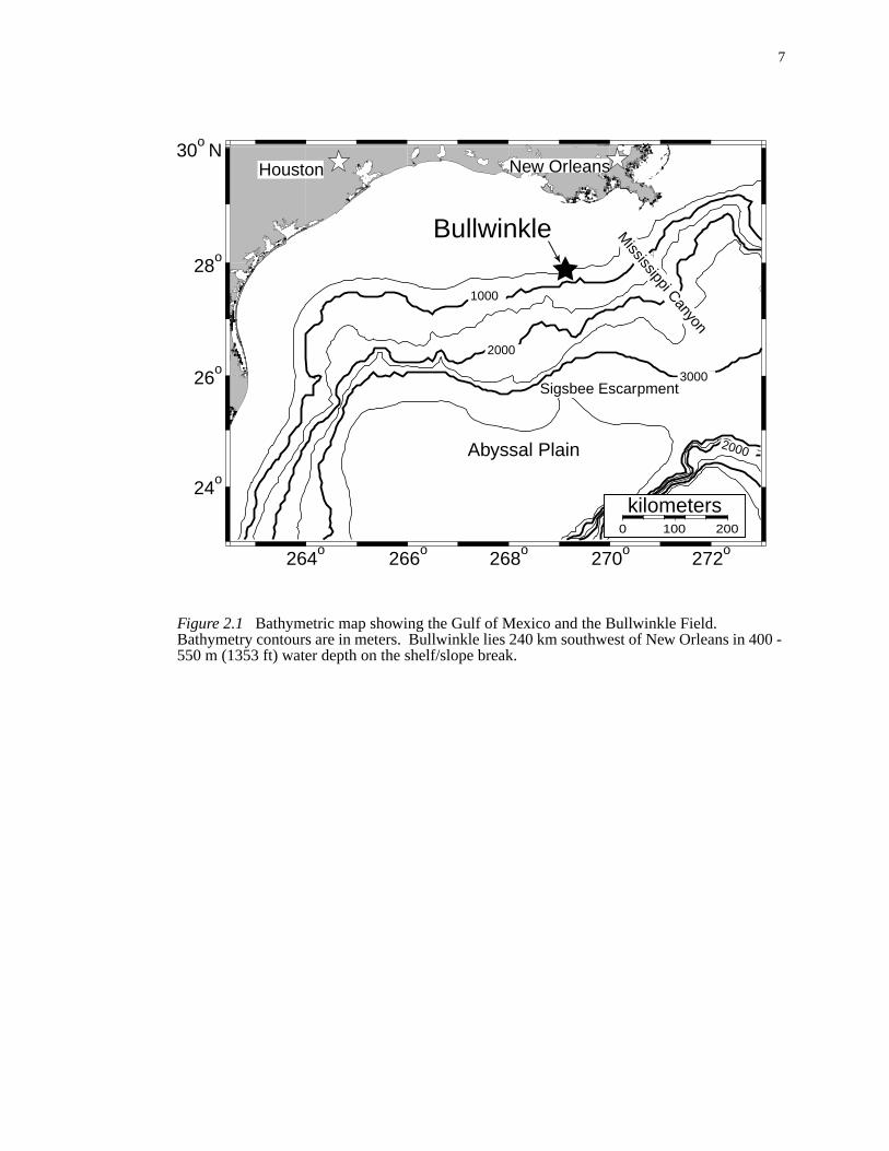
The Bullwinkle field is located 240 km southwest of New Orleans in Green Canyo

Blocks 64, 65, and 109 (Figure 2.1). It is located on the slope-shelf break, in water de

ranging from 400 to 550 m (O’Connell et al., 1993). The initial discovery well (65-1) w

7

00 -
Figure 2.1 Bathymetric map showing the Gulf of Mexico and the Bullwinkle Field.Bathymetry contours are in meters. Bullwinkle lies 240 km southwest of New Orleans in 4550 m (1353 ft) water depth on the shelf/slope break.
-2000

0

0

Abyssal Plain

264o

24o

26o

28o

30o N

266o 268o 270o 272o

Houston New Orleans

Mississippi Canyon

Sigsbee Escarpment

Bullwinkle

0 100 200

kilometers

3000

2000

1000

2000

8

d the

r the

ra-

9

r res-

ves

an-

ce

J1

-oil

n-

a

u-

tural

m

e J2

re

he

drilled in 1983 and it penetrated the J1 and J2 sands. O’Connell et al. (1993) describe

acquisition and interpretation of two orthogonal 3-D seismic surveys shot in 1988 fo

Bullwinkle field which were used for initial development mapping. Several other explo

tion wells (109-1, 109-1ST, 65-1-ST) were drilled and initial production began in 198

from the Bullwinkle platform. Production from the J Sands and several other smalle

ervoirs have produced over 130 MMBOE (million barrels of oil equivalent) with reser

estimated at 160 MMBOE (Holman and Robertson, 1994).

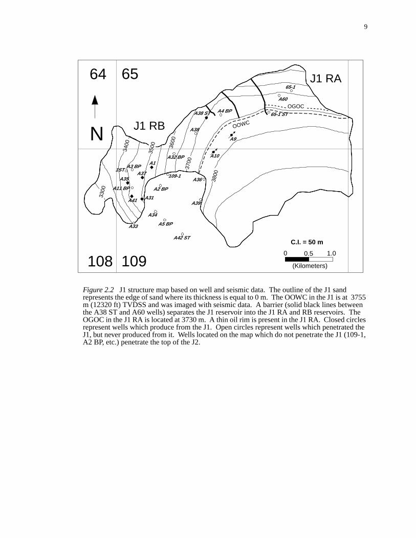
The J1 reservoir is located on the western flank of the basin, primarily in Green C

yon Blocks 109 and 65 (Figure 2.2). It has approximately 600 m (2000 ft) of vertical

relief with an original oil-water contact (OOWC) located at 3755 m (12230 ft) subsurfa

total vertical depth (TVDSS). A flow barrier separates the J1 into two reservoirs, the

RA and J1 RB, each with its own type of hydrocarbon fluids. The J1 RA original gas

contact (OGOC) is located at 3730 m. The presence of a gas cap in the J1 RA is co

firmed by well logs in the 65-1 and fluid samples. The J1 RB initially did not contain

gas cap. Well and production data in the J1 RB confirm that it was initially undersat

rated.

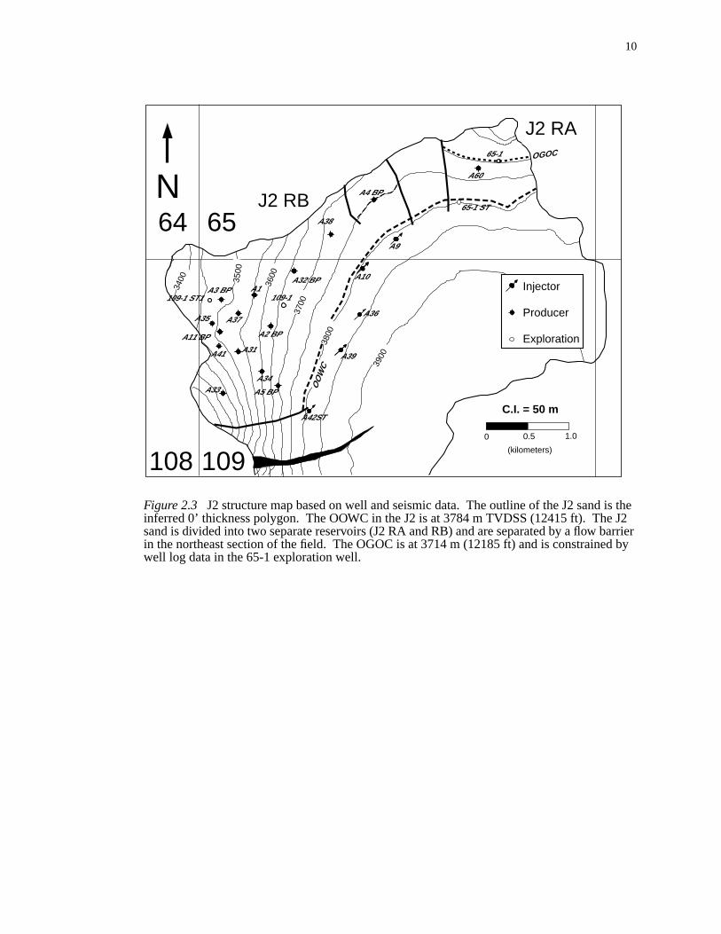
The J2 sand is volumetrically larger than the J1, but shows many of the same struc

characteristics (Figure 2.3). Seismic data and well control place the OOWC at 3784

(12415 ft). The J2 is also divided into two separate reservoirs (J2 RA and J2 RB). Th

RB is initially undersaturated and is separated from the J2 RA by a flow barrier (Figu

2.3). The J2 RA is a gas cap reservoir, with an OGOC located at 3714 m (3713). T

9

3755een Theles

ed the09-1,

Figure 2.2 J1 structure map based on well and seismic data. The outline of the J1 sandrepresents the edge of sand where its thickness is equal to 0 m. The OOWC in the J1 is atm (12320 ft) TVDSS and was imaged with seismic data. A barrier (solid black lines betwthe A38 ST and A60 wells) separates the J1 reservoir into the J1 RA and RB reservoirs. OGOC in the J1 RA is located at 3730 m. A thin oil rim is present in the J1 RA. Closed circrepresent wells which produce from the J1. Open circles represent wells which penetratJ1, but never produced from it. Wells located on the map which do not penetrate the J1 (1A2 BP, etc.) penetrate the top of the J2.

A31

A33

A32 BP

A38

A38 ST A4 BP65-1 ST

A60

65-1

A35

A3 BPA1

A41

A37

65

109108

64

0 0.5 1.0

(Kilometers)

N

A5 BP

109-1

A2 BP

C.I. = 50 m

A34

A11 BP

1ST

A42 ST

A39

A36

A10

A9

3500 36

00

3700

3800

3400

3300

OOWC

OGOC

J1 RA

J1 RB

10

is the J2arrierd by

Figure 2.3 J2 structure map based on well and seismic data. The outline of the J2 sandinferred 0’ thickness polygon. The OOWC in the J2 is at 3784 m TVDSS (12415 ft). Thesand is divided into two separate reservoirs (J2 RA and RB) and are separated by a flow bin the northeast section of the field. The OGOC is at 3714 m (12185 ft) and is constrainewell log data in the 65-1 exploration well.

N

109-1 ST1A1

A35

A11 BP

A41

A33A34

A37

A5 BP

A36

A3 BP109-1

A32 BP

A2 BP

A38

A10

A4 BP

65-1 ST

A60

65-1

A9

Injector

Producer

Exploration

0 0.5 1.0

(kilometers)

A42ST

A39A31

65

109108

64

C.I. = 50 m

3900

3800

3700

36003500

3400

OOWC

OGOC

J2 RA

J2 RB

11

in

han-

hitec-

re

). The

cribed

ell

ture,

facies

are

the

ort and

ulk

OGOC in the J2 RA was imaged with porosity logs in the initial exploration well (65-1

Figure 2.3).

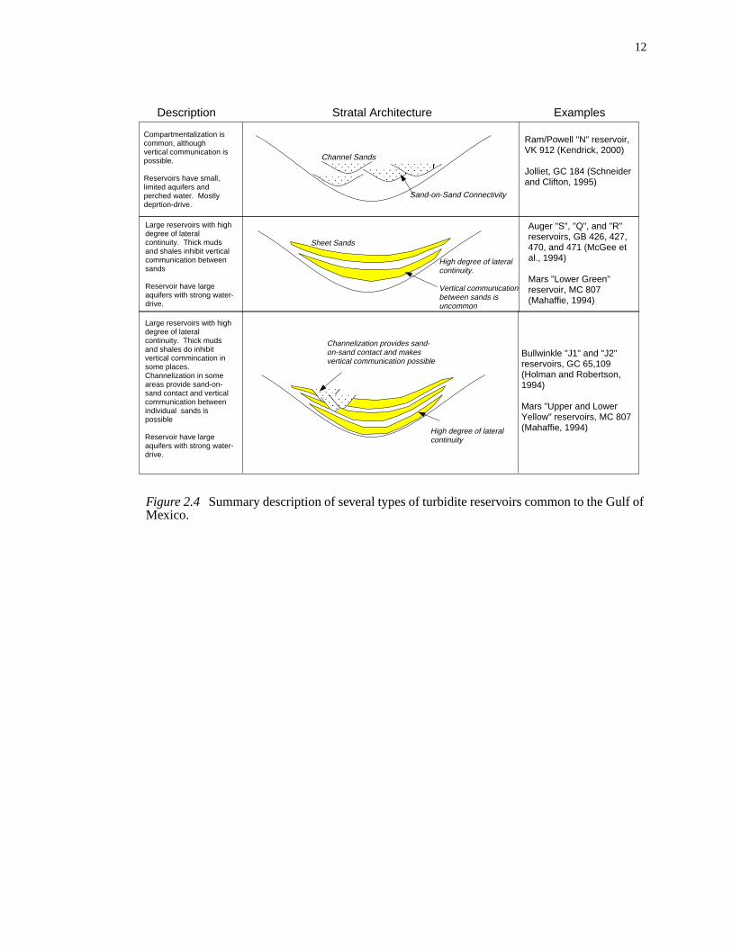
The Bullwinkle J1 and J2 sands are composed of both amalgamated sheet and c

nelized turbidite sands. Sheet sands within the J1 and J2 follow the same type of arc

ture as the Auger Field described by McGee et al. (1994) and Kendrick (2000), whe

continuous sheet sands are vertically separated by thick muds and shales (Figure 2.4

log character of the channelized sands in the J1 and J2 are similar to the sands des

by Kendrick (2000) for the Ram-Powell field. However, the reservoirs within Ram-Pow

are highly compartmentalized due to the channelized nature of the reservoir architec

where perched water contacts and depletion style reservoirs are common.

The J1 and J2 sands are both strong water-drive reservoirs due to the sheet sand

which extend throughout the Bullwinkle basin. Some sheet sand individual reservoirs

not in hydraulic communication due to the thick layers of shale separating them. In

case of the J1 and J2, however, laterally extensive sheet sands provide water supp

the channel facies provide sand-on-sand contacts making hydraulic communication

between both reservoirs possible (Figure 2.4).

Formation Evaluation

Porosity

Log-based porosity calculations for the Bullwinkle J Sands were taken from the b

density log where

. (2.1)φρg ρb–

ρg ρ f–-----------------=

12

lf of
Figure 2.4 Summary description of several types of turbidite reservoirs common to the GuMexico.
Channel Sands

Sand-on-Sand Connectivity

Compartmentalization is common, although vertical communication is possible.

Reservoirs have small, limited aquifers and perched water. Mostly deprtion-drive.

Large reservoirs with high degree of lateral continuity. Thick muds and shales inhibit vertical communication between sands

Reservoir have large aquifers with strong water-drive.

Sheet Sands

High degree of lateralcontinuity.

Vertical communication between sands is uncommon

High degree of lateralcontinuity

Channelization provides sand-on-sand contact and makesvertical communication possible

Large reservoirs with high degree of lateral continuity. Thick muds and shales do inhibit vertical commincation in some places. Channelization in some areas provide sand-on-sand contact and vertical communication between individual sands is possible

Reservoir have large aquifers with strong water-drive.

Description Stratal Architecture Examples

Auger "S", "Q", and "R" reservoirs, GB 426, 427, 470, and 471 (McGee et al., 1994)

Mars "Lower Green" reservoir, MC 807 (Mahaffie, 1994)

Ram/Powell "N" reservoir,VK 912 (Kendrick, 2000)

Jolliet, GC 184 (Schneider and Clifton, 1995)

Bullwinkle "J1" and "J2" reservoirs, GC 65,109(Holman and Robertson,1994)

Mars "Upper and Lower Yellow" reservoirs, MC 807(Mahaffie, 1994)

13

as

tool

sity

2.5).

ree-

uid

te

. A

(Bat-

.u.)

en a

re oil

e 2.7)

cc

fluid

0.98

ons

ed in

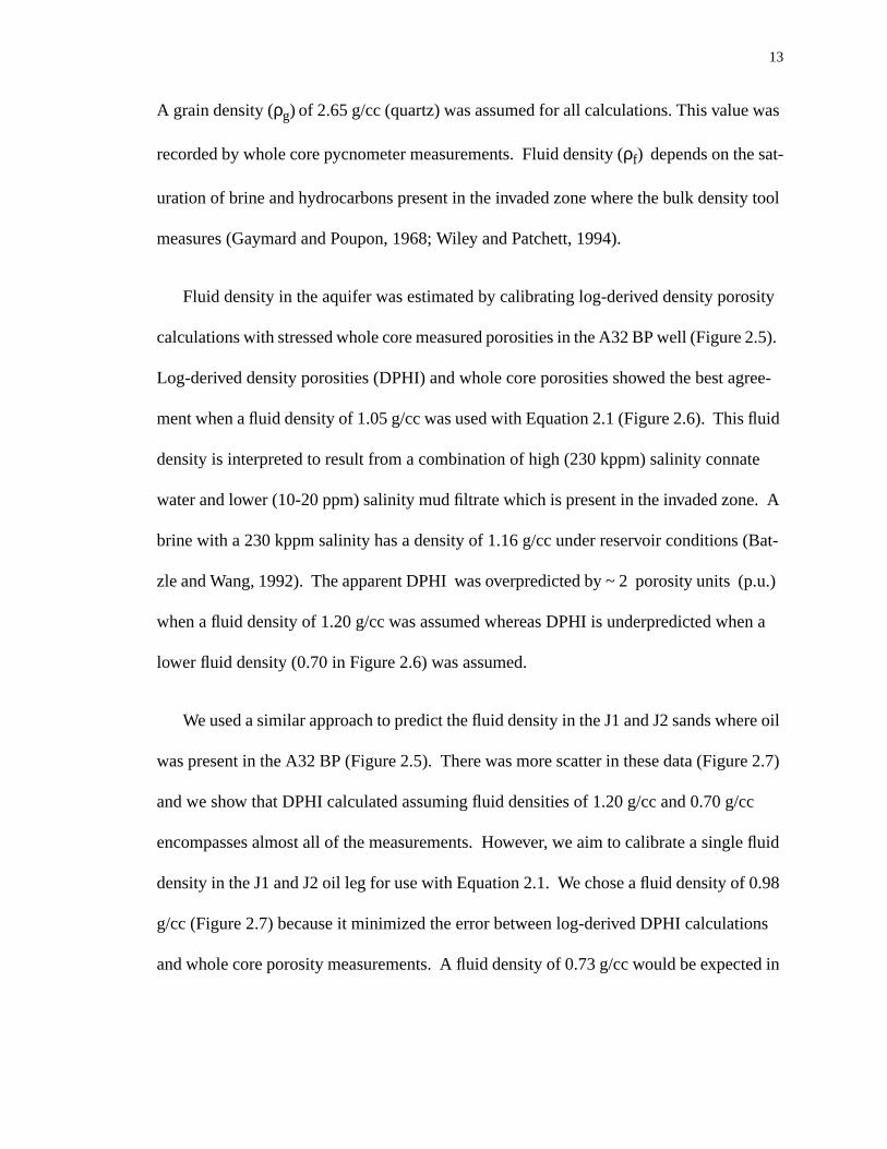
A grain density (ρg) of 2.65 g/cc (quartz) was assumed for all calculations. This value w

recorded by whole core pycnometer measurements. Fluid density (ρf) depends on the sat-

uration of brine and hydrocarbons present in the invaded zone where the bulk density

measures (Gaymard and Poupon, 1968; Wiley and Patchett, 1994).

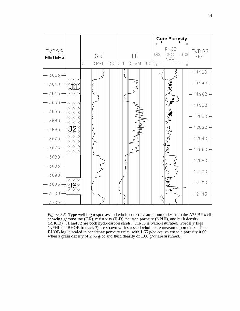
Fluid density in the aquifer was estimated by calibrating log-derived density poro

calculations with stressed whole core measured porosities in the A32 BP well (Figure

Log-derived density porosities (DPHI) and whole core porosities showed the best ag

ment when a fluid density of 1.05 g/cc was used with Equation 2.1 (Figure 2.6). This fl

density is interpreted to result from a combination of high (230 kppm) salinity conna

water and lower (10-20 ppm) salinity mud filtrate which is present in the invaded zone

brine with a 230 kppm salinity has a density of 1.16 g/cc under reservoir conditions

zle and Wang, 1992). The apparent DPHI was overpredicted by ~ 2 porosity units (p

when a fluid density of 1.20 g/cc was assumed whereas DPHI is underpredicted wh

lower fluid density (0.70 in Figure 2.6) was assumed.

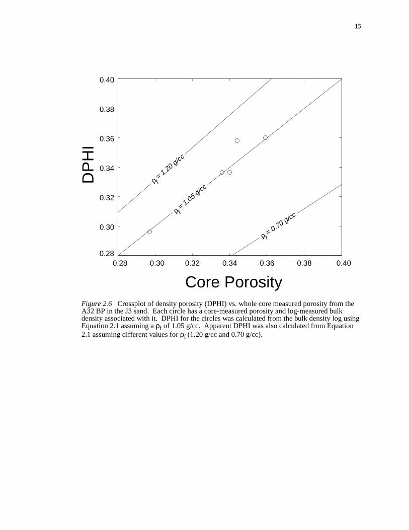
We used a similar approach to predict the fluid density in the J1 and J2 sands whe

was present in the A32 BP (Figure 2.5). There was more scatter in these data (Figur

and we show that DPHI calculated assuming fluid densities of 1.20 g/cc and 0.70 g/

encompasses almost all of the measurements. However, we aim to calibrate a single

density in the J1 and J2 oil leg for use with Equation 2.1. We chose a fluid density of

g/cc (Figure 2.7) because it minimized the error between log-derived DPHI calculati

and whole core porosity measurements. A fluid density of 0.73 g/cc would be expect

14

well

gshe60

Figure 2.5 Type well log responses and whole core-measured porosities from the A32 BPshowing gamma-ray (GR), resistivity (ILD), neutron porosity (NPHI), and bulk density(RHOB). J1 and J2 are both hydrocarbon sands. The J3 is water-saturated. Porosity lo(NPHI and RHOB in track 3) are shown with stressed whole core measured porosities. TRHOB log is scaled in sandstone porosity units, with 1.65 g/cc equivalent to a porosity 0.when a grain density of 2.65 g/cc and fluid density of 1.00 g/cc are assumed.

J3

J2

J1

METERS

Core Porosity

15

eksing

Figure 2.6 Crossplot of density porosity (DPHI) vs. whole core measured porosity from thA32 BP in the J3 sand. Each circle has a core-measured porosity and log-measured buldensity associated with it. DPHI for the circles was calculated from the bulk density log uEquation 2.1 assuming aρf of 1.05 g/cc. Apparent DPHI was also calculated from Equation2.1 assuming different values forρf (1.20 g/cc and 0.70 g/cc).

0.30 0.32 0.34 0.36 0.38 0.40

0.30

0.32

0.34

0.36

0.38

0.40

DP

HI

Core Porosity

ρ = 1.20 g/cc

f

ρ = 1.05 g/cc

f

ρ = 0.70 g/cc

f

0.280.28

16

coreanhow a

Figure 2.7 Crossplot of log-predicted density porosity (DPHI) vs. stressed whole coreporosities in the J1 and J2 sands from the A32 BP well (Figure 2.5). a) DPHI and wholeporosities have the best agreement when aρf of 0.98 g/cc is used with Equation 2.1. The datshow a very wide range of possibleρf (1.20 g/cc to 0.70 g/cc). b) Enlargement of boxed regioin Figure 2.7a. The core data are broken into J1 and J2 samples. Data from both sands sscatter about the 1:1 correlation line, corresponding to aρf of 0.98 g/cc.

0

0.10

0.20

0.30

0.40

0.50

0.60

0.70

0.80

0.90

1.00

DP

HI

Core Porosity

DP

HI

0.22 0.26 0.30 0.34 0.38

0.22

0.26

0.30

0.34

0.38 J1J2

Core Porosity

ρ = 1.20 g/cc

f

ρ = 0.98 g/cc

f

ρ = 0.70 g/cc

f

0.36

0.32

0.28

0.24

0.20

0.40

0 0.10 0.20 0.30 0.40 0.50 0.60 0.70 0.80 0.90 1.00

ρ = 1.20 g/cc

f

ρ = 0.98 g/cc

f

ρ = 0.70 g/cc

f

0.20 0.24 0.28 0.32 0.36 0.40

a)

b)

17

0.65

uid

l leg

to

i-

ma-

ume

g/cc.

ng

its vir-

ewall

bulk

roce-

he J1

re

ints

o-one

rify

the uninvaded zone of the oil-filled J Sands assuming typical values for oil density (

g/cc), connate water density (1.16 g/cc) and water saturation (0.15). However, the fl

density we calibrated using whole core and bulk density log measurements in the oi

(0.98 g/cc) is considerably higher than 0.73 g/cc. We infer that this difference is due

invasion of mud filtrate into the formation during drilling. The bulk density tool invest

gates the invaded zone of the formation, where mud filtrate flushes out the virgin for

tion fluids and leaves behind irreducible water and residual hydrocarbons. If we ass

that irreducible water (Sw = 0.15), mud filtrate (pmf = 1.05 g/cc), and residual oil (Sor =

0.25) are present in the invaded zone, we would expect a fluid density closer to 0.97

This value for fluid density in the oil leg is much closer to the value we calibrated usi

DPHI and core measurements and suggests that the formation has been flushed of

gin fluids during the drilling process.

Fluid density in the gas cap of the J1 and J2 reservoirs was constrained using sid

core data from the 65-1 well. The J1 in the 65-1 is interpreted as a gas zone due to

density/neutron porosity (RHOB/NPHI) crossover (Figure 2.8). We used the same p

dure presented in Figures 2.6 and 2.7 to predict the fluid density in the gas zone of t

and J2. A fluid density of 0.68 g/cc most closely matched the DPHI and sidewall co

porosities for the 65-1 in the gas zones (Figure 2.9). A fluid density of 0.98 g/cc was

assumed for calculating DPHI in the oil leg of the J2 from the 65-1. The oil leg data po

show the same type of scatter as in Figure 2.7 , but are distributed around the one-t

correlation line in Figure 2.9 . The oil leg data points in Figure 2.9 independently ve

the fluid density of 0.98 g/cc we calibrated in the A32 BP.

18

ones.
Figure 2.8 Well log responses from the 65-1 well which penetrated the J1 and J2 sands(Figures 2.2 and 2.3). Apparent RHOB/NPHI crossover in the J1 and J2 represent gas zSidewall core measurements of porosity show that NPHI is underpredicted and DPHI isoverpredicted in the gas zones assuming aρf of 1.00 g/cc for DPHI. The original gas-oilcontact (OGOC) was imaged in the J2 at 3714 m (12185 ft).
Sidewall Por

METERS

J1

J2 OGOC

}

Gas Effect

}}

RHOB1.65 2.65G/C3

19

me-

lem.

found

appro-

leg

e

PHI

en

HI/

, we

ed

ch

erage

eabil-

Castle and Byrnes (1998) used this approach to predict porosities in the low per

ability Medina Sandstone of Northwestern Pennsylvania where gas invasion is a prob

Avseth (2000) documented the effects of invasion on North Sea turbidite sands and

the best approach was to use core and bulk density measurements to back calculate

priate fluid densities.

An approach used in Flemings et al. (2001) which predicted fluid density in the oil

of the J3 without the use of core data was applied to the J1 and J2 and agree with thρf

calibration of 0.98 g/cc in Figure 2.7. In their approach, a trend between NPHI and D

was established in the water leg of the J3 using a fluid density of 1.05 g/cc. They th

found that a fluid density of 0.94 g/cc in the oil leg of the J3 reproduced the same NP

DPHI trend as seen in the water leg. When that same method was applied to the J2

found that a fluid density of 0.98 g/cc in the oil leg matched the NPHI/DPHI trend deriv

in the water leg.

Average values of porosity calculated from the bulk density log were taken at ea

penetration of the J1 and J2 in reservoir zones and are shown in Table 2.1 . The av

porosity was taken for each well in the clean sand zones where the log-derived perm

ity was greater than 10 mD. Equation 2.1 was solved assuming aρg of 2.65 g/cc for all

wells. A ρf of 0.98 was used in the oil legs of the J1 and J2 and aρf of 1.05 g/cc was used

in the water legs. Aρf of 0.68 g/cc was used in the gas zones of the 65-1.

20

sa

Figure 2.9 65-1 sidewall core porosities in oil and gas zones. DPHI in the gas zones wacalculated using Equation 2.1 using aρf of 0.68 g/cc. DPHI in oil zones was calculated usingρf of 0.98 g/cc.

0.24 0.28 0.32 0.36

0.24

0.28

0.32

0.36Gas (0.68 g/cc)

Oil (0.98 g/cc)D

PH

I

Core Porosity

21

fec-

s that

ro-

53;

mula

tones.

prac-

in et

qua-

er,

Water Saturation

Archie’s equations (Archie, 1942) were used to calculate water saturation (Sw) at each

well with porosity and resistivity logs. The underlying assumption when applying

Archie’s Law is that electrical conduction takes place through brine trapped in the ef

tive porosity (Edmundson, 1988). This assumption limits this approach to clean sand

do not contain electrically conducting clays.

Archie (1942) proposed that the resistivity of a brine-saturated rock (Ro) is propor-

tional to the resistivity of the brine in the pores (Rw ):

, (2.2)

where the formation factor (F) was empirically constrained. The formation factor is p

portional to the porosity (Archie, 1942; Winsauer et. al., 1952; Wyllie and Gregory, 19

Carothers, 1968):

, (2.3)

where a and m are both empirical constants. Equation 2.3 is called the Humble for

and Winsauer et al. (1952) suggested a = 0.62 and m = 2.15 for a majority of sands

The Humble formula has become widely used in the industry and is routinely put to

tice in cases where there are no core data available for empirical calibrations (Dvork

al., 1999).

The formation factor can be directly calculated when only brine is present using E

tion 2.2. In this approach, the deep resistivity log (ILD) is assumed to record Ro and the

brine resistivity (Rw) is interpreted from standard log interpretation charts (Schlumberg

Ro FRw=

Fa

φm------=

22

late F

nd

ents

s,

was

e

or by

ls

-

al.,

1989) given a salinity and temperature. For the Bullwinkle J Sands, Rw has an average

value of 0.022 ohm-m with brine salinity ranging from 210 to 230 kppm at 160o F. The

A36 well penetrated the J2 sand in the water leg (Figure 2.3) and was used to calcu

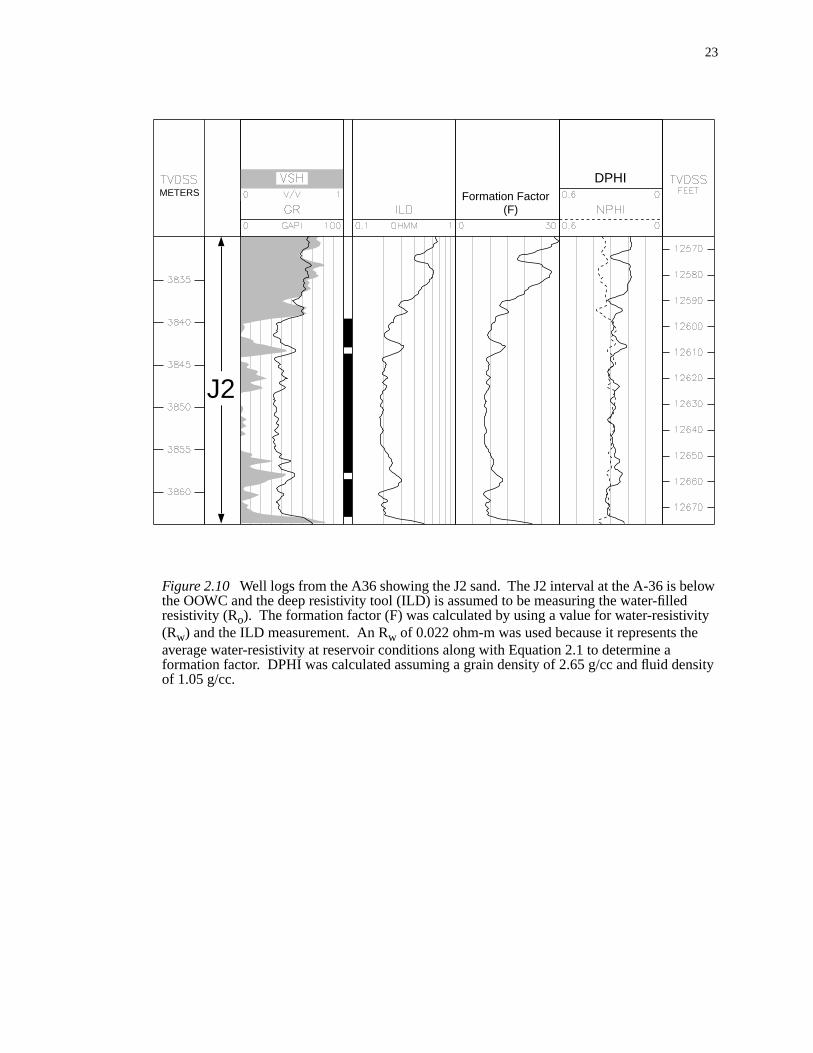
directly from the ILD measurement. In the A36, F ranges from 10 to 30 for the J2 sa

(Figure 2.10).

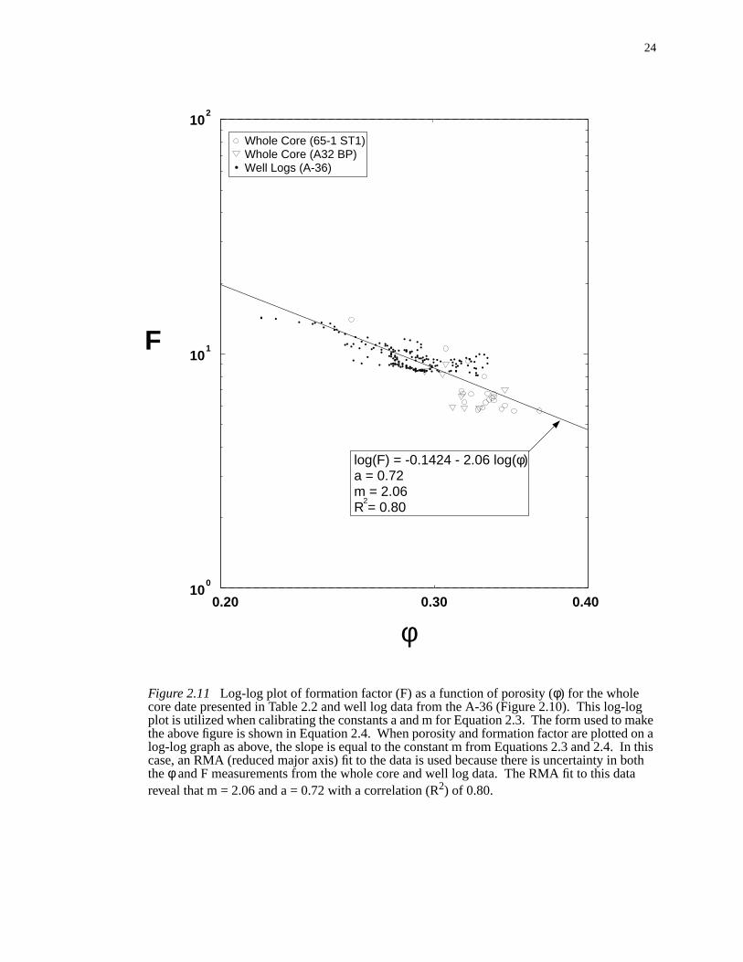
The formation factor (F) was also calculated directly from whole core measurem

from the A32 BP and 65-1 ST1 wells using Equation 2.2 (Table 2.2). For these core

each sample was 100% saturated with brine and its brine-filled resistivity (Ro) was mea-

sured. A brine salinity of 210-230 kppm NaCl was used. The resistivity of the brine

measured at laboratory conditions (75o F) and ranges from 0.0438 to 0.0453 ohm-m. Th

formation factor (F) was then calculated using Equation 2.2 and ranges from 5.71 to

14.00.

Once the formation factor (F) was calculated, the constants a and m were solved f

rearranging Equation 2.3,

. (2.4)

A log-log plot of F vs.φ for the whole core data and the log data from the A36 well revea

that the intercept a = 0.72 and slope m = 2.06 with an R2 of 0.80 (Figure 2.11). These val

ues for a and m are similar to the Humble formula (a = 0.65, m = 2.16; Winsauer et

1952)

F( )log a( )log m φ( )log–=

23

ow

ity

nsity

Figure 2.10 Well logs from the A36 showing the J2 sand. The J2 interval at the A-36 is belthe OOWC and the deep resistivity tool (ILD) is assumed to be measuring the water-filledresistivity (Ro). The formation factor (F) was calculated by using a value for water-resistiv(Rw) and the ILD measurement. An Rw of 0.022 ohm-m was used because it represents theaverage water-resistivity at reservoir conditions along with Equation 2.1 to determine aformation factor. DPHI was calculated assuming a grain density of 2.65 g/cc and fluid deof 1.05 g/cc.

METERSDPHI

J2

Formation Factor (F)

24

logake

on an this bothta

Figure 2.11 Log-log plot of formation factor (F) as a function of porosity (φ) for the wholecore date presented in Table 2.2 and well log data from the A-36 (Figure 2.10). This log-plot is utilized when calibrating the constants a and m for Equation 2.3. The form used to mthe above figure is shown in Equation 2.4. When porosity and formation factor are plottedlog-log graph as above, the slope is equal to the constant m from Equations 2.3 and 2.4. Icase, an RMA (reduced major axis) fit to the data is used because there is uncertainty intheφ and F measurements from the whole core and well log data. The RMA fit to this dareveal that m = 2.06 and a = 0.72 with a correlation (R2) of 0.80.

100

101

102

F

φ0.20 0.30 0.40

Whole Core (65-1 ST1)Whole Core (A32 BP)Well Logs (A-36)

log(F) = -0.1424 - 2.06 log(φ) a = 0.72 m = 2.06 R = 0.80

2

25

t S

rved

satu-

a-

nage

d sat-

tests

e

ly. A

For rocks partially saturated with brine and hydrocarbon, Archie (1942) found thaw

was proportional to the resistivity ratio (I),

, (2.5)

where n is the saturation exponent. The resistivity ratio (I) is defined as

, (2.6)

where Ro is the resistivity of the rock when it is brine-filled and Rt is the resistivity of that

same rock when partially saturated with brine and hydrocarbon. Archie (1942) obse

that for water-wet Gulf Coast sands, n = 2.

Whole core data from both the A32 BP and 65-1 ST1 were used to determine the

ration exponent (n) in cases where Sw and resistivity ratio (I) were measured under labor

tory conditions (Tables 2.3 and 2.4). The data in Table 2.3 were acquired during drai

and imbibition tests on 9 whole core samples. The remaining resistivity index (I) an

uration data used to constrain the saturation exponent (n) were taken under various

and are presented in Table 2.4.

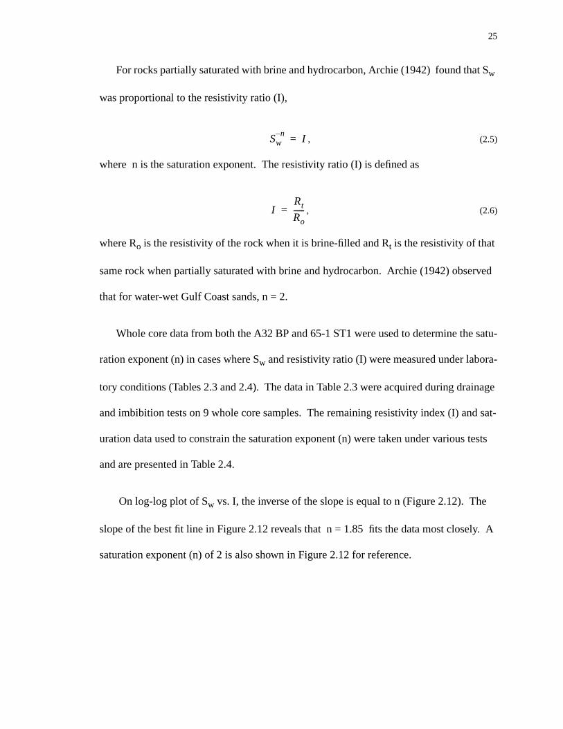
On log-log plot of Sw vs. I, the inverse of the slope is equal to n (Figure 2.12). Th

slope of the best fit line in Figure 2.12 reveals that n = 1.85 fits the data most close

saturation exponent (n) of 2 is also shown in Figure 2.12 for reference.

Swn–

I=

IRt

Ro------=

26

le.l

or n

Figure 2.12 Log-log plot of water saturation (Sw) vs. the resistivity ratio (I) using the whocore data presented in Tables 2.3 and 2.4. The resistivity ratio is defined in Equation 2.5According to Equation 2.5, on a log-log plot of Sw vs. I, the inverse of the slope should be equato the saturation exponent (n). A saturation exponent of 1.85 fit the data. A typical value fis 2 and is shown in the above plot as a comparison.

100

101

102

10−1

100

I

Sw

65 1ST Drainage 65−1ST Imbibition65−1−ST Other A32 BP Drainage A32BP Imbibition A32BP Other

n = 2

n = 1.85

27

t

rchie

tion

gure

ty

in pre-

s

ith

l-

ter

the

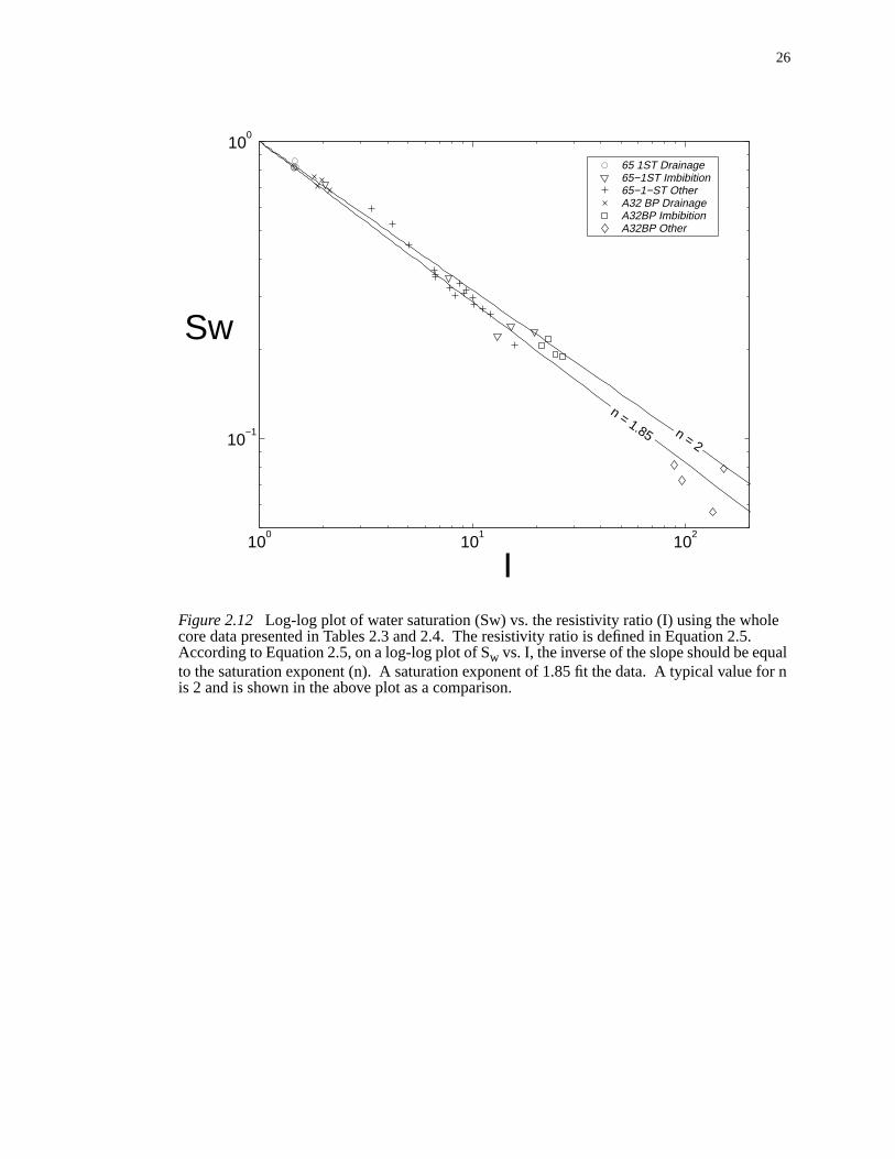
Pickett (1973) combined Equations 2.3 through 2.6 to show how bothφ and Sw affect

Rt:

. (2.7)

On a log-log plot of Rt vs.φ , the water saturation is represented by a series of straigh

lines, all with a slope equal to the constant m. This three-dimensional view of the A

equation shows the sensitivity of log-based Sw calculations to both its measured porosity

and resistivity.

The overall resistivity of a rock is dependent on both the porosity and water satura

(Pickett, 1973; Bhattacharya et al., 1999), as is represented by the Pickett plot in Fi

2.13 . As Rt decreases, the distance between the iso-Sw lines decreases on a Pickett plot.

This reveals that higher Sw, the true resistivity of the rock is more dependent on porosi

rather than Sw. At lower Sw, the distance between the iso-Sw lines in Figure 2.13 is

greater. This suggests that uncertainty in porosity does not severely produce errors

dicted Sw when saturations are at irreducible conditions. Whole core data from Table

2.2, 2.3, and 2.4 are plotted in Figure 2.13. Samples which were 100% saturated w

brine should lie along the Ro line in Figure 2.13, representing a Sw = 1. Samples with dif-

ferent saturations fall within the iso-Sw lines described by Equation 2.7.

The errors associated with the calculation of Sw depend on the uncertainty of the va

ues used for a, m, n,φ, Rw, and Rt (Chen and Fang, 1988). The most important parame

in causing uncertainty in the predicted Sw is the saturation exponent, n. When all of the

parameters (except n) have the same amount of uncertainty, it has been shown that

Rtlog m φlog– aRw( )log n Swlog–+=

28

6.

oreodelter. S

Figure 2.13 Pickett plot constructed using data from Tables 2.2, 2.3,2.4 and Equation 2.When true resistivity (Rt) is plotted vs. porosity (φ) on a log-log scale, the water saturation isrepresented by a family of straight lines. In the above figure, Sw is shown as percent porevolume. At an Sw = 100%, the straight line representing Sw in a Pickett plot is called the Roline and represents how the resistivity of a brine-filled rock depends on porosity. Whole cdata measured at various saturations are plotted to show the overall quality of the Archie mused for calculating saturation. The blue circles represent rocks saturated with 100% waThe yellow triangles, for example, represent rocks whose resistivity was measured with awranging from 5 to 10 percent.

Sw = 5 to 10 Sw = 10 to 20 Sw = 20 to 30

Sw = 30 to 40 Sw = 40 to 50 Sw = 50 to 60

Sw = 60 to 70 Sw = 70 to 80 Sw = 80 to 90

Sw = 100

10−1

100

101

5102030405060708090

0.25

0.40

Ro Line

a = 0.72 m = 2.06 n = 1.85

0.30

φ

R (ohm-m)t

29

s

ween

s

ppro-

ions

r

The

osity,

on

ri-

he J1

constant m is the most important variable in causing errors in Sw, followed byφ, a, Rw, and

Rt (Chen and Fang, 1988).

The method used here to calculated the uncertainty is to use the Archie equation

along with the calibrated constants (a = 0.72, m = 2.06, n = 1.85) to predict Sw based

solely on the measured whole core porosity (Tables 2.3 and 2.4). The rms error bet

the predicted Sw and measured Sw was then taken as the uncertainty. Figure 2.14 show

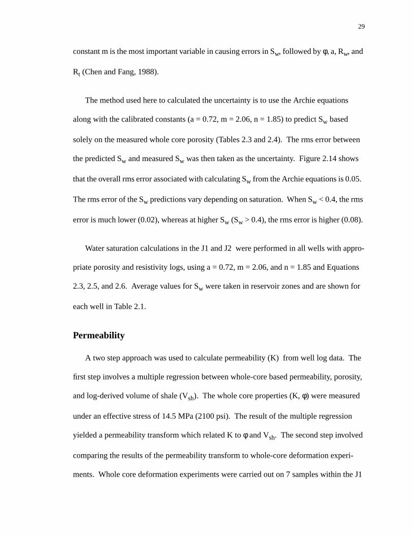
that the overall rms error associated with calculating Sw from the Archie equations is 0.05.

The rms error of the Sw predictions vary depending on saturation. When Sw < 0.4, the rms

error is much lower (0.02), whereas at higher Sw (Sw > 0.4), the rms error is higher (0.08).

Water saturation calculations in the J1 and J2 were performed in all wells with a

priate porosity and resistivity logs, using a = 0.72, m = 2.06, and n = 1.85 and Equat

2.3, 2.5, and 2.6. Average values for Sw were taken in reservoir zones and are shown fo

each well in Table 2.1.

Permeability

A two step approach was used to calculate permeability (K) from well log data.

first step involves a multiple regression between whole-core based permeability, por

and log-derived volume of shale (Vsh). The whole core properties (K,φ) were measured

under an effective stress of 14.5 MPa (2100 psi). The result of the multiple regressi

yielded a permeability transform which related K toφ and Vsh. The second step involved

comparing the results of the permeability transform to whole-core deformation expe

ments. Whole core deformation experiments were carried out on 7 samples within t

30

d

MS

Figure 2.14 Predicted Sw vs. measured Sw when a = 0.72, n = 1.85, and m = 2.06. The dasheline shows a one-to-one correlation. This model was used to calculate Sw from the porosity andresistivity (Rt) data in Tables 2.3 and 2.4. The RMS error was calculated between thepredicted and measured saturations. For all of the data, the RMS error was 0.05. The Rerror was lower at Sw < 0.4 and equals 0.02. At higher Sw (Sw > 0.4) the RMS error was 0.08.

Pre

dict

ed S

w

Measured Sw

a = 0.72 m = 2.06 n = 1.85

rms Error all points = 0.05 Sw < 0.4 = 0.02 Sw > 0.4 = 0.08

31

he

lus-

32

(Fig-

eir

atu-

ever,

well

the

orer

t

and J2 and relate the porosity loss through compaction to permeability reduction. T

advantage of these experiments are that they allow us to track the K,φ behavior of a single

sample whose Vsh is constant.

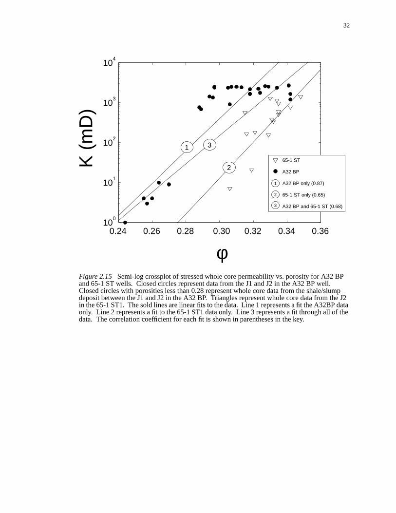
Porosity alone is a poor predictor for permeability in the J1 and J2 sands, as is il

trated with whole core data from the A32 BP and 65-1 ST wells (Figure 2.15). The A

BP data show a wide range of porosities for any given permeability above 1000 mD

ure 2.15). Permeability for the 65-1 ST samples are generally lower, even though th

porosities are not below 0.30.

Factors which control permeability include grain size, sorting, irreducible water s

ration, porosity, and shale content (Timur, 1968; Hearst, 1996; Veranda, 1999). How

not all of these factors (grain size and sorting) are directly obtainable from open-hole

log analysis. Porosity and Vsh, however, are readily available from openhole well log

analysis and are used to predict horizontal and vertical permeability where K =f(φ,Vsh):

(2.8)

Equation 2.8, although not explicitly, takes into account grain size and sorting through

Vsh term. Rocks can have the same porosity but different grainsizes. Rocks with po

sorting and smaller grain sizes tend to have higher Vsh and lower permeability, while a

cleaner sand with the same porosity may have low Vshhave higher permeability (Hearst e

al., 1996; Vernik, 2000).

K 10A B φ( )log CVsh+ +[ ]

=

32

P

mp the J2data

f the

Figure 2.15 Semi-log crossplot of stressed whole core permeability vs. porosity for A32 Band 65-1 ST wells. Closed circles represent data from the J1 and J2 in the A32 BP well.Closed circles with porosities less than 0.28 represent whole core data from the shale/sludeposit between the J1 and J2 in the A32 BP. Triangles represent whole core data fromin the 65-1 ST1. The sold lines are linear fits to the data. Line 1 represents a fit the A32BPonly. Line 2 represents a fit to the 65-1 ST1 data only. Line 3 represents a fit through all odata. The correlation coefficient for each fit is shown in parentheses in the key.

0.24 0.26 0.28 0.30 0.32 0.34 0.3610

0

101

102

103

104

K (

mD

)

φ

1

2

3

65-1 ST

A32 BP

A32 BP only (0.87)

65-1 ST only (0.65)

A32 BP and 65-1 ST (0.68)

1

2

3

33

d in

. A

ws

.9

V

y

and

is

rease

han

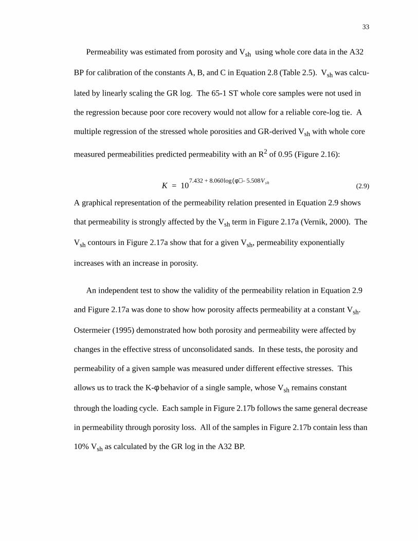
Permeability was estimated from porosity and Vsh using whole core data in the A32

BP for calibration of the constants A, B, and C in Equation 2.8 (Table 2.5). Vshwas calcu-

lated by linearly scaling the GR log. The 65-1 ST whole core samples were not use

the regression because poor core recovery would not allow for a reliable core-log tie

multiple regression of the stressed whole porosities and GR-derived Vsh with whole core

measured permeabilities predicted permeability with an R2 of 0.95 (Figure 2.16):

(2.9)

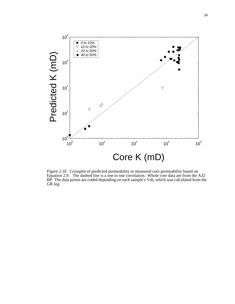
A graphical representation of the permeability relation presented in Equation 2.9 sho

that permeability is strongly affected by the Vshterm in Figure 2.17a (Vernik, 2000). The

Vsh contours in Figure 2.17a show that for a given Vsh, permeability exponentially

increases with an increase in porosity.

An independent test to show the validity of the permeability relation in Equation 2

and Figure 2.17a was done to show how porosity affects permeability at a constant sh.

Ostermeier (1995) demonstrated how both porosity and permeability were affected b

changes in the effective stress of unconsolidated sands. In these tests, the porosity

permeability of a given sample was measured under different effective stresses. Th

allows us to track the K-φ behavior of a single sample, whose Vsh remains constant

through the loading cycle. Each sample in Figure 2.17b follows the same general dec

in permeability through porosity loss. All of the samples in Figure 2.17b contain less t

10% Vsh as calculated by the GR log in the A32 BP.

K 107.432 8.060 φ( )log 5.508Vsh–+

=

34

e A32m the

Figure 2.16 Crossplot of predicted permeability to measured core permeability based onEquation 2.9. The dashed line is a one to one correlation. Whole core data are from thBP. The data points are coded depending on each sample’s Vsh, which was calculated froGR log.

100

101

102

103

104

100

101

102

103

104

Pre

dict

ed K

(m

D)

0 to 10%10 to 20%20 to 30%40 to 50%

Core K (mD)

35

orehole

s intoplesility is

Figure 2.17 Permeability transform presented in Equation 2.9 based on stressed whole cdata from the A32 BP (Table 2.5). Contours in both a) and b) are iso-Vsh lines. a) The wcore data are plotted with different symbols, depending on Vsh. Vsh for each whole coresample was taken by linearly scaling the GR log. The above permeability transform takeaccount both porosity and Vsh. b) Porosity and permeability for several whole core samwhich were measured under increasing effective stress. These data show how permeabreduced by changing the porosity under stress while at a constant value of Vsh.

0.24 0.26 0.28 0.30 0.32 0.34 0.36

0

1

2

3

10

10

10

10

104

K (

mD

)

φ

0

0.1

0.2

0.3

0.4

0.5

0.6

0 to 10%10 to 20%20 to 30%40 to 50%

0

1

2

3

10

10

10

10

104

0.26 0.30 0.34 0.380.22 0.40

0

0.1

0.2

0.3

0.4

0.5

0.6

16192133465156

Sample #

K (

mD

)

φ

a)

b)

Vsh

Vsh

36

ined

BP

e AS

J2

tur-

ini-

the J1

2 BP,

ed GR

high

the

the

sepa-

, as

fan

Geologic Model

Facies and Depositional Environments

Amalgamated Sheet Sand (AS)

The AS facies has a blocky GR and ILD log signature and is very fine to fine gra

(14% silt and clay, 45% fine, 22% very fine, 19% medium grain by weight). The A32

penetrated the J2 (Figure 2.18a) and J1 (Figure 2.19a) within a typical example of th

facies. Sand thickness in the AS facies ranges from 20 to 30 m (70 to 100 ft) in the

and 10 to 12 m (30 to 40 ft) in the J1 with a typically high net-to-gross of 98%.

The depositional environment of the AS facies is within the proximal portion of a

bidite fan. Multiple turbidites may pond themselves in a subsiding salt-withdrawal m

basin, depositing large amounts of sands in the form of sheets. The sheet sands in

and J2 are laterally continuous and are found to be amalgamated in the area of the A3

A4BP, and A38 (Figures 2.18 and 2.19).

Layered Sheet Sand (LS)

The AS facies grades into a layered and shale prone facies that has an interbedd

and ILD signature (Figure 2.20). Clean sands within the LS facies have low GR and

ILD values while the interbedded shales have lower GR and ILD values as shown in

65-1 (Figure 2.18c). Although net to gross is lower in the LS than AS facies (70%),

65-1 does contain several clean sand layers, typically 0.5 to 10 m (3 to 30 ft) thick,

rated by shales.

The LS facies is interpreted to record deposition at the distal portion of the fan lobe

opposed to the AS facies, which represents deposition in the proximal portion of the

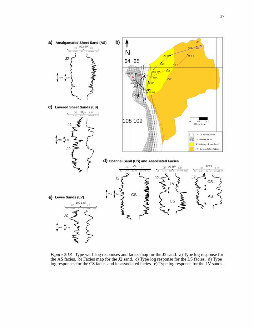
37

e for) Typesands.

Figure 2.18 Type well log responses and facies map for the J2 sand. a) Type log responsthe AS facies. b) Facies map for the J2 sand. c) Type log response for the LS facies. dlog responses for the CS facies and its associated facies. e) Type log response for the LV

65

109108

64

0 0.5 1.0(Kilometers)

N

CS - Channel Sands

LV - Levee Sands

AS - Amalg. Sheet Sands

LS - Layered Sheet Sands

A5 BP

A36109-1

A32 BP

A2 BP

A38

A10

A4 BP 65-1 ST

A60 65-1

A9

A

A’

B’

B

109-1 ST1 A1

A35

A11 BP

A41

A33

A31

A34

A37

A3 BP5 m20 ft

J2

A32 BPAmalgamated Sheet Sand (AS)a)

Layered Sheet Sands (LS)65-1

5 m20 ft

J1

J2

c)

5 m20 ft

J2

CS

A1

J2

LV

CS

A3 BP 109-1

CS

AS

J2

Channel Sand (CS) and Associated Facies d)

5 m20 ft

J2

109-1 ST

Levee Sands (LV)e)

b)

C

C’

D’

D

38

e forcies.

the J1

Figure 2.19 Type well log responses and facies map for the J1 sand. a) Type log responsthe AS facies. b) Type log response for the LV facies. c) Type log response for the LS fad) Type log responses for the CS facies and its associated LV facies. e) Facies map for sand.

5 m20 ft AS

J1

A32 BP

Amalgamated Sheet Sand (AS)a)

J2

65-1

5 m20 ft

J1

Layered Sheet Sands (LS)c)

A33

5 m20 ft

J1

Levee Sands (LV) b)

5 m20 ft

J1

CS

LV

A1

Channel Sands (CS)d)

A-1

J2

65-1

5 m20 ft

J1

A-1

A31

A33

A32 BP

A38

A10

A9

A38 ST

A4 BP

65-1 ST

A60 65-1

A35

A11 BP

A3 BP A1

A41

A37

65

109108

64 0 0.5 1.0(Kilometers)

N

A34

A5 BP

109-1

A2 BP

A

A’

B’

B

109-1ST

CS - Channel Sands

LV - Levee Sands

AS - Amalg. Sheet Sands

LS - Layered Sheet Sands

e)

C

C’D’

D

39

-B’

low

Figure 2.20 Cross sections flattened on the bottom of the J2 horizon for lines A-A’ and B(Figure 2.18) showing facies relationships. For each well, a GR (left) and ILD (right) areshown. Some wells (A-10, 65-1-ST1) penetrated the J2 sand below the OWC and have ILD values. The color scheme denotes different facies within the J1 and J2. Erosionalunconformities are named Cuts 1 through 3.

00.5

1

Kilom

eters

109-1ST

A3 B

PA

37A

1

109-1A

1065-1S

T1

65-1

J3 J2 J1J1

Cut 3

Cut 1

Cut 2

LS - Layered S

heet

AS

- Am

alg. Sheet

CS

- Channel

LV - Levee

AA

’

A34

A2 B

P109-1

A32 B

PA

38A

4 BP

65 1

J1J2C

ut 1

Cut 3

J3

BB

’

100 ft30 m

100 ft30 m

40

sition

rgins

o-

y a

S

e CS

erly-

and

109-

and

ity in

ells

nd J2

other

. The

(Figures 2.18 and 2.20). The interbedded shale layers represent hemipelagic depo

in between flow events and debris slumps which more than likely came from the ma

of the rapidly filling Bullwinkle basin (Holman and Robertson, 1994).

Channel Sand (CS)

The Channel facies (CS) of the J2 in general contains thick sands with sharp, er

sional contacts with the beds they overlie. In some cases, the CS facies is capped b

thinner LV facies within the J1 and J2 (Figures 2.18 and 2.19). Within the J2, the C

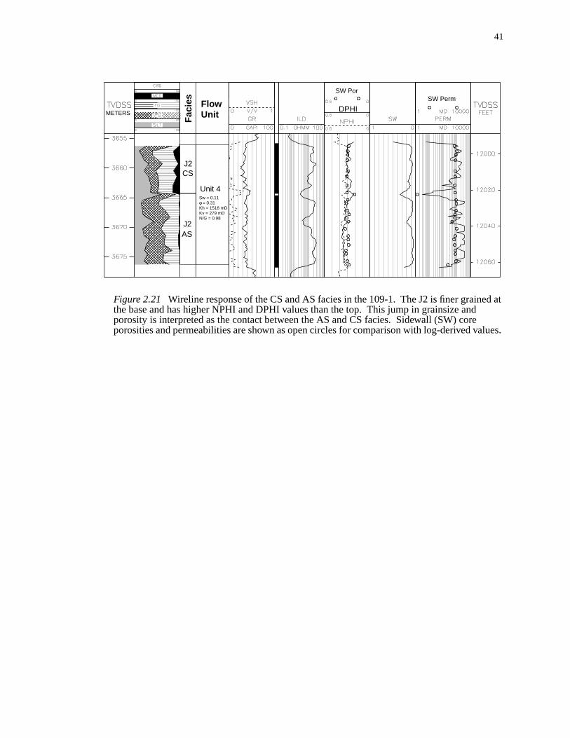
facies may also overlie the AS facies (109-1 in Figure 2.21). The thickest part of th

facies in the J2 are in the A1, A37, and A31 wells, where it is interpreted that the und

ing AS facies has been entirely removed by channel erosion (Figure 2.20).

The AS facies is distinguished from the CS facies by a sharp increase in grain size

decrease in porosity. An example of this is in the 109-1 (Figure 2.21). The CS in the

1 is coarser grained (fine to medium) than the underlying AS facies and both DPHI

NPHI logs record a higher porosity in AS (~0.33) than the CS facies (~0.29). Poros

the AS facies is slightly greater than in the CS facies for the A34, A2BP, and A5 BP w

(Figure 2.20).

The CS facies is interpreted to result from channels which swept across the J1 a

AS facies. These channels cut into the underlying AS facies in some places, and in

places removed the AS facies completely, cutting into the shales above the J2 sand

CS facies in the J1 and J2 are found in the western portion of the field.

41

d at

lues.

Figure 2.21 Wireline response of the CS and AS facies in the 109-1. The J2 is finer grainethe base and has higher NPHI and DPHI values than the top. This jump in grainsize andporosity is interpreted as the contact between the AS and CS facies. Sidewall (SW) coreporosities and permeabilities are shown as open circles for comparison with log-derived va

J2CS

Unit 4Sw = 0.11φ = 0.31Kh = 1518 mDKv = 279 mDN/G = 0.98

SW PorSW Perm

METERS

Fac

ies

FlowUnit

ASJ2

DPHI

42

cies

. The

ure

ch

orm

ture is

e

her

d

.

t and

basin

on-

(LS).

by the

s of

Levee (LV)

There is also evidence for a levee/overbank (LV) facies associated with the CS fa

in the J2 in the 109-1 ST well (Figure 2.18 and Figure 2.19). The LV facies is finer

grained than the CS facies and contains 5 to 10 ft thick sands interbedded with shales

LV facies in some places overlie a thick CS facies (A3BP in Figure 2.18 and A37 in Fig

2.20).

The LV facies is interpreted to be deposited on the overbanks of the channel whi

swept across the J1 and J2 sands.

Geologic Evolution

Deposition of the J Sand package occurred in a salt withdrawal mini-basin in the f

of turbidite sheets and channels (Holman and Robertson, 1994). The stratal architec

similar to other deepwater Gulf of Mexico fields where primary deposition of turbidit

sheet sands within actively subsiding salt withdrawal minibasins was followed by hig

energy channel cutting and deposition after salt withdrawal had stopped (Holman an

Robertson, 1994; Prather et al., 1998; Hoover et al., 1999; Winker and Booth, 2000)

Early time deposition of the J2 sands was in the form of both amalgamated shee

layered sheet sands (Figures 2.18 and 2.20) which may have been directed into the

from the west by salt-cored bathymetric highs (Winker and Booth, 2000). This envir

ment was divided into two lithofacies: the amalgamated sheet (AS) and layered sheet

These sheets are laterally continuous across the field in the J2 and are represented

A32 BP, A4BP, A10, and A38 in Figure 2.20. The AS facies grades into the LS facie

the 65-1 and 65-1 ST to the east.

43

acies

is

sands

J2 CS

The

annel

e field

re

5 BP

out

(Fig-

ies

more

n of

ck to

n

in the

s in

quent

the

The J2 AS facies was cut by a subsequent channel (Cut 1, Figure 2.20). The CS f

in the J2 records a channel that flowed across the Bullwinkle basin (Figure 2.18). It

interpreted that there was no longer any accommodation space available to pond the

and as a result, the channel cut into the underlying deposits. The coarse base in the

facies in the 109-1 (Figure 2.21) may record a lag deposit (Beaubouef et al., 1999).

LV facies in the J2 record levee/overbank deposits which were associated with the ch

that swept across the J2. The LV facies is more prevalent on the western edge of th

where it was penetrated in the J2 in the A11BP, 109-1 ST, A41, and A33 wells (Figu

2.18). Some evidence for the LV facies was also recorded farther to the east in the A

where it overlies a thick section of CS facies. A west-to-east pattern of LV facies pinch

may indicate that the channel started cutting in the western edge of the field initially

ure 2.20). The channel then moved farther east, where it cut into the LV and AS fac

which were already present in the J2 and preserved the LV facies in the west

Subsidence and salt uplift during J2 channel sand cutting and deposition created

accommodation in the Bullwinkle basin (Holman and Robertson, 1994). The creatio

accommodation changed sand deposition from channel-style facies (CS and LV) ba

sheet in the J1 (AS and DS facies in Figures 2.19 and 2.20). Deposition of the J1 i

bathymetric lows occurred in the same way as J2, where AS facies were deposited

western edge of the field (109-1ST, A-10, A32 BP, A38 in Figure 2.19). The LS facie

the J1 was deposited in the distal part of the fan on the eastern edge of the field.

A bypass phase in the J1 led to erosion (Cut 2) of the J1 sheet sands and subse

deposition of CS and LV facies (Figure 2.20). The J1 channel/levee system cut into

44

nica-

the

osion

when

moda-

d the

998;

m-

20).

til sea

tson,

a-

envi-

e

ger

on

re

nt

uds

top of the J2 in some places (A37 in Figure 2.20) and made updip hydraulic commu

tion between the J1 and J2 possible. Unlike the J2, the AS facies was preserved to

east of the channel in the J1. (109-1ST in Figure 2.20).

Subsequent changes in either sea level or sediment supply eventually caused er

of the top of the J Sand package (Cut 3 in Figure 2.20). This bypass phase occured

there was no longer accommodation space left for sediment amalgamation. Accom

tion space was no longer created because the sediment accumulation rate exceede

rate at which the salt could deform (Holman and Robertson, 1994; Prather et al., 1

DeVay et al., 2000; Winker and Booth, 2000) The J1 in some places is bifurcated co

pletely and some of the cutting extends down to the top of the J2 (109-1 in Figure 2.

Channel/levee systems continually migrated across the top of the J Sand package un

level rose once again and the basin returned to a bathyl setting (Holman and Rober

1994).

Implications for Production and Sand Connectivity

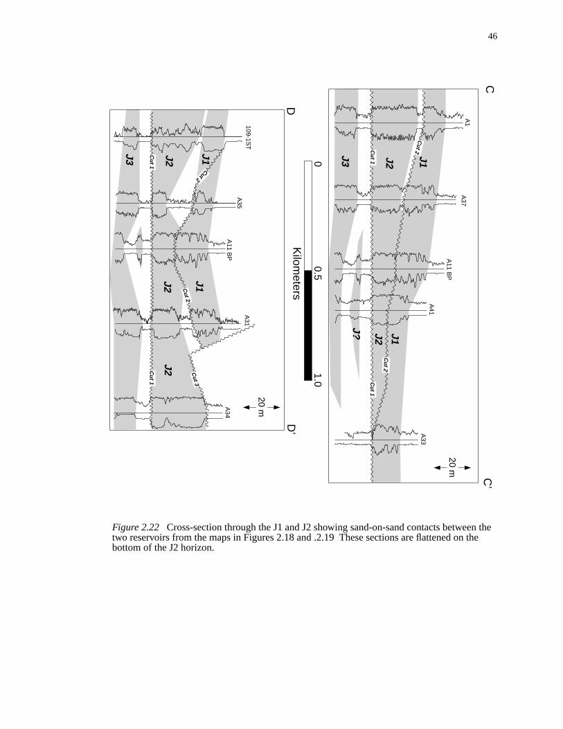
Initially, all 4 of the J Sands (J1 through J4) were thought to be hydraulically sep

rated, due to the highly continuous nature of the sands and shales in the AS and LS

ronment (Holman and Robertson, 1994). The LS and AS facies of the J1 and J2 ar

similar to the facies described by McGee et al. (1994) and Kendrick (2000) in the Au

Field (Figure 2.4). There is a high degree of correlation of sands between wells and

seismic in the Auger field, indicating that sands and muds in the AS and LS facies a

highly continuous. Individual sands and reservoirs within the AS and LS environme

should show very little, if any, vertical communication between reservoirs, since the m

45

e

ta

s are

rvoir

g and

epo-

thick

te

te

op of

sional

ical

s a

t into

ars

).

Lower

are

bounding them are also continuous. This model was initially used when planning th

development of the Bullwinkle J Sands (Holman and Robertson, 1994). Pressure da

from subsequent development wells, however, show quite clearly that all of the J Sand

indeed connected and are in hydraulic communication, effectively acting as one rese

(Holman and Robertson, 1994).

Hydraulic communication between the J1 and J2 is a result of the channel cuttin

in-filling occurring during the deposition of the J1 (Figure 2.22). At the close of J2 d

sition, hemipelagic deposition and slumps from the margins of the basin covered the

sands of the J2 with muds and hydraulically separated them any subsequent turbidi

sheets. The AS and LS facies deposited in the J1 were initially hydraulically separa

from the J2. Subsequent erosion during deposition of the J1 CS facies cut into the t

the J2, making vertical communication between the two sands possible across an ero

unconformity (Cut 2 in Figure 2.22). There is evidence from well data showing a vert

sand-on-sand contact between the J1 and J2 in the A11 BP and A41 wells. There i

north to south deepening of the erosional unconformity at the base of the J1 which cu

the younger shales and J2 sand below (Figures 2.20b and 2.22).

Comparison with Other Deepwater Gulf of Mexico Fields

Another Gulf of Mexico analog similar to the Bullwinkle J1 and J2 sands is the M

field in Mississippi Canyon Block 807, which is described in detail by Mahaffie (1994

The Mars field contains several sheet and channel sand reservoirs. The Upper and

Yellow intervals at Mars are very similar to the Bullwinkle J1 and J2 sands in that they

46

n thethe

Figure 2.22 Cross-section through the J1 and J2 showing sand-on-sand contacts betweetwo reservoirs from the maps in Figures 2.18 and .2.19 These sections are flattened on bottom of the J2 horizon.

A37

A1

A11 B

P

A41

A33

J2 J1

J1J2

J300.5

1.0

Kilom

eters

J?

CC

’

Cut 1

Cut 2

Cut 1

Cut 2

109-1ST

A35

A11 B

P

A31

A34

DD

’

J2

J1J3

J2J2

Cut 1

Cut 1

Cut 2

Cut 2

Cut 3

J1

20 m

20 m

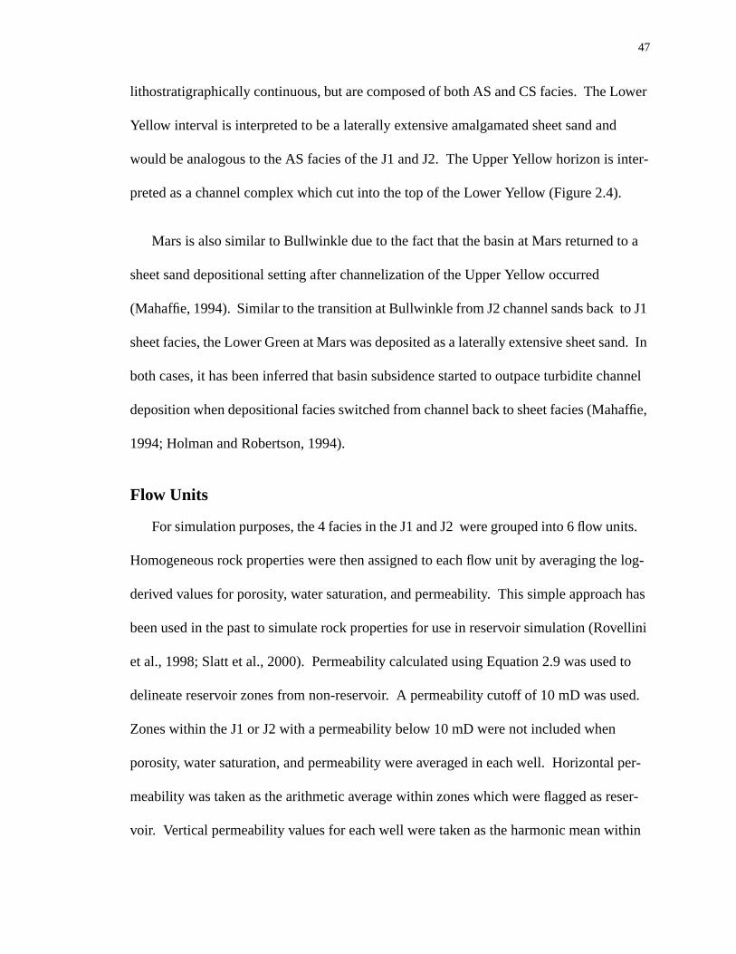
47

wer

d

inter-

o a

J1

nd. In

hannel

affie,

its.

e log-

h has

ellini

to

ed.

per-

ser-

thin

lithostratigraphically continuous, but are composed of both AS and CS facies. The Lo

Yellow interval is interpreted to be a laterally extensive amalgamated sheet sand an

would be analogous to the AS facies of the J1 and J2. The Upper Yellow horizon is

preted as a channel complex which cut into the top of the Lower Yellow (Figure 2.4).

Mars is also similar to Bullwinkle due to the fact that the basin at Mars returned t

sheet sand depositional setting after channelization of the Upper Yellow occurred

(Mahaffie, 1994). Similar to the transition at Bullwinkle from J2 channel sands back to

sheet facies, the Lower Green at Mars was deposited as a laterally extensive sheet sa

both cases, it has been inferred that basin subsidence started to outpace turbidite c

deposition when depositional facies switched from channel back to sheet facies (Mah

1994; Holman and Robertson, 1994).

Flow Units

For simulation purposes, the 4 facies in the J1 and J2 were grouped into 6 flow un

Homogeneous rock properties were then assigned to each flow unit by averaging th

derived values for porosity, water saturation, and permeability. This simple approac

been used in the past to simulate rock properties for use in reservoir simulation (Rov

et al., 1998; Slatt et al., 2000). Permeability calculated using Equation 2.9 was used

delineate reservoir zones from non-reservoir. A permeability cutoff of 10 mD was us

Zones within the J1 or J2 with a permeability below 10 mD were not included when

porosity, water saturation, and permeability were averaged in each well. Horizontal

meability was taken as the arithmetic average within zones which were flagged as re

voir. Vertical permeability values for each well were taken as the harmonic mean wi

48

in the

hile

teris-

3

Hor-

e of

AS

ough

sent

)

osity

has

t 1

abil-

er

due

ue of

the reservoir zones. Porosity and water saturation were taken as the arithmetic mean

reservoir zones. Table 2.6 is a summary of each flow unit’s petrophysical properties, w

Table 2.1 shows the average petrophysical properties for each well.

Unit 1 contains the AS facies of the J2 sand and overall has the best flow charac

tics (Figure 2.23). Three wells penetrated Unit 1, with the A32 BP showing the log-

derived petrophysical properties (Figure 2.25). Porosity has an average value of 0.3

(Table 2.6). Water saturation ranges from 0.14 to 0.18 with an average value of 0.16.

izontal permeability is excellent, ranging from 2300 to 2500 mD with an average valu

2400 mD. Vertical permeability is approximately 50% of the horizontal permeability,

with an average value of 1100 mD. The high vertical permeability is the result of the

facies high net-to-gross (0.99) within Unit 1.

Unit 2 contains the LS facies of the J1 and J2 sands (Figures 2.23 and 2.24). Alth

the LS facies contains many interbedded sands and shales, the sands which are pre

have decent flow properties. Three wells penetrated Unit 2, although only one (65-1

logged above the OOWC in the J1 and J2 (Figure 2.26). Table 2.6 indicates that por

ranges from 0.29 to 0.32 with an average value of 0.30. Water saturation in the 65-1

an average value of 0.20. Horizontal permeability is lower than the AS facies of Uni

and ranges from 724 to 1355 mD with an average value of 1056 mD. Vertical perme

ity ranges from 82 to 226 mD with an average value of 155 mD. Although the clean

sands in Unit 2 have excellent reservoir properties, the lower vertical permeability is

to the interbedded nature of the LS facies. Overall, net-to-gross has an average val

0.74.

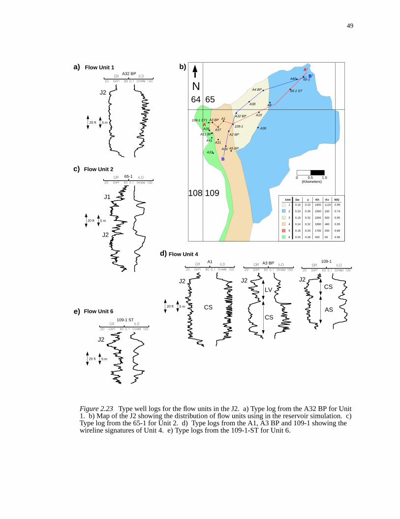
49

it. c)he

Figure 2.23 Type well logs for the flow units in the J2. a) Type log from the A32 BP for Un1. b) Map of the J2 showing the distribution of flow units using in the reservoir simulationType log from the 65-1 for Unit 2. d) Type logs from the A1, A3 BP and 109-1 showing twireline signatures of Unit 4. e) Type logs from the 109-1-ST for Unit 6.

5 m20 ft

J2

A32 BPFlow Unit 1a)

Flow Unit 265-1

5 m20 ft

J1

J2

c)

5 m20 ft

J2

CS

A1

J2

LV

CS

A3 BP 109-1

CS

AS

J2

Flow Unit 4 d)

5 m20 ft

J2

109-1 ST

Flow Unit 6e)

b)

65

109108

64

0 0.5 1.0(Kilometers)

N

109-1 ST1 A1

A35

A11 BP

A41

A33

A31

A34

A37

A5 BP

A36

A3 BP

109-1

A32 BP

A2 BP

A38

A10

A4 BP 65-1 ST

A60 65-1

A9

A

A’

B’

B

1 0.16 0.33 2400 1120 0.99

2 0.20 0.30 1060 160 0.74

3 0.19 0.32 2260 920 0.95

4 0.14 0.32 1890 460 0.93

5 0.16 0.33 1700 200 0.69

6 0.25 0.28 420 50 0.56

Unit Sw φ Kh Kv N/G

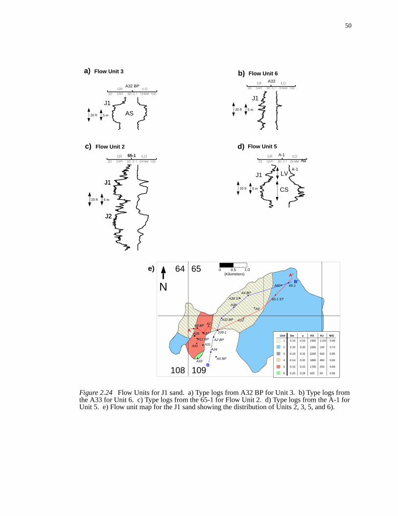
50

mr

Figure 2.24 Flow Units for J1 sand. a) Type logs from A32 BP for Unit 3. b) Type logs frothe A33 for Unit 6. c) Type logs from the 65-1 for Flow Unit 2. d) Type logs from the A-1 foUnit 5. e) Flow unit map for the J1 sand showing the distribution of Units 2, 3, 5, and 6).

5 m20 ft AS

J1

A32 BP

Flow Unit 3a)

J2

65-1

5 m20 ft

J1

Flow Unit 2c)

A33

5 m20 ft

J1

Flow Unit 6b)

5 m20 ft

J1

CS

LV

A1

Flow Unit 5d)

A-1

J2

65-1

5 m20 ft

J1

A-1

e)

A31

A33

A32 BP

A38

A10

A9

A38 ST

A4 BP

65-1 ST

A60 65-1

A35

A11 BP

A3 BP A1

A41

A37

65

109108

64 0 0.5 1.0(Kilometers)

N

A34

A5 BP

109-1

A2 BP

A

A’

B’

B

1 0.16 0.33 2400 1120 0.99

2 0.20 0.30 1060 160 0.74

3 0.19 0.32 2260 920 0.95

4 0.14 0.32 1890 460 0.93

5 0.16 0.33 1700 200 0.69

6 0.25 0.28 420 50 0.56

Unit Sw φ Kh Kv N/G

51

filledsingn 2.9ed

Figure 2.25 Well logs for the A32 BP AS facies showing the relationship between wirelineresponse, facies, and flow units. The black bars represent areas in the J1 and J2 withpermeabilities exceeding 10 mD. Open circles are sidewall (SW) core measurements andcircles are whole core (WC) measurements. DPHI in the porosity track was calculated uEquation 2.1 and a fluid density of 0.98 g/cc. Permeability was calculated using Equatioand the Vshcurve next to the GR log. An upper limit of 3500 mD was chosen for the log-baspermeability prediction.

J1AS

J2AS

Sw = 0.16φ = 0.33Kh = 2315 mDKv = 1122 mDN/G = 0.99

Unit 1


SW Por

WC Por

DPHIWC Perm

SW Perm

METERS Fac

ies

Flow Units

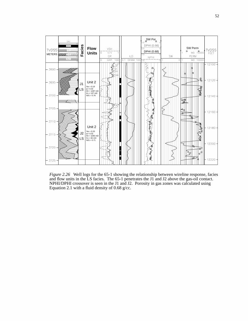
52

iestact.ing

Figure 2.26 Well logs for the 65-1 showing the relationship between wireline response, facand flow units in the LS facies. The 65-1 penetrates the J1 and J2 above the gas-oil conNPHI/DPHI crossover is seen in the J1 and J2. Porosity in gas zones was calculated usEquation 2.1 with a fluid density of 0.68 g/cc.

J1

LS


SW Por

SW Perm

METERS Fac

ies

Flow Units

Sw = 0.20φ = 0.32Kh = 1093 mDKv = 82 mDN/G = 0.71

LS

J2

Unit 2

DPHI (0.98)

DPHI (0.68)

53

ry

me-

ly

age

of

ces

only

the

ies in

igh

32

Hor-

e

ith

es-

.98

CS

J1

ble

Unit 3 contains the AS facies of the J1 sand (Figures 2.24 and 2.25). Unit 3 is ve

similar in reservoir properties to the AS facies in Unit 1. Porosity and horizontal per

ability are comparable with Unit 1, with average values of 0.32 and 2260, respective

(Table 2.6). Unit 2 exhibits a slightly higher water saturation than Unit 1, with an aver

value of 0.19. Vertical permeability is also comparable with Unit 2, being about 50%

the horizontal permeability.

Unit 4 is largely made up of the CS facies of the J2, although it includes in some pla

the LV and AS facies. The A3 BP well shows an example in Unit 4 where a thick CS

facies is present below thinner LV facies (Figure 2.23). The A1 is an example where

thick, clean CS facies is present (Figure 2.23). The 109-1 well is an example where

CS facies is present above the AS facies (Figures 2.21 and 2.23). The rock propert

Unit 4 show some variability in terms of saturation and permeability, but overall it is h

quality reservoir rock. Porosity ranges from 0.31 to 0.33 with an average value of 0.

(Table 2.1). Water saturation varies from 0.08 to 0.19 with an average value of 0.14.

izontal permeability is highly variable, ranging from 1500 to 2200 mD with an averag

value of 1889 mD. Vertical permeability is about 25% of the horizontal permeability, w

an average value of 459 mD. The low vertical permeability in Unit 4 is due to the pr

ence of LV sands in some wells. Net-to-gross is still very high, ranging from 0.77 to 0

with an average value of 0.93.

The CS and LV facies in the J1 are grouped into Unit 5 and are distinct from the

and LV facies in Unit 4 in that Unit 5 exhibits an overall lower net-to-gross (0.69). The

sand in the A-1 well shows an example of Unit 5 (Figure 2.24). Porosity is compara

54

tal

erti-

erti-

nds

Fig-

n the

ple of

8

e of

nit 6

e to

value

with Unit 4 and has an average value of 0.33 (Table 2.6). Water saturation is slightly

higher than Unit 4, ranging from 0.13 to 0.22 with an average value of 0.16. Horizon

permeability ranges from 1495 mD to 1981 mD with an average value of 1715 mD. V

cal permeability is lower than Unit 4, with an average value of 211 mD. The lower v

cal permeability is the result of Unit 5 containing more wells with both CS and LV sa

present than Unit 4.

Unit 6 contains the low quality reservoir sands of the LV facies in the J1 and J2 (

ures 2.23 and 2.24). LV type facies are known to have poorer reservoir qualities tha

CS facies of Units 4 and 5 (Bourgeois et al., 1996). The 109-1-ST shows an exam

Unit 6 (Figure 2.27). Porosity ranges from 0.26 to 0.30 with an average value of 0.2

(Table 2.1). Water saturation is high, ranging from 0.20 to 0.35 with an average valu

0.25. Horizontal permeability in some places reaches as high as 990 mD, although U

has an average of 421 mD. Vertical permeability is extremely low compared with the

other flow units, with an average value of 52 mD. The low vertical permeability is du

the interbedded nature of the LV facies in Unit 6, where net-to-gross has an average

of 0.56.

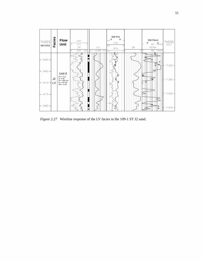
55

Figure 2.27 Wireline response of the LV facies in the 109-1 ST J2 sand.

J2LV


SW PorSW Perm

METERS Fac

ies

FlowUnit

56

og

dep-

nds.

of

in the

n

h made

re

its for

ich

nnels

.

erties

Conclusions

We formulated a depositional and reservoir simulation model based on wireline l

interpretation for the J1 and J2 sands. Facies identification from well logs aided in a

ositional model which describes the overall reservoir architecture of the J1 and J2 sa

Both sands were deposited in rapidly subsiding salt withdrawal minibasin in the form

amalgamated turbidite sheets and channels. Initial deposition of the J1 and J2 were

form of amalgamated sheets which are laterally continuous. Lack of accommodatio

space during J1 and J2 deposition caused channelization into the sheet sands whic

vertical communication possible. Rock properties calculated by calibrating whole co

and well log data show that the J1 and J2 sands can be broken into 6 separate flow un

simulation purposes. Each of these flow units have characteristic rock properties wh

reflect depositional environment. Facies deposited in amalgamated sheets and cha

overall have very high porosities and permeabilities with low initial water saturations

Levee sands deposited during J1 and J2 channelization show less favorable rock prop

than amalgamated sheets and channels.

57

voir

arac-

.C.,nd-

om

Char-

avior

tone,

ater

dleco,oir

ion

ck.

References

Archie. G.E., 1942, The electrical resistivity log as an aid in determining some resercharacteristics.Transactions of the American Institute of Mining and MetallurgicalEngineers, v.146, p. 54-62.

Avseth, P., 2000, Combining rock physics and sedimentology for seismic reservoir chterization of North Sea turbidite systems, Stanford University Phd. Thesis.

Batzle and Wang, 1992, Seismic properties of pore fluids.Geophysics, vol. 57 no. 11,pp1396 - 1408.

Beaubouef, R.T., Rossen, C., Zelt, F.B., Sullivan, M.D., Mohring, D.C., and Jenette, D1999,Field Guide for AAPG Hedberg Field Research Conference: Deep-water sastones, Brushy Canyon Formation, West Texas, AAPG Continuing Education CourseNote Series #40.

Bhattacharya, S., Watney, W.L., Doveton, J.H., Guy, W.J., and Bohling, G., 1999, Frgeomodels to engineering models - opportunities for spreadsheet computing.GCSSEPM Foundation 19th Annual Research Conference Advanced Reservoir acterization, December 5-8, p. 179-190.

Bourgeois, M.J., Daviau, F.H., Boutaud de la Combe, Jean-Luc, 1996, Pressure behin finite channel-levee complexes.SPE Formation Evaluation, September, pp. 177 -181.

Carothers, J.E., 1968, A statistical study of the formation factor relation,The Log Analyst,vol.9, no.5, p. 13-20.

Castle, J.W., and Byrnes, A.P., 1998, Petrophysics of low-permeability Medina SandsNorthwestern Pennsylvania, Appalachian Basin,The Log Analyst, July-August pp. 36- 45.

Chen, H.C., and Fang, J.H., 1986, Sensitivity analysis of the parameters in Archie’s wsaturation equation,The Log Analyst, Sep-Oct, pp 39-44.

DeVay, J.C., Risch, D., Scott, E., and Thomas, C., 2000, A Mississippi-sourced, midmiocene (M4), fine-grained abyssal plain fan complex, northeastern Gulf of Mexiin A.H. Bouma and C.G. Stone, eds., Fine-grained turbidite systems, AAPG Mem72/SEPM Special Publication No. 68, pp. 109-118.

Dvorkin, J., Moos, D., Packwood, J.L., and Nur, A.M., 1999, Identifying patchy saturatfrom well logs.Geophysics, vol.64 no.6, p. 1756-1759.

Edmundson, H.N., 1988, Archie’s law: electrical conduction in clean, water-bearing roThe Technical Review, v.36, no.3, p. 4-13.

58

.

in

s in

and

is ofpse

Tim-smic

lds,Char-

ros-

logiceep-

ery,

ogic

Edmundson, H.N., 1988, Archie II: electrical conduction in hydrocarbon-bearing rockThe Technical Review, v.36, no.4, p. 4-13.


Gaymard, R., and Poupon, A., 1968, Response of neutron and formation density loghydrocarbon bearing formations,The Log Analyst, v. 9, No. 5, pp. 3 - 12.

Holman, W.E., and Robertson, S.S., 1994, Field Development, Depositional Model, Production Performance of the Turbiditic “J” Sands at Prospect Bullwinkle, GreenCanyon 65 Field, Outer-Shelf Gulf of Mexico,GCSSEPM Foundation 15th AnnualResearch Conference, Submarine Fans and Turbidite Systems, December 4-7, p. 139-150.

Hoover, A.R., Burkhart, T.B., Flemings, P.B., 1999, Reservoir and production analysthe K40 sand, South Timbalier 295, offshore Louisiana, with comparison to time-la(4-D) seismic results.AAPG Bulletin, v. 83, no. 10, pp. 1624-1641.

Hoover, A.R., 1997, Reservoir and production characteristics of the K40 sand, Southbalier 295, offshore Louisiana with outcrop analogues and comparison to 4D seiresults: Masters thesis, The Pennsylvania State University.

Kendrick, J.W., 2000, Turbidite reservoir architecture in the northern Gulf of Mexicodeepwater: insights from the development of Auger, Tahoe, and Ram/Powell FieGCSSEPM Foundation 20th Annual Research Conference Advanced Reservoir acterization, December 5-8, pp. 450-468.

O’Connell, J.K., Kohli, M. and Amos, S., 1993, Bullwinkle: A unique 3-D experiment,Geophysics, v. 58, No. 1, p 167-176.

Ostermeier, R.M., 1995, Deepwater Gulf of Mexico turbidite compaction effects on poity and permeability.SPE Formation Evaluation, v. 10, No. 2, pp. 79-85.

Prather, B.E., Booth, J.R., Steffens, G.S., and Craig, P.A., 1998, Classification, lithocalibration, and stratigraphic succession of seismic facies of intraslope basins, dwater Gulf of Mexico,AAPG Bulletin, vol. 82, no. 5A, pp. 701 - 728.

Mahaffie, M.J., 1994, Reservoir classification for turbidite intervals at the Mars discovMississippi Canyon 807, Gulf of Mexico.GCSSEPM Foundation 15th AnnualResearch Conference, Submarine Fans and Turbidite Systems,December 4-7, p. 233-244.

McGee, D.T., Bilinski, P.B., Gary, P.S., Pfeiffer, D.S., and Sheiman. J.L., 1994, Geolmodels and reservoir geometries of Auger field, deepwater Gulf of Mexico,

59

Tur-

ble

R.D.

,ir 72/

tion

n

n

onti-sur-ce

GCSSEPM Foundation 15th Annual Research Conference, Submarine Fans andbidite Systems, December 4-7, p. 245-256.

Pickett, G.R., 1973, Pattern recognition as a means of formation evaluation,The Log Ana-lyst, vol.14, no.4, p. 3-11.

Rovellini, M., Brega, F., and Monico, C., 1998, Facies related geologic model: a reliamethod to describe complex reservoirs,Petroleum Geoscience, vol. 4, pp. 227-235.

Schlumberger, 1998, Log interpretation charts.

Schneider, W.J. and Clifton, H.E., 1995, Green Canyon 184 upper slope turbidites inWinn and J.M. Armentrout, eds, SEPM Core Workshop, vol. 20, pp. 55-73

Slatt, R.M., Al-Siyabi, H.A., VanKirk, C.W., and Williams, R.W., 2000, From geologiccharacterization to “reservoir simulation” of a turbidite outcrop, Arkansas, U.S.A.inA.H. Bouma and C.G. Stone, eds., Fine-grained turbidite systems, AAPG MemoSEPM Special Publication No. 68, pp. 187-194.

Timur, A., 1968, An investigation of permeability, porosity, and residual water saturarelationships for sandstone reservoirs,The Log Analyst, Jul-Aug, 1968, pp. 8-17.

Vernik, L., 2000, Permeability prediction in poorly consolidated siliciclastics based oporosity and clay volume logs.Petrophysics, vol. 41, no. 2, pp. 138-147.

Wiley, R., and Patchett, J.G., 1994, The effects of invasion on density/thermal neutroporosity interpretation.SPLWA 35th Annual Logging Symposium, June 19-22, PaperG.

Winker, C.D., and Booth, J.R., 2000, Sedimentary dynamics of the salt-dominated cnental slope, Gulf of Mexico: integration of observations from the seafloor, near-face, and deep subsurface,GCSSEPM Foundation 20th Annual Research ConferenAdvanced Reservoir Characterization, December 5-8, pp. 1059-1084.

Winsauer, W.O., Shearin, H.M., Masson, P.H., and Williams, M., 1952, Resistivity ofbrine-saturated sands in relation to pore geometry.AAPG Bulletin, vol.36, p. 253-277.

Wyllie, M.R.J. and Gregory, A.R., 1953, Formation factors of unconsolidated porousmedia: influence of particle shape and effect of cementation.Petroleum Transactionsof the AIME, vol. 198, p.103-110.

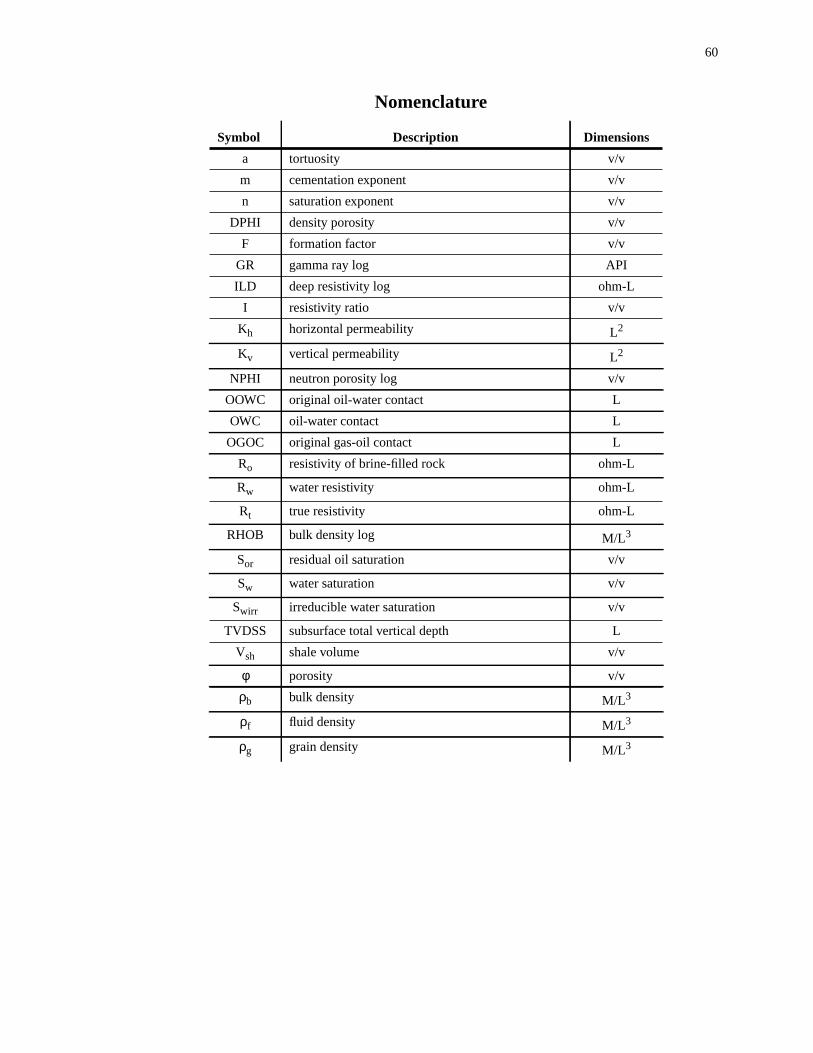
60

Nomenclature

Symbol Description Dimensions

a tortuosity v/v

m cementation exponent v/v

n saturation exponent v/v

DPHI density porosity v/v

F formation factor v/v

GR gamma ray log API

ILD deep resistivity log ohm-L

I resistivity ratio v/v

Kh horizontal permeability L2

Kv vertical permeability L2

NPHI neutron porosity log v/v

OOWC original oil-water contact L

OWC oil-water contact L

OGOC original gas-oil contact L

Ro resistivity of brine-filled rock ohm-L

Rw water resistivity ohm-L

Rt true resistivity ohm-L

RHOB bulk density log M/L3

Sor residual oil saturation v/v

Sw water saturation v/v

Swirr irreducible water saturation v/v

TVDSS subsurface total vertical depth L

Vsh shale volume v/v

φ porosity v/v

ρb bulk density M/L3

ρf fluid density M/L3

ρg grain density M/L3

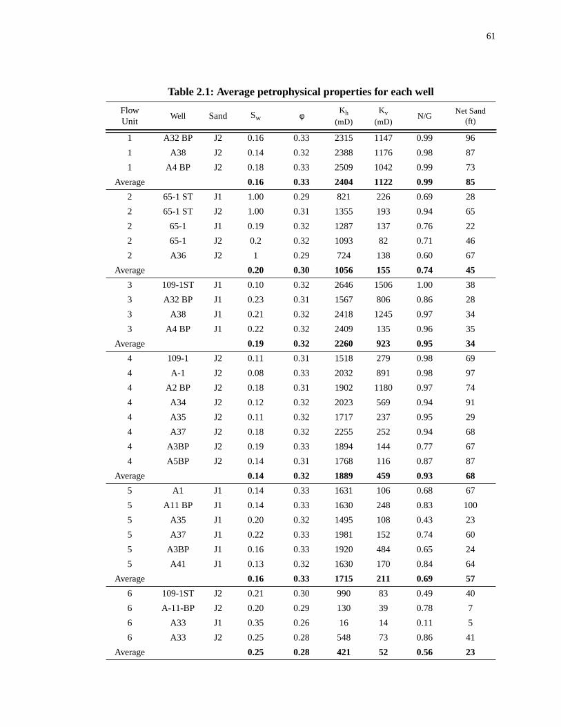
61

Table 2.1: Average petrophysical properties for each well

FlowUnit

Well Sand Sw φKh

(mD)

Kv

(mD)N/G

Net Sand(ft)

1 A32 BP J2 0.16 0.33 2315 1147 0.99 96

1 A38 J2 0.14 0.32 2388 1176 0.98 87

1 A4 BP J2 0.18 0.33 2509 1042 0.99 73

Average 0.16 0.33 2404 1122 0.99 85

2 65-1 ST J1 1.00 0.29 821 226 0.69 28

2 65-1 ST J2 1.00 0.31 1355 193 0.94 65

2 65-1 J1 0.19 0.32 1287 137 0.76 22

2 65-1 J2 0.2 0.32 1093 82 0.71 46

2 A36 J2 1 0.29 724 138 0.60 67

Average 0.20 0.30 1056 155 0.74 45

3 109-1ST J1 0.10 0.32 2646 1506 1.00 38

3 A32 BP J1 0.23 0.31 1567 806 0.86 28

3 A38 J1 0.21 0.32 2418 1245 0.97 34

3 A4 BP J1 0.22 0.32 2409 135 0.96 35

Average 0.19 0.32 2260 923 0.95 34

4 109-1 J2 0.11 0.31 1518 279 0.98 69

4 A-1 J2 0.08 0.33 2032 891 0.98 97

4 A2 BP J2 0.18 0.31 1902 1180 0.97 74

4 A34 J2 0.12 0.32 2023 569 0.94 91

4 A35 J2 0.11 0.32 1717 237 0.95 29

4 A37 J2 0.18 0.32 2255 252 0.94 68

4 A3BP J2 0.19 0.33 1894 144 0.77 67

4 A5BP J2 0.14 0.31 1768 116 0.87 87

Average 0.14 0.32 1889 459 0.93 68

5 A1 J1 0.14 0.33 1631 106 0.68 67

5 A11 BP J1 0.14 0.33 1630 248 0.83 100

5 A35 J1 0.20 0.32 1495 108 0.43 23

5 A37 J1 0.22 0.33 1981 152 0.74 60

5 A3BP J1 0.16 0.33 1920 484 0.65 24

5 A41 J1 0.13 0.32 1630 170 0.84 64

Average 0.16 0.33 1715 211 0.69 57

6 109-1ST J2 0.21 0.30 990 83 0.49 40

6 A-11-BP J2 0.20 0.29 130 39 0.78 7

6 A33 J1 0.35 0.26 16 14 0.11 5

6 A33 J2 0.25 0.28 548 73 0.86 41

Average 0.25 0.28 421 52 0.56 23

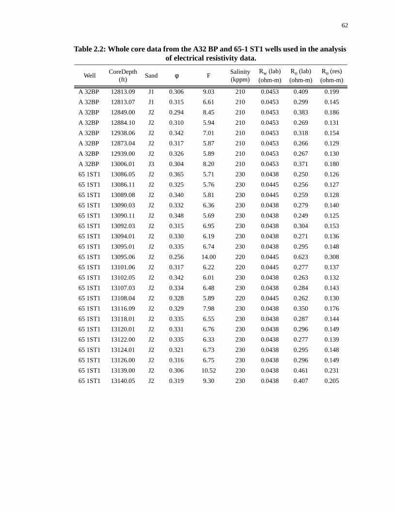
62

Table 2.2: Whole core data from the A32 BP and 65-1 ST1 wells used in the analysisof electrical resistivity data.

WellCoreDepth

(ft)Sand φ F

Salinity(kppm)

Rw (lab)(ohm-m)

Ro (lab)(ohm-m)

Ro (res)(ohm-m)

A 32BP 12813.09 J1 0.306 9.03 210 0.0453 0.409 0.199

A 32BP 12813.07 J1 0.315 6.61 210 0.0453 0.299 0.145

A 32BP 12849.00 J2 0.294 8.45 210 0.0453 0.383 0.186

A 32BP 12884.10 J2 0.310 5.94 210 0.0453 0.269 0.131

A 32BP 12938.06 J2 0.342 7.01 210 0.0453 0.318 0.154

A 32BP 12873.04 J2 0.317 5.87 210 0.0453 0.266 0.129

A 32BP 12939.00 J2 0.326 5.89 210 0.0453 0.267 0.130

A 32BP 13006.01 J3 0.304 8.20 210 0.0453 0.371 0.180

65 1ST1 13086.05 J2 0.365 5.71 230 0.0438 0.250 0.126

65 1ST1 13086.11 J2 0.325 5.76 230 0.0445 0.256 0.127

65 1ST1 13089.08 J2 0.340 5.81 230 0.0445 0.259 0.128

65 1ST1 13090.03 J2 0.332 6.36 230 0.0438 0.279 0.140

65 1ST1 13090.11 J2 0.348 5.69 230 0.0438 0.249 0.125

65 1ST1 13092.03 J2 0.315 6.95 230 0.0438 0.304 0.153

65 1ST1 13094.01 J2 0.330 6.19 230 0.0438 0.271 0.136

65 1ST1 13095.01 J2 0.335 6.74 230 0.0438 0.295 0.148

65 1ST1 13095.06 J2 0.256 14.00 220 0.0445 0.623 0.308

65 1ST1 13101.06 J2 0.317 6.22 220 0.0445 0.277 0.137

65 1ST1 13102.05 J2 0.342 6.01 230 0.0438 0.263 0.132

65 1ST1 13107.03 J2 0.334 6.48 230 0.0438 0.284 0.143

65 1ST1 13108.04 J2 0.328 5.89 220 0.0445 0.262 0.130

65 1ST1 13116.09 J2 0.329 7.98 230 0.0438 0.350 0.176

65 1ST1 13118.01 J2 0.335 6.55 230 0.0438 0.287 0.144

65 1ST1 13120.01 J2 0.331 6.76 230 0.0438 0.296 0.149

65 1ST1 13122.00 J2 0.335 6.33 230 0.0438 0.277 0.139

65 1ST1 13124.01 J2 0.321 6.73 230 0.0438 0.295 0.148

65 1ST1 13126.00 J2 0.316 6.75 230 0.0438 0.296 0.149

65 1ST1 13139.00 J2 0.306 10.52 230 0.0438 0.461 0.231

65 1ST1 13140.05 J2 0.319 9.30 230 0.0438 0.407 0.205

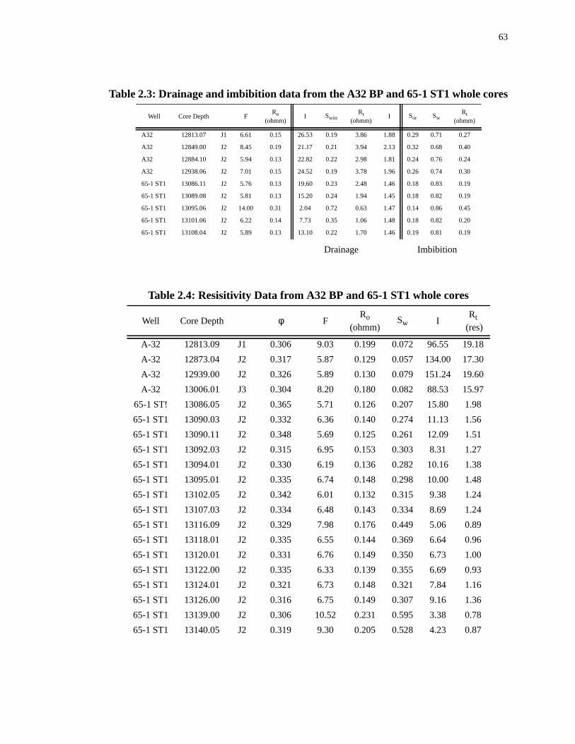
63

Drainage Imbibition

Table 2.3: Drainage and imbibition data from the A32 BP and 65-1 ST1 whole cores

Well Core Depth FRo

(ohmm)I Swirr

Rt(ohmm)

I Sor SwRt

(ohmm)

A32 12813.07 J1 6.61 0.15 26.53 0.19 3.86 1.88 0.29 0.71 0.27

A32 12849.00 J2 8.45 0.19 21.17 0.21 3.94 2.13 0.32 0.68 0.40

A32 12884.10 J2 5.94 0.13 22.82 0.22 2.98 1.81 0.24 0.76 0.24

A32 12938.06 J2 7.01 0.15 24.52 0.19 3.78 1.96 0.26 0.74 0.30

65-1 ST1 13086.11 J2 5.76 0.13 19.60 0.23 2.48 1.46 0.18 0.83 0.19

65-1 ST1 13089.08 J2 5.81 0.13 15.20 0.24 1.94 1.45 0.18 0.82 0.19

65-1 ST1 13095.06 J2 14.00 0.31 2.04 0.72 0.63 1.47 0.14 0.86 0.45

65-1 ST1 13101.06 J2 6.22 0.14 7.73 0.35 1.06 1.48 0.18 0.82 0.20

65-1 ST1 13108.04 J2 5.89 0.13 13.10 0.22 1.70 1.46 0.19 0.81 0.19

Table 2.4: Resisitivity Data from A32 BP and 65-1 ST1 whole cores

Well Core Depth φ FRo

(ohmm)Sw I

Rt

(res)

A-32 12813.09 J1 0.306 9.03 0.199 0.072 96.55 19.18

A-32 12873.04 J2 0.317 5.87 0.129 0.057 134.00 17.30

A-32 12939.00 J2 0.326 5.89 0.130 0.079 151.24 19.60

A-32 13006.01 J3 0.304 8.20 0.180 0.082 88.53 15.97

65-1 ST! 13086.05 J2 0.365 5.71 0.126 0.207 15.80 1.98

65-1 ST1 13090.03 J2 0.332 6.36 0.140 0.274 11.13 1.56

65-1 ST1 13090.11 J2 0.348 5.69 0.125 0.261 12.09 1.51

65-1 ST1 13092.03 J2 0.315 6.95 0.153 0.303 8.31 1.27

65-1 ST1 13094.01 J2 0.330 6.19 0.136 0.282 10.16 1.38

65-1 ST1 13095.01 J2 0.335 6.74 0.148 0.298 10.00 1.48

65-1 ST1 13102.05 J2 0.342 6.01 0.132 0.315 9.38 1.24

65-1 ST1 13107.03 J2 0.334 6.48 0.143 0.334 8.69 1.24

65-1 ST1 13116.09 J2 0.329 7.98 0.176 0.449 5.06 0.89

65-1 ST1 13118.01 J2 0.335 6.55 0.144 0.369 6.64 0.96

65-1 ST1 13120.01 J2 0.331 6.76 0.149 0.350 6.73 1.00

65-1 ST1 13122.00 J2 0.335 6.33 0.139 0.355 6.69 0.93

65-1 ST1 13124.01 J2 0.321 6.73 0.148 0.321 7.84 1.16

65-1 ST1 13126.00 J2 0.316 6.75 0.149 0.307 9.16 1.36

65-1 ST1 13139.00 J2 0.306 10.52 0.231 0.595 3.38 0.78

65-1 ST1 13140.05 J2 0.319 9.30 0.205 0.528 4.23 0.87

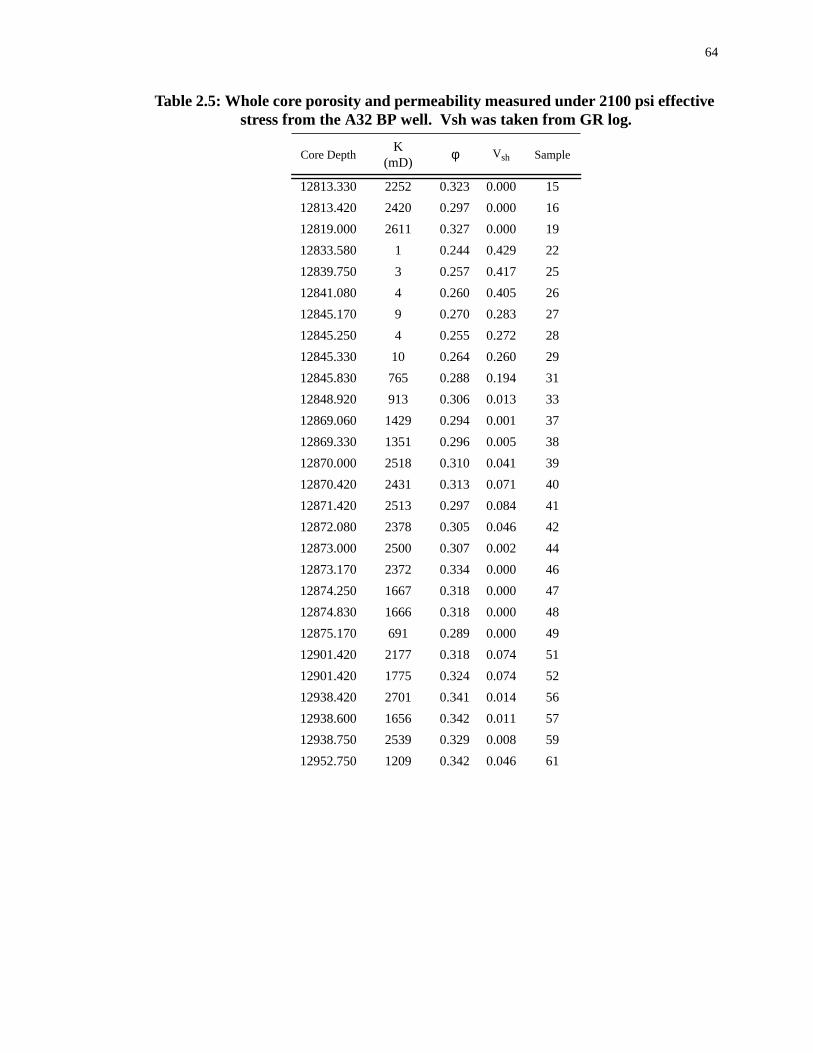
64

Table 2.5: Whole core porosity and permeability measured under 2100 psi effectivestress from the A32 BP well. Vsh was taken from GR log.

Core DepthK

(mD)φ Vsh Sample

12813.330 2252 0.323 0.000 15

12813.420 2420 0.297 0.000 16

12819.000 2611 0.327 0.000 19

12833.580 1 0.244 0.429 22

12839.750 3 0.257 0.417 25

12841.080 4 0.260 0.405 26

12845.170 9 0.270 0.283 27

12845.250 4 0.255 0.272 28

12845.330 10 0.264 0.260 29

12845.830 765 0.288 0.194 31

12848.920 913 0.306 0.013 33

12869.060 1429 0.294 0.001 37

12869.330 1351 0.296 0.005 38

12870.000 2518 0.310 0.041 39

12870.420 2431 0.313 0.071 40

12871.420 2513 0.297 0.084 41

12872.080 2378 0.305 0.046 42

12873.000 2500 0.307 0.002 44

12873.170 2372 0.334 0.000 46

12874.250 1667 0.318 0.000 47

12874.830 1666 0.318 0.000 48

12875.170 691 0.289 0.000 49

12901.420 2177 0.318 0.074 51

12901.420 1775 0.324 0.074 52

12938.420 2701 0.341 0.014 56

12938.600 1656 0.342 0.011 57

12938.750 2539 0.329 0.008 59

12952.750 1209 0.342 0.046 61

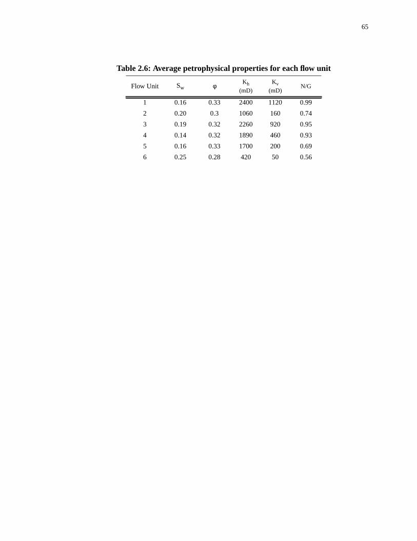
65

Table 2.6: Average petrophysical properties for each flow unit

Flow Unit Sw φKh

(mD)

Kv

(mD)N/G

1 0.16 0.33 2400 1120 0.99

2 0.20 0.3 1060 160 0.74

3 0.19 0.32 2260 920 0.95

4 0.14 0.32 1890 460 0.93

5 0.16 0.33 1700 200 0.69

6 0.25 0.28 420 50 0.56

66

es

ater

f the

was

l pro-

pro-

has

ction of

in

reas

ervoir

ic

Chapter 3

RESERVOIR MONITORING OF THE BULLWINKLE J SANDSUSING PRODUCTION DATA, PULSED NEUTRON LOGS, AND

GASSMANN FLUID SUBSTITUTION MODELING WITH COMPAR-ISON TO TIME-LAPSE SEISMIC RESULTS, GREEN CANYON

BLOCK 65, OFFSHORE LOUISIANA

Abstract

Hydrocarbon production from the J1 and J2 reservoirs resulted in dynamic chang

which are resolvable with time-lapse seismic data. Between 1989 and 1997, the oil-w

contact (OWC) had moved vertically by as much as 284 m. We track the movement o

OWC using production and pulsed neutron logs and we show that the position in 1997

not horizontal. The drainage scenario we develop from these data predict the actua

duced volumes within 8%. The seismic properties of the J1 and J2 were effected by

duction because of changes in effective stress and saturation. Time-lapse results

(Swanston et al., in review) show that the seismic amplitude in regions of water sweep

decreased. We use the Gassmann Equations to model the rock properties as a fun

effective stress and saturation. We found that water-swept areas exhibit an increase

acoustic impedance by as much as 30%. This 30% increase in acoustic impedance

resulted in a 70% decrease in the reflection coefficient at the top of the reservoirs. A

in the reservoir which have experienced an increase in gas saturation due to the res

pressure falling below the bubble point did not exhibit a noticeable change in acoust

impedance and reflection coefficient between 1989 and 1997.

67

s in

ges is

nd J2

ock

g

nd J2

1

ion

on-

2.

over

e

the

nced

d

ompac-

seis-

ith

in

pro-

Introduction

The J1 and J2 sands are a natural laboratory over which time-dependent change

saturation and seismic amplitude are studied. The driving force causing these chan

production of hydrocarbons from the J1 and J2 reservoirs. Production from the J1 a

sands began in July 1989 from the Bullwinkle Platform, located in Green Canyon Bl

65 in 412 m (1353 ft) of water. A total of 15 wells produced or are currently producin

from the J1 and J2 RB reservoirs. Of these 15, 4 wells produced from both the J1 a

in a commingled production string. Two wells, A1 and A38-ST, produced from the J

sand only. The remaining wells produced from the J2. In addition to the 15 product

wells, 5 water injection wells were drilled and perforated below the original oil-water c

tact (OOWC). Only one of the injection wells (A-9) is perforated in both the J1 and J

The remaining 4 wells inject into the J2 exclusively.

Time-lapse seismic analysis is the study of two or more seismic surveys acquired

the same area at different times. At Bullwinkle, two orthogonal seismic surveys wer

acquired prior to production in 1988. An additional seismic survey was acquired over

field in 1997, after 8 years of production. These surveys were normalized and differe

by Swanston et al. (in review) and show that it is possible to image production relate

changes in seismic response. These production related changes include reservoir c

tion and fluid contact movement.

The time-lapse analysis by Swanston et al. (in review) shows areas of widespread

mic dimming in places where oil has been drained from the J2 sand and replaced w

water. This chapter provides additional background to the work of Swanston et al. (

review) by tracking the movement of the oil-water contact (OWC) through time using

68

m

and

at

perfo-

they

ar-

ampli-

tic

d by

951)

ure.

c

mag-

urvey

n the

V

of the

of the

, that

duction data from individual wells and cased-hole wireline logs. Production data fro

individual wells record the amount of fluids (oil, water, and gas) extracted from the J1

J2 sands in terms of flow rate (barrels of fluid/day). We show that water production

each well increased when the OWC had moved updip to the same depth as the sand

rations in the well. Cased-hole wireline logs further aid in tracking the OWC because

can detect water in the formation while the well is still producing.

The acoustic properties of rocks dramatically change at Bullwinkle due to hydroc

bon production. Changes in saturation and effective stress will change the seismic

tude of the reservoir. This is because seismic amplitude is proportional to the acous

impedance contrast in the sand. The impedance behavior in turn is strongly affecte

the p-wave velocity (Vp) in the sand. We used the Gassmann Equations (Gassmann, 1

to model changes in Vp and impedance associated with changes in saturation and press

An increase in Sw and effective stress accompanied by a decrease in oil saturation

increases the velocity and acoustic impedance in the rock. This increase in acousti

impedance makes the reflection coefficient (RFC) at the top of the sand decrease in

nitude. The smaller RFC at the top of the sand was recorded in the second seismic s

in areas where oil had been drained from the J2 as a smaller amplitude.

Exsolution of gas during production has been shown to have the opposite effect o

seismic properties of a rock. While replacement of oil with water increases the Vp and

impedance, the presence of a free gas phase in the pore space dramatically reducesp and

impedance and increases the magnitude of the RFC. The increase in RFC at the top

sand should be imaged as a seismic brightening through time, where the magnitude

seismic amplitude in 1997 is greater than the amplitude in 1988. We show, however

69

s has

quired

inal

is

WC

con-

than

al

filled

WC

o des-

0 m,

aces

igh as

stiffening of the rock due to compaction is enough to cancel out the effect that free ga

on the acoustic properties.

Production Characterization

J1 and J2 Initial Volumes

Structure maps of the J1 and J2 sands were constructed using 3D seismic data ac

before production began at Bullwinkle in 1988 (Swanston et al., in review). The orig

oil-water contact (OOWC) was imaged with seismic data and its subsurface position

supported by well penetrations in both the reservoir and aquifer of each sand. The OO

in both sands is delineated by a sharp break in seismic amplitude along a structural

tour. The magnitude of the seismic amplitude in the reservoir is 5 to 10 times greater

in the aquifer. The OOWC was placed at 3,755 m (12,320 ft) subsurface total vertic

depth (TVDSS) in the J1 and 3,784 m (12,415 ft) TVDSS in the J2.

Net pay within the J1 and J2 is defined as the vertical thickness of hydrocarbon-

sand and it is derived from well log measurements. There is 0 m of net pay at the OO

(Figures 3.1 and 3.2) . The outline which defines the areal extent of each sand is als

ignated with 0 m net pay (Figures 3.1 and 3.2). Net pay in the J2 ranges from 0 to 3

with maximum values near the A34 and A1 wells (Figure 3.1). The J1 sand in most pl

is not as thick as the J2, although net pay in the vicinity of the A11 BP reaches as h

30 m (Figure 3.2).

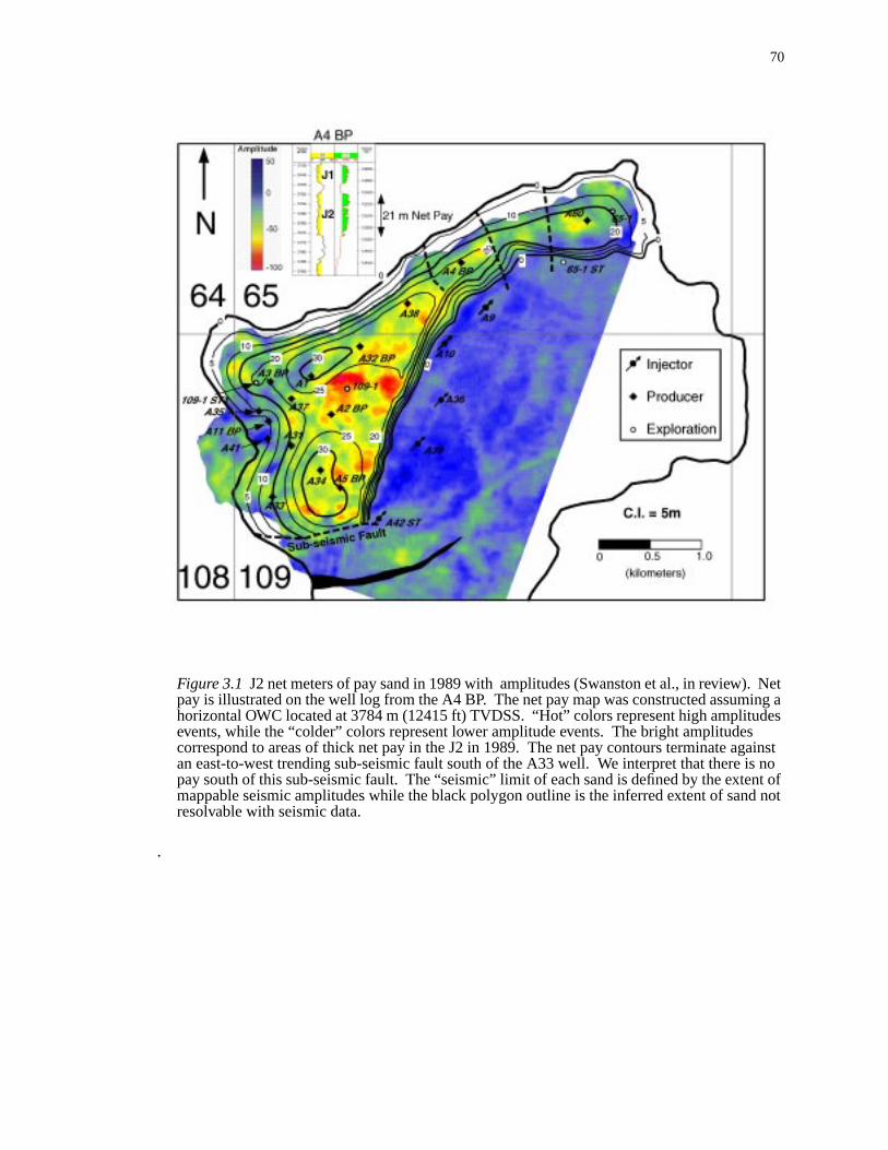
70

Neting adessgainstis not of

d not

Figure 3.1 J2 net meters of pay sand in 1989 with amplitudes (Swanston et al., in review).pay is illustrated on the well log from the A4 BP. The net pay map was constructed assumhorizontal OWC located at 3784 m (12415 ft) TVDSS. “Hot” colors represent high amplituevents, while the “colder” colors represent lower amplitude events. The bright amplitudecorrespond to areas of thick net pay in the J2 in 1989. The net pay contours terminate aan east-to-west trending sub-seismic fault south of the A33 well. We interpret that there pay south of this sub-seismic fault. The “seismic” limit of each sand is defined by the extenmappable seismic amplitudes while the black polygon outline is the inferred extent of sanresolvable with seismic data.

.

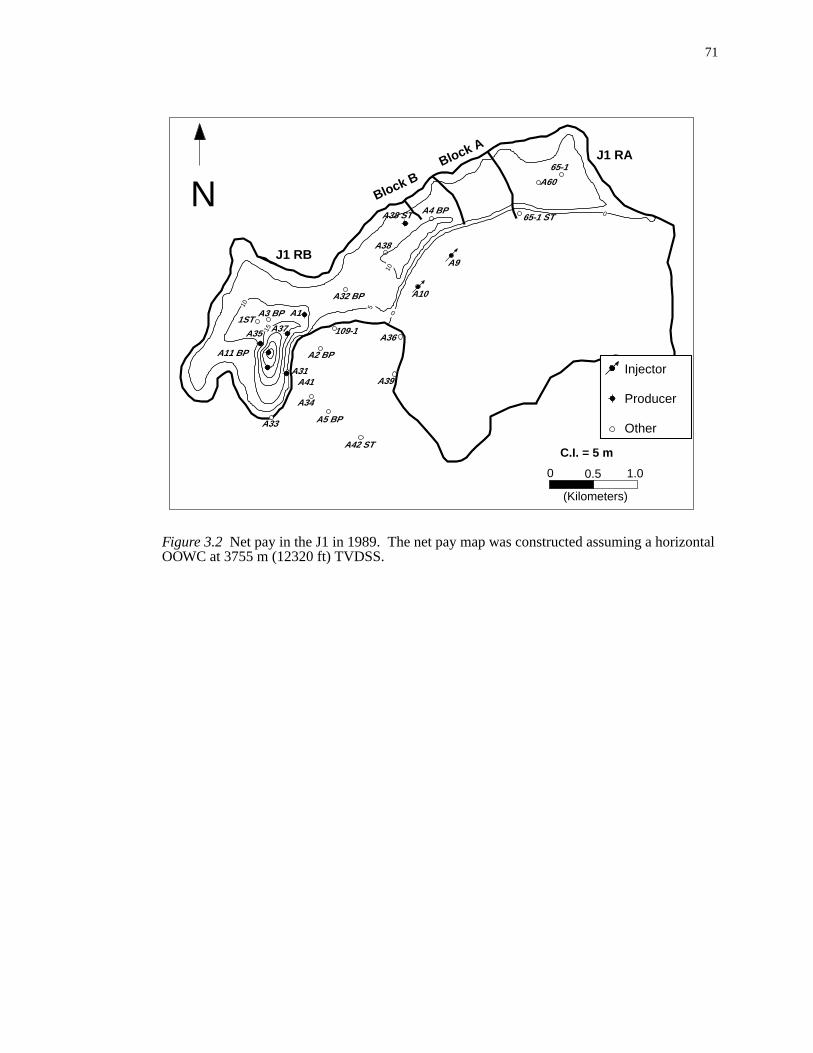
71

ontal
Figure 3.2 Net pay in the J1 in 1989. The net pay map was constructed assuming a horizOOWC at 3755 m (12320 ft) TVDSS.
A31

A33

A32 BP

A38

A4 BP65-1 ST

A60

65-1

A35

A3 BP A1

A41

0 0.5 1.0

(Kilometers)

N

A5 BP

109-1

A2 BP

C.I. = 5 m

A34

A11 BP

1ST

A42 ST

A39

A36

A10

A9

A38 ST

A37

Injector

Producer

Other

0

0

5

10

15

J1 RABlock A

Block B

J1 RB10

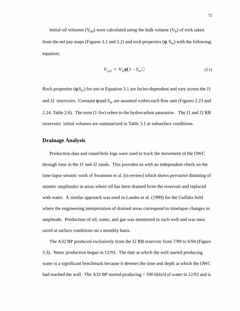
72

e J1

d

2 RB

C

n the

g of

ced

ges in

ea-

ure

g

OWC

nd is

Initial oil volumes (Voil) were calculated using the bulk volume (Vb) of rock taken

from the net pay maps (Figures 3.1 and 3.2) and rock properties (φ, Sw) with the following

equation:

. (3.1)

Rock properties (φ,Sw) for use in Equation 3.1 are facies-dependent and vary across th

and J2 reservoirs. Constantφ and Sw are assumed within each flow unit (Figures 2.23 an

2.24, Table 2.6). The term (1-Sw) refers to the hydrocarbon saturation . The J1 and J

reservoirs initial volumes are summarized in Table 3.1 at subsurface conditions.

Drainage Analysis

Production data and cased-hole logs were used to track the movement of the OW

through time in the J1 and J2 sands. This provides us with an independent check o

time-lapse seismic work of Swanston et al. (in review) which shows pervasive dimmin

seismic amplitudes in areas where oil has been drained from the reservoir and repla

with water. A similar approach was used in Landro et al. (1999) for the Gulfaks field

where the engineering interpretation of drained areas correspond to timelapse chan

amplitude. Production of oil, water, and gas was monitored in each well and was m

sured at surface conditions on a monthly basis.

The A32 BP produced exclusively from the J2 RB reservoir from 7/89 to 6/94 (Fig

3.3). Water production began in 12/93. The date at which the well started producin

water is a significant benchmark because it denotes the time and depth at which the

had reached the well. The A32 BP started producing > 100 bbls/d of water in 12/93 a

Voil Vbφ 1 Sw–( )=

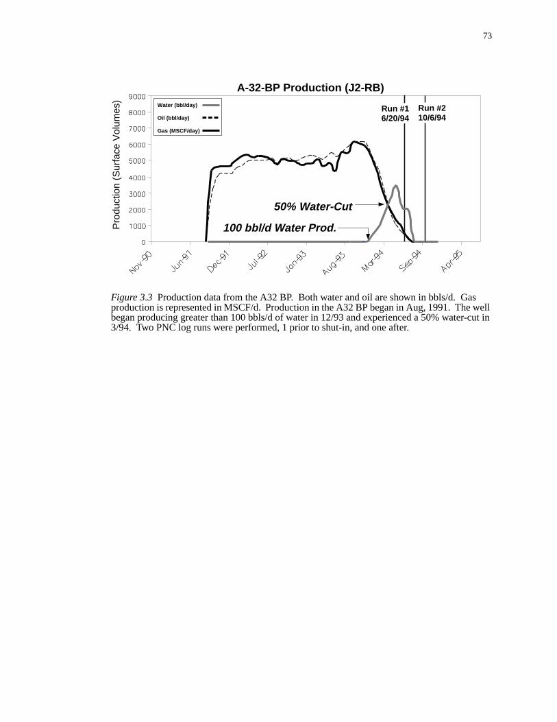
73

swellcut in

Figure 3.3 Production data from the A32 BP. Both water and oil are shown in bbls/d. Gaproduction is represented in MSCF/d. Production in the A32 BP began in Aug, 1991. Thebegan producing greater than 100 bbls/d of water in 12/93 and experienced a 50% water-3/94. Two PNC log runs were performed, 1 prior to shut-in, and one after.

A-32-BP Production (J2-RB)

Pro

duct

ion

(Sur

face

Vol

umes

)Run #16/20/94

Run #210/6/94

Water (bbl/day)

Oil (bbl/day)

Gas (MSCF/day)

50% Water-Cut

100 bbl/d Water Prod.

74

on

phi-

acteris-

ue

g after

ogs

e J1

at

ows

uration

inter-

J1

il satu-

ction

3.6

blue

per-

er ear-

h

denoted as the “significant water-cut”. The point at which the volumetric oil producti

rate is equal to the water production rate is called the “50% water-cut”. Figure 3.4 gra

cally illustrates the production timescales for the well data in Table 3.2.

Pulsed neutron capture (PNC) logs were also used to investigate drainage char

tics and to track the movement of the oil-water contact (OWC). These logs are uniq

because they can detect the presence of hydrocarbons in the formation behind casin

the well has been producing. Additional information concerning the theory of PNC l

and their use in interpretation is found in Appendix A.

The openhole logs acquired when the A32 BP was drilled in 2/91 show that both th

and J2 are initially oil-filled (Figure 3.5). The PNC run in 6/94 for the A32 BP shows th

the J1 was still oil-filled and the J2 had been water swept. The PNC run in 10/94 sh

that the J1 had been water-swept and the J2 experienced a slight increase in oil-sat

at the top of the sand. This increase in oil saturation at the top of the J2 in 10/94 is

preted to result from bypassed oil migrating upstructure. The remaining oil left in the

and J2 sands after the last PNC log run in 1994 is given a specific name: residual o

ration (Sor). For the A32 BP, Sor is variable and ranges from 0.20 to 0.50 (Figure 3.5).

We compared the depths and times at which wells began significant water produ

(> 100 bbls/d) to PNC log interpretations (Figure 3.6). The solid back lines in Figure

represent the time and depth interval over which a well began producing water. The

and green lines represent the time and depth interval over which PNC log runs were

formed. In general, we observed that wells lower on structure began producing wat

lier than wells located farther updip. The PNC interpretations show that sands whic

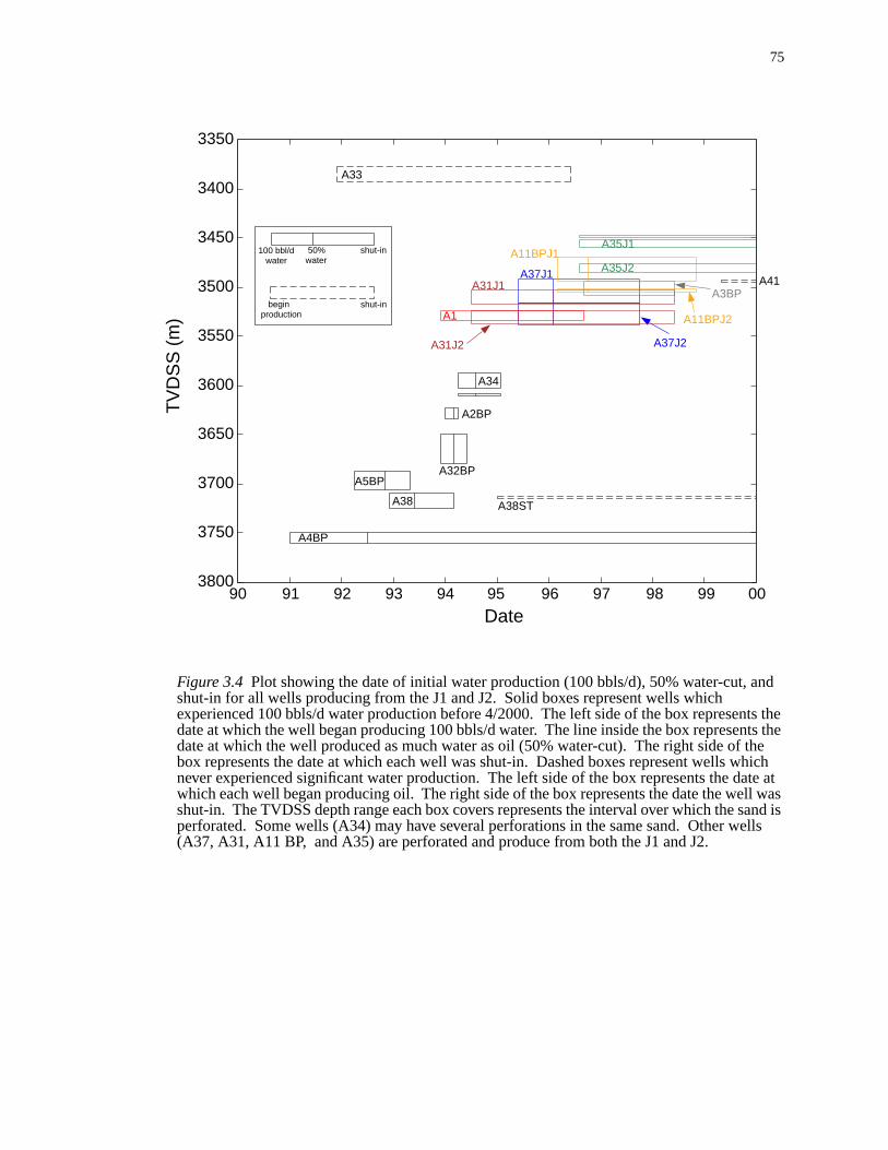
75

nd

ts thets thethehich

ate atl wasand isells

Figure 3.4 Plot showing the date of initial water production (100 bbls/d), 50% water-cut, ashut-in for all wells producing from the J1 and J2. Solid boxes represent wells whichexperienced 100 bbls/d water production before 4/2000. The left side of the box represendate at which the well began producing 100 bbls/d water. The line inside the box represendate at which the well produced as much water as oil (50% water-cut). The right side of box represents the date at which each well was shut-in. Dashed boxes represent wells wnever experienced significant water production. The left side of the box represents the dwhich each well began producing oil. The right side of the box represents the date the welshut-in. The TVDSS depth range each box covers represents the interval over which the sperforated. Some wells (A34) may have several perforations in the same sand. Other w(A37, A31, A11 BP, and A35) are perforated and produce from both the J1 and J2.

3350

3400

3450

3500

3550

3600

3650

3700

3750

3800

A1

A2BP

A4BP

A5BPA32BP

A38

A34

A11BPJ1

A31J1

A31J2

A37J1 A35J2

A35J1

A3BP

A38ST

A41

A33

A11BPJ2

A37J2

90 91 92 93 94 95 96 97 98 99 00

TV

DS

S (

m)

Date

100 bbl/d water

50%water

shut-in

begin production

shut-in

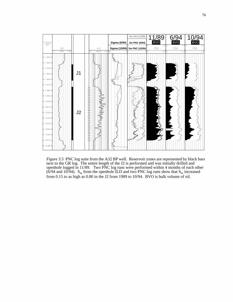
76

bars

ther

Figure 3.5 PNC log suite from the A32 BP well. Reservoir zones are represented by blacknext to the GR log. The entire length of the J2 is perforated and was initially drilled andopenhole logged in 11/89. Two PNC log runs were performed within 4 months of each o(6/94 and 10/94). Sw from the openhole ILD and two PNC log runs show that Sw increasedfrom 0.15 to as high as 0.80 in the J2 from 1989 to 10/94. BVO is bulk volume of oil.

Sw PNC (10/94)

Sw PNC (6/94)

Sw OH (11/89)

Sigma (6/94)

Sigma (10/94)

BVO BVO BVO11/89 6/94 10/94

J1

J2

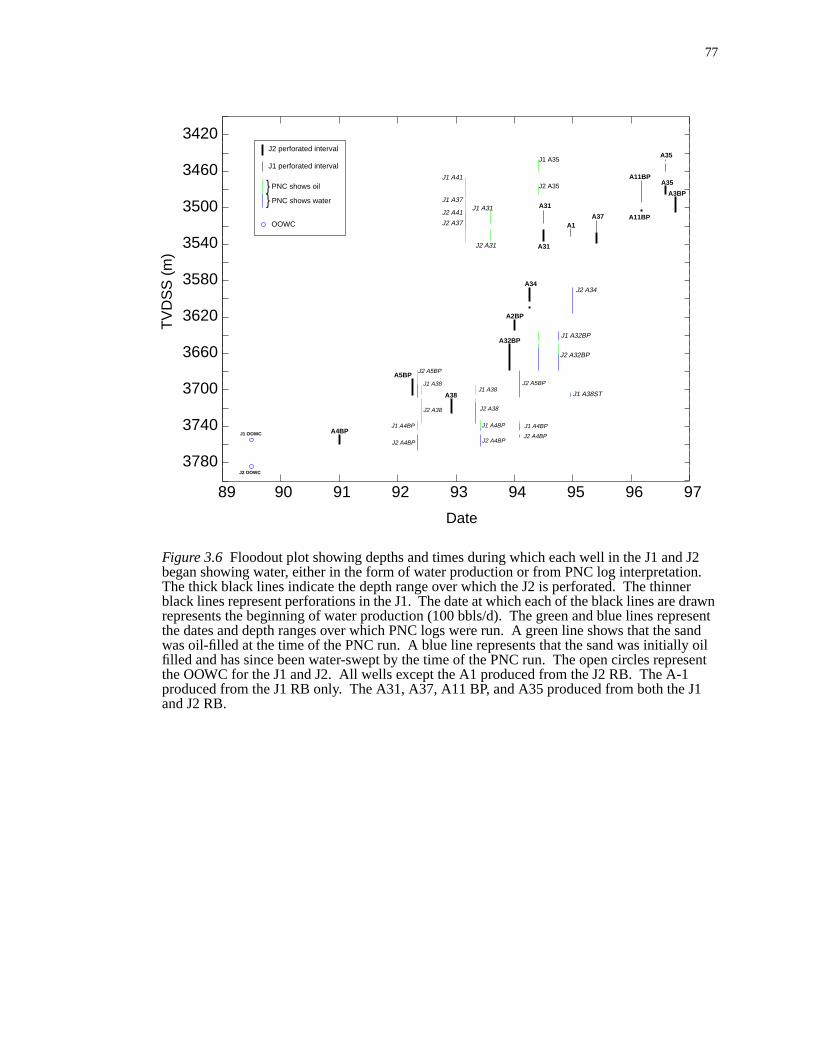
77

J2n.

errawn

resentsand oilesent

J1

Figure 3.6 Floodout plot showing depths and times during which each well in the J1 and began showing water, either in the form of water production or from PNC log interpretatioThe thick black lines indicate the depth range over which the J2 is perforated. The thinnblack lines represent perforations in the J1. The date at which each of the black lines are drepresents the beginning of water production (100 bbls/d). The green and blue lines repthe dates and depth ranges over which PNC logs were run. A green line shows that the was oil-filled at the time of the PNC run. A blue line represents that the sand was initiallyfilled and has since been water-swept by the time of the PNC run. The open circles reprthe OOWC for the J1 and J2. All wells except the A1 produced from the J2 RB. The A-1produced from the J1 RB only. The A31, A37, A11 BP, and A35 produced from both theand J2 RB.

89 90 91 92 93 94 95 96 97

3420

3460

3500

3540

3580

3620

3660

3700

3740

3780

A35

A35

A1

A2BP

A4BP

A5BP

A38

A32BP

A34

A11BP

A31

A37

J1 A32BP

J2 A32BP

J2 A34

J1 A41

J2 A41J1 A31

J2 A31

J1 A4BP

J2 A4BP

J1 A4BP

J2 A4BP

J1 A4BP

J2 A4BP

J1 A37

J2 A37

J2 A5BP

J2 A5BP

J1 A35

J2 A35

J1 A38

J2 A38

J1 A38

J2 A38

J1 A38ST

A31

A3BP

A11BP

J1 OOWC

J2 OOWC

J2 perforated interval

J1 perforated interval

PNC shows oil

PNC shows water}}

OOWC

TV

DS

S (

m)

Date

78

1,

well

P.

ion

m

ince

ure

/92

S

he

ntil

een

aced

s the

ure

were completely oil-filled were not producing water at the time of the logging run (A4

A37, A31, A35 in Figure 3.6). PNC logs imaged water-swept sands after a particular

began producing water (A5 BP, A38, A32 BP, A34, A4 BP in Figure 3.6).

OWC Movement: 1989-1992

Initial hydrocarbon production in the J2 RB reservoir began in 7/89 with the A4 B

The A2 BP began producing from the J2 RB 1 month later, followed by initial product

in the J1 RB from the A-1 well in 9/89. The first significant water production came fro

the A4 BP in 1/91 (Figure 3.6). In the vicinity of the A4 BP well, we show that the

OOWC had moved upwards 24 m to 3760 m TVDSS by 1/91 in the J2 (Figure 3.7). S

we only have one datum point, we assume that this contact was horizontal.


By 1993, there is sufficient data to interpret that the OWC was is not horizontal (Fig

3.7). Water production began in the southern portion of the J2 RB with the A5 BP in 4

(Figure 3.6) . A PNC log run in 5/92 in the A5 BP imaged an OWC at 3694 m TVDS

(Figure 3.6). However, a PNC log run in 5/92 still showed oil downdip of the A5 BP in t

J2 and J1 of the A38. In fact, the A38 did not begin water production from the J2 RB u

12/92. Downdip of the A38, a PNC run in the A4 B in 5/92 indicated that the J2 had b

completely water-swept and that the J1 was still oil-filled. Based on these data, we pl

the OWC in 1993 at the top of the J2 perforations in the area of the A4 BP. This wa

highest level water reached in the compartment just above the A4 BP (Block B in Fig

3.7). The OWC in the vicinity of the A38 in 1993 was placed at the bottom of the

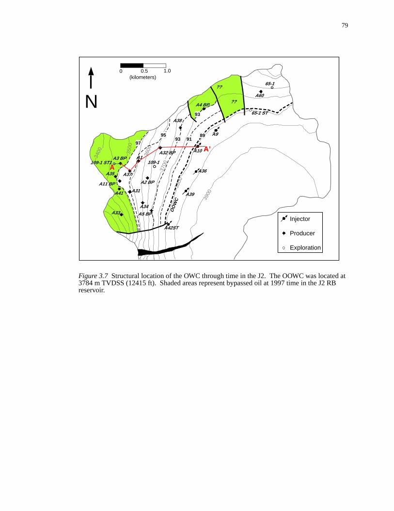
79

d atRB

Figure 3.7 Structural location of the OWC through time in the J2. The OOWC was locate3784 m TVDSS (12415 ft). Shaded areas represent bypassed oil at 1997 time in the J2 reservoir.

3900

3800

3700

3600

3500

3400

N

109-1 ST1A1

A35

A11 BP

A41

A33A34

A37

A5 BP

A36

A3 BP109-1

A32 BP

A2 BP

A38

A10

A4 BP

65-1 ST

A60

65-1

A9

OO

WC

Injector

Producer

Exploration

0 0.5 1.0(kilometers)

899193

95

97

??

??

93

A42ST

A39A31

A

A’

80

1993

no

ve-

C log

n in

n the

,

SS in

7).

e end

sed

2

(Fig-

l had

ion as

perforations (3720 m TVDSS). In the southern portion of the J2 RB, we placed the

OWC within the upper portion of the A5 BP perforations (3690 m TVDSS). There are

data to constrain a 1993 OWC in the J1, however, we still interpret some vertical mo

ment (Figure 3.8).


First signs of water movement in the J1 RB at the A4 BP was recorded by a PN

run in 6/93 (Figures 3.6 and 3.8). Also in 6/93, water was imaged with a PNC log ru

the A38 J2 RB just as it reached its 50% water-cut in 6/93. Updip, the A31 and A37

started producing from both the J1 and J2. PNC log runs were also performed updip i

A41, A37 and A31, all of which imaged oil in both the J1 and J2. By the end of 1993

water production began in the A32 BP and A2 BP from the J2.


Water encroachment by the end of 1995 in the J2 reached as high as 3540 m TVD

the vicinity of the A31 well which began water production in 7/94. (Figures 3.6 and 3.

The OWC above the A32 BP, however, was interpreted to lie at 3650 m. Other wells

updip of the A32 BP had also begun water production, or had even been shut-in by th

of 1995 (A2 BP and A34 in Figure 3.6).

We interpret the non-horizontal behavior of the OWC in the J2 to result from bypas

oil downdip of the A32 BP migrating up structure. The PNC log run in 6/94 in the A3

BP showed that the J2 was almost completely water-swept and the J1 was oil filled

ures 3.5 and 3.6). However, the A32 BP was PNC logged again in 10/94 after the wel

been shut-in and showed that water had swept completely through the J1. Oil saturat

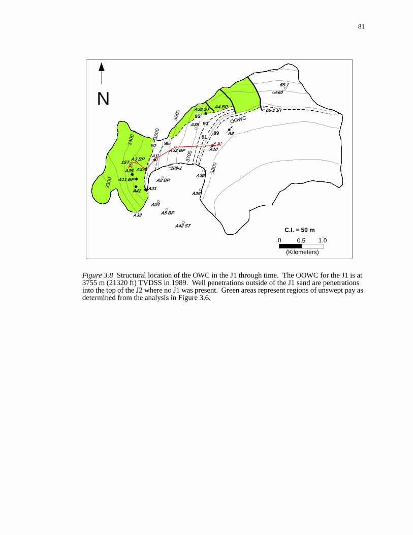
81

s attionspay as

Figure 3.8 Structural location of the OWC in the J1 through time. The OOWC for the J1 i3755 m (21320 ft) TVDSS in 1989. Well penetrations outside of the J1 sand are penetrainto the top of the J2 where no J1 was present. Green areas represent regions of unsweptdetermined from the analysis in Figure 3.6.

A31

A33

A32 BP

A38

A4 BP65-1 ST

A60

65-1

A35

A3 BPA1

A41

0 0.5 1.0

(Kilometers)

N

A5 BP

109-1

A2 BP

C.I. = 50 m

A34

A11 BP

1ST

A42 ST

A39

A36

A10

A9

3500

3600

3700

3800

3400

3300

OOWC

A38 ST

A37

89

9597

95

A

A’91

93

82

th the

cing

of

ntly

lat-

he

cing

A3

ny

on.

P,

P to

ns

imaged by the PNC log in the J2 sand of the A32 BP shows an increase compared wi

run in 6/94. We interpret this reintroduction of oil into the A32 BP area to result from

trapped oil just above the now shut-in A38 migrating upstructure.

OWC Movement: 1995 to 1996

We have two very good constraints for the J1 1995 OWC. The A-1 started produ

water in 1/95 (Figure 3.6). At that same time, the A38 ST1 was drilled 175 m downdip

the A1 and imaged an OWC at 3700 m TVDSS (Figure 3.8) . This well was subseque

perforated in the top 1m of the J1 and it produced oil with very little water through our

est production report in 4/2000.

There was very little vertical movement of the OWC from 1995 to 1996 in the J2. T

only new developments in terms of water occured at the A37, where it started produ

water from the J2 in 6/95 (Figure 3.6).


The updip region of the J2 began producing water during 1996 (A11 BP, A35, and

BP in Figure 3.6). The A33 had been producing from the J2 through 1996 without a

water. That well sanded up in 6/96, still without any signs of significant water producti

We placed the J2 1997 OWC close to 3500 m TVDSS in the vicinity of the A35, A11 B

and A41. The J2 1997 OWC reaches down to 3550 m TVDSS northeast of the A3 B

reflect the late movement of the downdip oil seen in 1994 and 1995.

The 1997 OWC in the J1 is at the same depth as the J2 OWC, with slight variatio

seen near the A37 and A31 wells.

83

s into

of

l

re

ough

) to

of

do

t the

both

areas.

d 3.8

ove

nes.

the

0).

cal-

ical

General OWC Behavior

The drainage analysis presented in Figures 3.7 and 3.8 provides several insight

the dynamic behavior of the OWC through time in the J1 and J2 sands. Production

hydrocarbons and water influx from the underlying aquifer has resulted in the vertica

movement of the OWC by 284 m (932 ft) in the J2 and 255 m (837 ft) in the J1 (Figu

3.9). Initially, the OOWC in the J1 and J2 were not located at the same depth, even th

both sands are connected in the reservoir. This behavior is explained by Best (2002

result from perched water present in the J1 not being displaced during the charging

both sands. Movement of the OWC from 1989 through 1992 in the J1 and J2 initially

not track each other (Figure3.9). By 1993, the OWCs for both sands were located a

same depth (3720 m). We interpret that the OWC equilibrated to the same depth in

sands by 1993 because they are hydraulically connected above the aquifer in some

J1 and J2 Volumes, 1997

J1 and J2 net pay maps were constructed using the 1997 OWC in Figures 3.7 an

(Figures 3.10 and 3.). Net pay in Figure 3.10 shows the amount of oil-filled sand ab

the 1997 OWC and does not take into account the oil left behind in the water-swept zo

Net pay within the J1 in 1997 ranged from 0 to 30 m, with the thickest area of pay in

A11 BP area (Figure 3.11). Net pay within the J2 ranged from 0 to 20 m (Figure 3.1

The bulk volumes of reservoir rock and oil in place above the OWC in 1997 were

culated using the net pay maps in Figures 3.10 and 3.11 and the flow unit petrophys

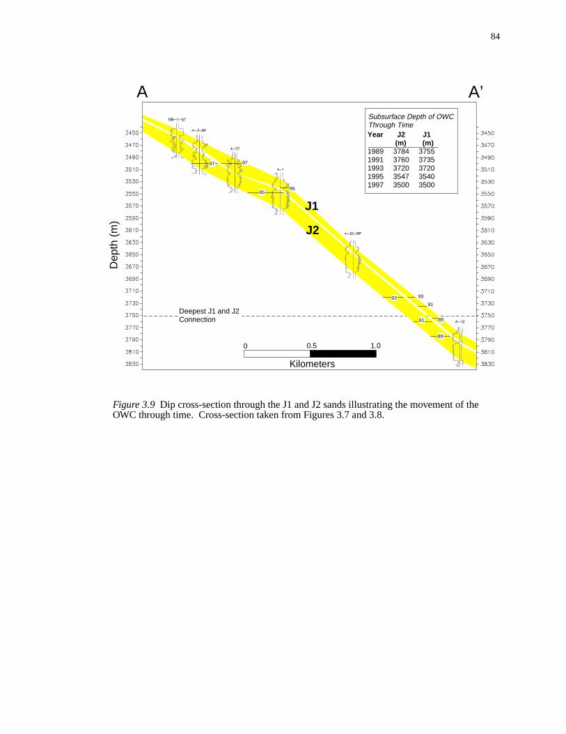
84

Figure 3.9 Dip cross-section through the J1 and J2 sands illustrating the movement of theOWC through time. Cross-section taken from Figures 3.7 and 3.8.

89

8991

93

97

91

93

95

Dep

th (

m)

0 0.5 1.0

Kilometers

A A’

95

97

Year J2 J1 (m) (m)

1989 3784 37551991 3760 37351993 3720 37201995 3547 35401997 3500 3500

Subsurface Depth of OWCThrough Time

J1

J2

Deepest J1 and J2 Connection

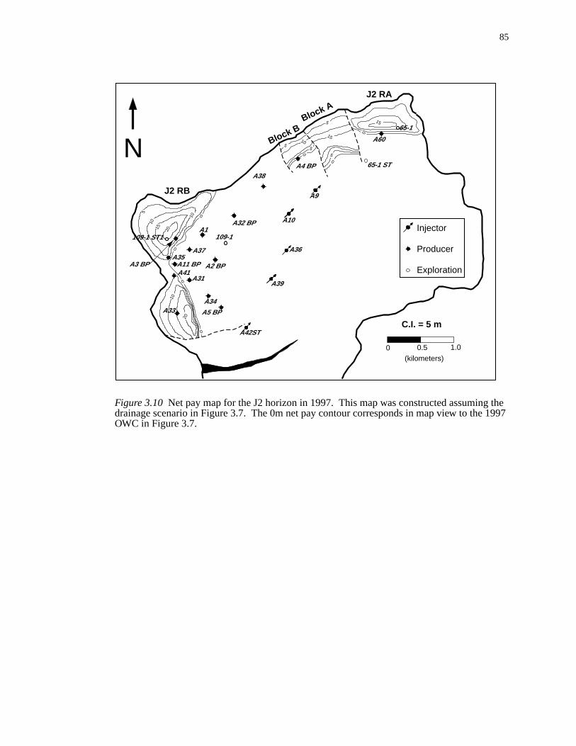
85

the 1997

Figure 3.10 Net pay map for the J2 horizon in 1997. This map was constructed assumingdrainage scenario in Figure 3.7. The 0m net pay contour corresponds in map view to theOWC in Figure 3.7.

N

109-1 ST1A1

A35A11 BPA41

A33A34

A37

A5 BP

A36

A3 BP

109-1

A32 BP

A2 BP

A38

A10

A4 BP 65-1 ST

A60

65-1

A9

Injector

Producer

Exploration

0 0.5 1.0

(kilometers)

A42ST

A39A31

0

0

0

010

1020

5

1015

20

0

5

105

5

5

15

0

0

15

C.I. = 5 m

J2 RA

Block A

Block B

J2 RB

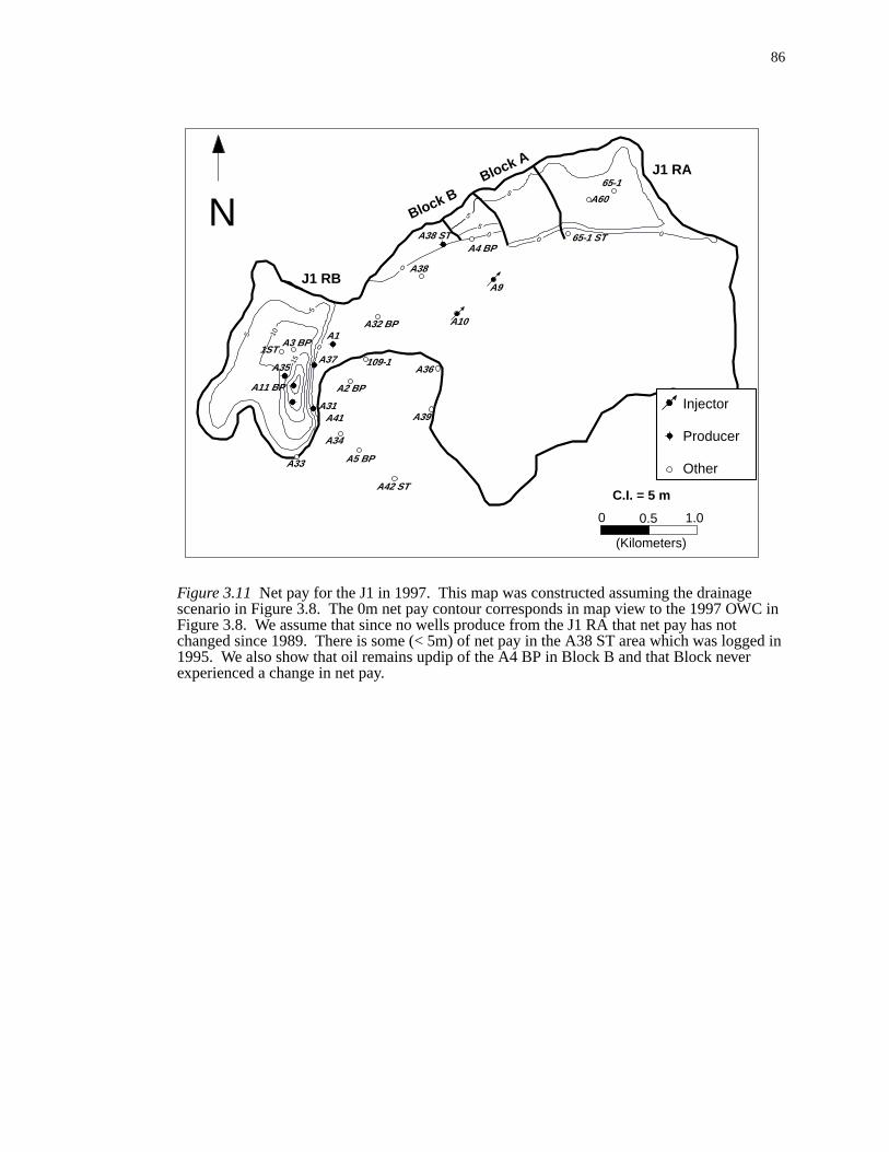
86

eC in

ed in

Figure 3.11 Net pay for the J1 in 1997. This map was constructed assuming the drainagscenario in Figure 3.8. The 0m net pay contour corresponds in map view to the 1997 OWFigure 3.8. We assume that since no wells produce from the J1 RA that net pay has notchanged since 1989. There is some (< 5m) of net pay in the A38 ST area which was logg1995. We also show that oil remains updip of the A4 BP in Block B and that Block neverexperienced a change in net pay.

A31

A33

A32 BP

A38

A4 BP65-1 ST

A60

65-1

A35

A3 BPA1

A41

0 0.5 1.0

(Kilometers)

N

A5 BP

109-1

A2 BP

C.I. = 5 m

A34

A11 BP

1ST

A42 ST

A39

A36

A10

A9

A38 ST

A37

Injector

Producer

Other

J1 RABlock A

Block B

J1 RB10

15

5

5

0

00

05

5

5

0

87

nd

f

3.14)

the

ickest

igure

a in

igure

d in

een

9 is

ining

eser-

for

en

properties (φ and 1-Sw) of Figures 2.23 and 2.24 and Table 2.6. Volumes of reservoir a

recoverable oil in 1997 for the J1 and J2 are summarized in Table 3.1.

Drained Pay Volumes for J1 and J2

A drained pay map shows the vertical thickness of sand that has been drained o

hydrocarbons (Figure 3.12). Drained pay maps for the J1 and J2 (Figures 3.13 and

were constructed by subtracting the 1997 net pay maps (Figures 3.10 and 3.11) from

1988 net pay maps (Figures 3.1 and 3.2). The J2 drained pay map shows that the th

areas of drained pay correspond to areas of intense seismic dimming (blue colors in F

3.13). Although movement of water was recorded from well logs and production dat

the J1, areas of drained pay do not correspond as well to areas of seismic dimming (F

3.14).

The ultimate goal in this drainage analysis is to compute from the maps presente

Figures 3.13 and 3.14 the volume of oil drained from the J1 and J2 reservoirs betw

1989 and 1997. This is accomplished by considering that the total volume of oil in 198

broken into 3 separate volumes:

(1) Volume of oil in place above the 1997 contact(2) Volume of non-recoverable oil remaining in place below the 1997 contact(3) Volume of oil recovered between 1989 and 1997

The bulk volume of reservoir which has been water-swept was calculated using the

drained pay maps in Figures 3.13 and 3.14. The volume of non-recoverable oil rema

in place below the 1997 OWC was calculated from the bulk volume of water-swept r

voir assuming a residual oil saturation (Sor of 0.25) and flow unit-dependent values

porosity (Figures 2.23 and 2.24 and Table 2.6). The volume of recovered oil was th

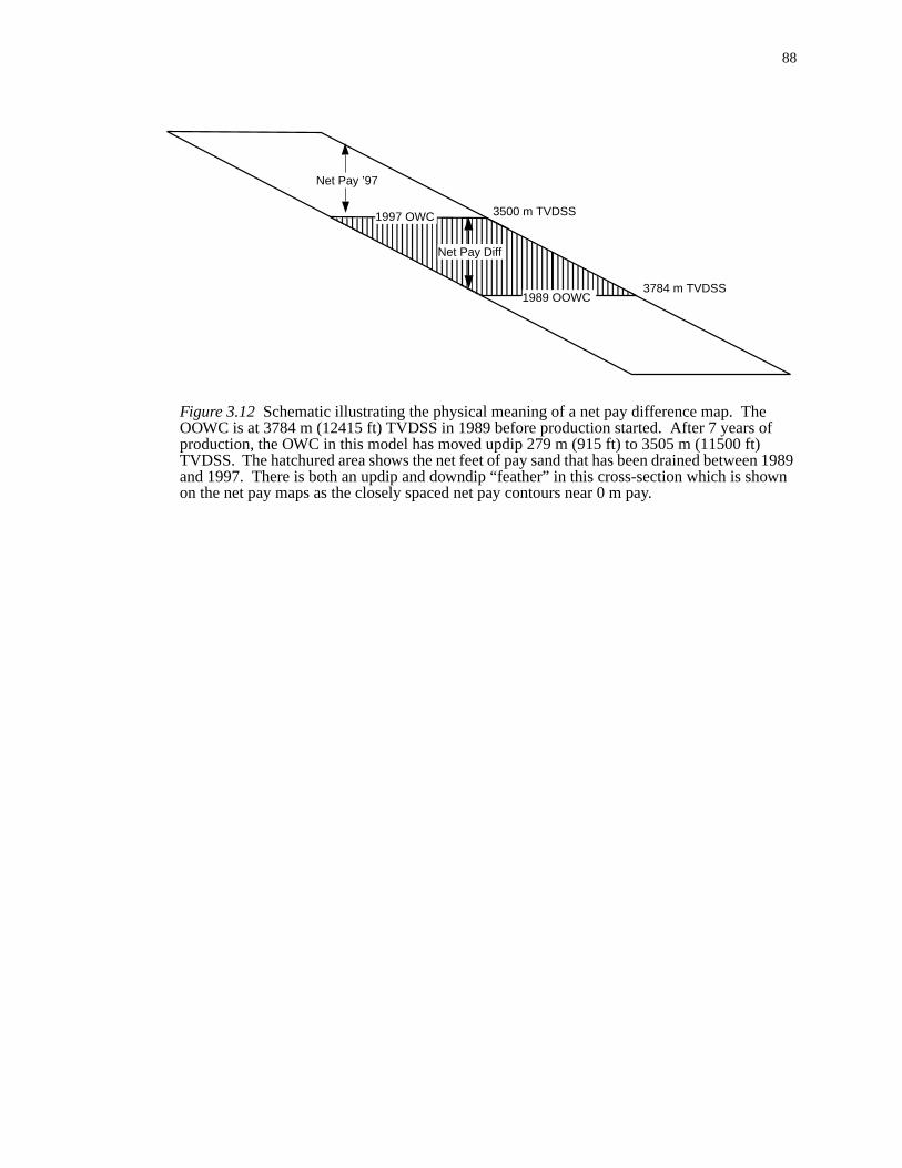
88

f

n 1989own

Figure 3.12 Schematic illustrating the physical meaning of a net pay difference map. TheOOWC is at 3784 m (12415 ft) TVDSS in 1989 before production started. After 7 years oproduction, the OWC in this model has moved updip 279 m (915 ft) to 3505 m (11500 ft)TVDSS. The hatchured area shows the net feet of pay sand that has been drained betweeand 1997. There is both an updip and downdip “feather” in this cross-section which is shon the net pay maps as the closely spaced net pay contours near 0 m pay.

3784 m TVDSS

3500 m TVDSS

1989 OOWC

1997 OWC

Net Pay Diff

Net Pay ’97

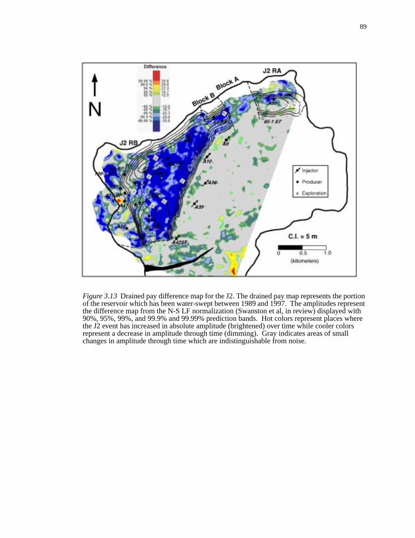
89

rtionresentith

wherers

ll

Figure 3.13 Drained pay difference map for the J2. The drained pay map represents the poof the reservoir which has been water-swept between 1989 and 1997. The amplitudes repthe difference map from the N-S LF normalization (Swanston et al, in review) displayed w90%, 95%, 99%, and 99.9% and 99.99% prediction bands. Hot colors represent places the J2 event has increased in absolute amplitude (brightened) over time while cooler colorepresent a decrease in amplitude through time (dimming). Gray indicates areas of smachanges in amplitude through time which are indistinguishable from noise.

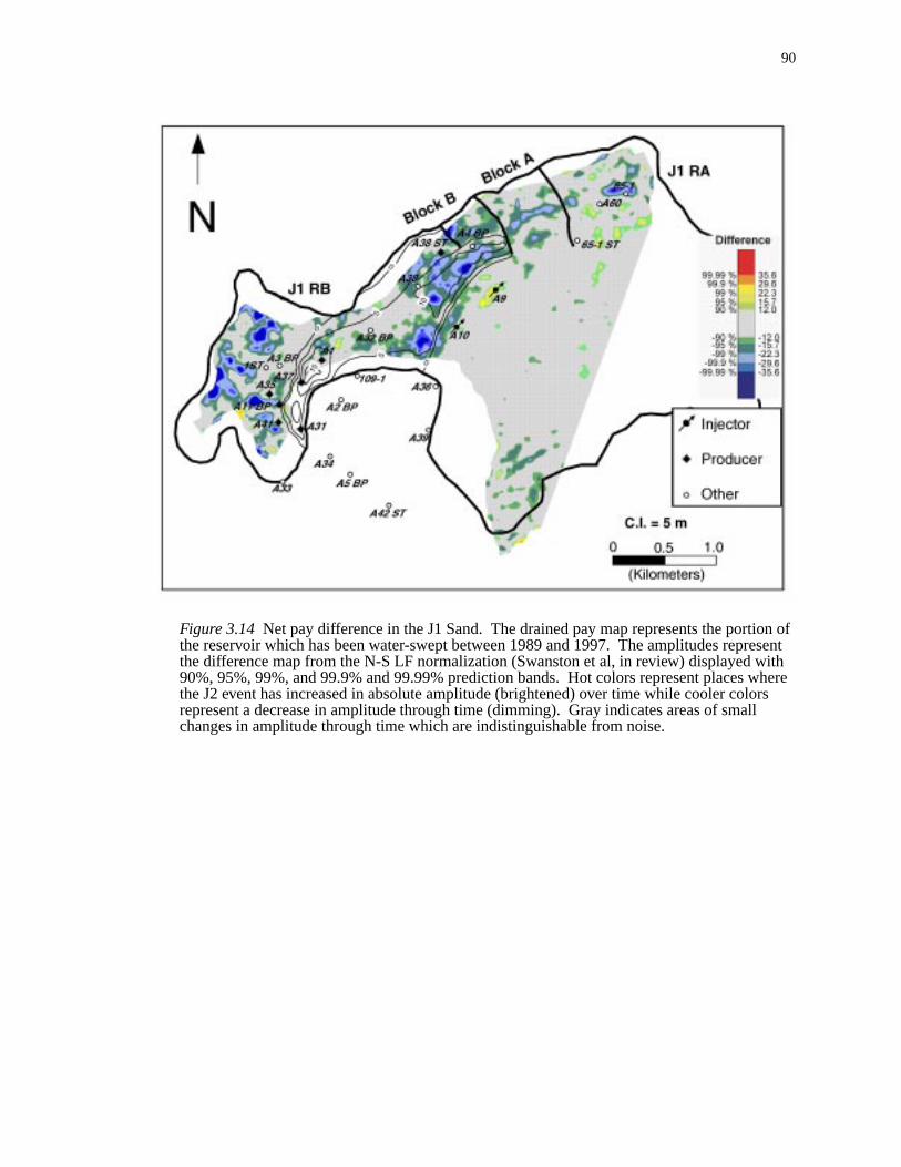
90

ion ofesentith

wherers

ll

Figure 3.14 Net pay difference in the J1 Sand. The drained pay map represents the portthe reservoir which has been water-swept between 1989 and 1997. The amplitudes reprthe difference map from the N-S LF normalization (Swanston et al, in review) displayed w90%, 95%, 99%, and 99.9% and 99.99% prediction bands. Hot colors represent places the J2 event has increased in absolute amplitude (brightened) over time while cooler colorepresent a decrease in amplitude through time (dimming). Gray indicates areas of smachanges in amplitude through time which are indistinguishable from noise.

91

ve

the

ble

il-

997

om

in

ser-

-ft of

an

istory

mes

calculated by subtracting the total amount of oil remaining in the reservoirs both abo

and below the 1997 OWC from the initial 1989 volumes.

We compared the volume of drained oil we calculated using our drainage model to

measured cumulative production from the J1 and J2 RB reservoirs through 1997 (Ta

3.1). Actual cumulative production of oil from both reservoirs totalled 68.8 MMstb (m

lions of stock tank barrels). Cumulative production of oil at reservoir conditions by 1

was 98.8 MMrb. Our drainage model predicts that 90 MMrb of oil were extracted fr

both reservoirs. The drainage model predicts the actual amount of oil produced with

8%. The recovery factor (RF) is a ratio of the drained oil volume to the volume of re

voir rock which has been water-swept in terms of stb/ac-ft (stock tank barrels per ac

reservoir). For the J1 and J2 RB, this number is equal to 1058 stb/ac-ft.

The drainage model which predicts actual produced volumes within 8% assumes

Sor of 0.25. There is some uncertainty regarding the exact values for Sor, although our

assumption of 0.25 agrees with core data. Best (2002) produced the most accurate h

match for the J1 and J2 simulation when he used an Sor of 0.25 in all flow units besides

Unit 4 (Figures 2.23 and 2.24). Best (2002) used an Sor of 0.11 in Unit 4. We used the

drainage analysis presented in Table 2.1 to determine an average Sor for the J1 and J2 RB

reservoirs which would result in a perfect match between our predicted drained volu

and observed produced oil volumes. An Sor of 0.20 is needed to exactly match the pro-

duced volumes to the observed produced volumes.

92

of

ted

ll

rvoir

ation

e gas

on is

cous-

per-

ered.

ease

tic

al.,

rent

the

e to

puts

ids,

ct the

re.

Gassmann Model

Saturation and pressure changes have a significant effect on acoustic velocity

unconsolidated reservoir sands (Domenico, 1977; Landro, 2001). In an undersatura

reservoir, an increase in Sw and decrease in So due to water sweep will increase the overa

acoustic velocity (Gregory, 1976). In the case where an initially undersaturated rese

drops below the bubble-point, gas saturation will increase. An increase in gas satur

will dramatically decrease the velocity because of the presence highly compressibl

in the pore space (Domenico, 1977; Whitman and Towle, 1992). Even when saturati

held constant, changes in the elastic properties of the saturating fluid also affect the a

tic velocity of a rock (Jones et al., 1988; Clark, 1992; Alberty, 1996). The elastic pro

ties of the rock frame also change when the effective stress state of the reservoir is alt

Rock property changes include porosity reduction and frame stiffening due to a decr

in reservoir pressure and increase in vertical effective stress (Landro, 2001). Acous

velocity will increase as the rock frame is stiffened and porosity is reduced (Wyllie et

1956; Christensen and Wang, 1985; Zhang and Bentley, 2000).

Gassmann fluid substitution modeling uses the elastic moduli of the dry rock to

describe the overall changes in acoustic velocity when that rock is saturated with diffe

fluids (Gassmann, 1951; Domenico, 1977; Mavko et al., 1995; Alberty, 1996). We use

Gassmann Equations to model changes in the acoustic properties of the J Sands du

production-related changes in reservoir pressure, effective stress, and saturation. In

into the Gassmann Equations include porosity and the moduli of the solid grains, flu

and dry rock. When those parameters are known, the Gassmann Equation will predi

bulk p-wave modulus of the saturated rock for any changes in saturation and pressu

93

ulk

mod-

e

Acoustic P-wave (Vp) velocity is then calculated from the bulk P-wave modulus and b

density of the saturated rock.

Gassmann (1951) formulated a relation between a saturated rock’s bulk p-wave

ulus (M) and its corresponding dry frame (Kdry), grain (Ko), and pore fluid (Kfl) moduli,

. (3.2)

The constant S depends on the dry rock Poisson’s ratio (ν),

. (3.3)

The modulus of the composite fluid mixture (Kfl) is determined using the Reuss average

(Dvorkin et al., 1999) of each fluid’s modulus (oil, gas, and water):

. (3.4)

Acoustic p-wave velocity (Vp) is related to the bulk p-wave modulus (M) solved in th

Gassmann Equation (Equation 3.2) and the bulk density (ρb):

. (3.5)

M SKdry

1Kdry

Ko-----------–

2

φK fl-------- 1 φ–( )

Ko----------------

Kdry

Ko2

-----------–+

-------------------------------------------------+=

S3 1 υ–( )

1 υ+( )--------------------=

1K fl--------

Sw

Kw-------

So

Koil---------

Sg

Kg------+ +=

VpMρb-----=

94

con-

d-

.2.

us

rela-

e rock

e the

es

e last

e

(1952)

count

ump-

ugh-

000).

a one-

For application of Equations 3.2 through 3.5, we need to know the basic elastic

stants of the rock and fluids. Ko is the modulus for pure quartz (38000 MPa). Fluid mo

uli for oil (Koil), gas (Kg), and water (Kw) were computed from known correlations

(Batzle and Wang, 1992). The dry rock poisson ratio (ν) is unknown and we assume a

value based on previous studies. Kdry is also unknown, but can be calculated when the

bulk density and Vp of a rock has been measured using Equation 3.5 with Equation 3

There are several assumptions when applying the Gassmann Equations to poro

rocks. The pores of the rock all must be interconnected and its fluid must not move

tive to the frame during the onset of an acoustic wave (Gassmann, 1951). Second, th

must be under undrained conditions, where pore fluids are not allowed to enter or leav

system. Third, the shear modulus (µ) is independent of fluid saturation and only chang

as a function of porosity and effective stress (Gassmann, 1951; Berryman, 1999). Th

assumption is that the pore fluid does not cause chemical changes in the rock’s fram

(Gassmann, 1952; Wang, 2000).

Frequency is also an issue when applying the Gassmann equations. Gassmann

derived his equations assuming zero-frequency (infinite wavelength) and does not ac

for dispersion. High porosity and permeability sands have been shown to fit the ass

tions of the Gassmann Equations because the fluids equilibrate and allow for flow thro

out the pore space during the onset of a compressional wave (Blangy, 1992; Wang, 2

For example, Blangy (1992) compared ultrasonic laboratory measurements of Vp in

unconsolidated sands with Gassmann predictions and showed that there is close to

to-one correlation.

95

a).

i/ft in

rved

ess is

her.

.

g of

pene-

ses

sim-

ver-

e

74)

80;

s in

s of

Porosity, Effective Stress, and Vp Observations

Porosity in the Bullwinkle J Sands is proportional to effective stress (Figure 3.15

Effective stress was calculated assuming a constant hydrostatic gradient of 0.465 ps

the water leg and a constant overpressure of 20.1 Mpa. Flemings et al. (2001) obse

higher porosities in the J3 sand at the top of structure where the vertical effective str

low and lower porosities at the base of the sand where vertical effective stress is hig

The dashed line in Figure 3.15a is the compaction trend observed by Flemings et al

(2001) for the J3 sand. The two wells with porosity logs that penetrated the water le

the J2 demonstrate that porosity in the J2 may also be stress-controlled. One well

trated the water leg of the J1 in the 65-1 (Figure 2.2)

Acoustic velocity (Vp) in the water leg of the J Sands increases as porosity decrea

(Figure 3.15b). A linear regression between porosity and Vp for all the data points shows

that Vp tends to be higher for sands with lower porosities. Blangy (1992) observed a

ilar trend in the Troll sands (dashed line in Figure 3.15b). The Troll sands are not o

pressured, but are at approximately the same effective stress state (~15 MPa) as th

Bullwinkle J Sands (Blangy, 1992). A universal trend observed by Gardner et al. (19

overpredicts porosity for the J Sands based on Vp. The Vp scale in Figure 3.15b is

expanded in Figure 3.15d to show how the Bullwinkle Vp/porosity relationship compares

with some other well known porosity transforms (Wyllie et al., 1956; Raymer et al., 19

Han et al., 1986). The Wyllie et al., Raymer et al., and Han et al. porosity transform

Figure 3.15d are all empirical and were derived in cemented and consolidated sand

various porosities. They all grossly underpredict the porosity/Vp behavior exhibited at

Bullwinkle because they were not meant to be applied to unconsolidated sands.

96

nity waswell

ments

Figure 3.15 Effective stress, porosity, and Vp observations from the Bullwinkle J Sands. Opecircles represent J3, black circles represent J2, and gray circle represents the J1. Poroscalculated from the RHOB log and an average value for DPHI and DT were taken in eachwhich penetrated each sand below the OWC. Effective stress for the J3 was taken fromFlemings et al., 2001. Effective stress in the J1 and J2 were inferred from RFT measurein the 109-1 J2 sands.

14 15 16 170.28

0.29

0.3

0.31

0.32

0.33

0.34

Vertical Effective Stress (Mpa)

Por

osity

A5 BP

A4 BP

65-1 ST

A36

A36

109-1 A2 BP

A32 BP

65-1 ST

0.30 0.32 0.342500

2550

2600

2650

2700

2750

Vp (

m/s

)Porosity

14 15 16 172500

2550

2600

2650

2700

2750

Vertical Effective Stress (Mpa)0.28 0.30 0.32 0.34

2200

2400

2600

2800

3000

3200

3400

3600

3800

65-1 ST

Blangy, 1992

Vp = 3384 - 2415φ R = 0.40

Wyllie et al. (1956)Raymer et al. (1980)Han et al. (1986)

Blangy (1992)

Gardner et al. (1974)

Gardner et al. (1974)

Porosity

Vp (

m/s

)

Vp (

m/s

)Flemings et al. (2001)

0.28

0.322

0.310

0.336

0.301

0.310

0.290

0.319

0.324

0.316

0.290

a) b)

c) d)

Vp = 63

σ + 16

70 R

= 0.

75

v

2

97

ss

and

nd

ction,

the

ress

y,

ant

-

tions

9).

a. A

Velocity in the water-saturated J Sands is strongly controlled by the effective stre

state (Figure 3.15c). Rocks at a lower effective stress overall have a higher porosity

lower Vp (Figure 3.15c) while rocks with higher effective stress have a lower porosity a

higher Vp. This behavior is important because it suggests that Vp will increase in the res-

ervoir as the pore pressure is reduced and effective stress is increased due to produ

even while saturations remain constant.

Porosity, Effective Stress and Kdry Observations

The key to understanding the behavior seen in Figure 3.15c is to recognize that

overall modulus (incompressibility) of a rock increases with an increase in effective st

(Gregory, 1976; Eberhart-Phillips et al., 1989). The incompressibility of the dry rock

devoid of fluids is termed Kdry and can be calculated from sonic log data when porosit

Ko, Kfl, andν are known from Equation 3.2. For the water leg data, we assumed that Ko =

38000 MPa (quartz), Kfl = 3800 MPa (brine with salinity of 220 kppm), andν = 0.18. Vp

, φ, andρb were taken from well log measurements (Table 3.3) We assumed a const

value for the dry rock poisson’s ratio (ν) of 0.18 because it is a typical value for uncon

solidated Gulf of Mexico reservoir sands (Spencer et al., 1994). Under these assump

Equation 3.2 is solved for Kdry in Table 3.3 using a method first developed by Gregory

(1977) and put to use in similar studies by Burkhart (1997) and Benson and Wu (199

The J Sand water-leg data show that Kdry increases at higher effective stress. Kdry in

Figure 3.16a ranges from 2.98 to 3.3 GPa over an effective stress interval of 2.2 MP

first order fit to the data in Figure 3.16a reveals a linear relationship between Kdry andσv

98

rclesin

ion.

Figure 3.16 Relationships between Kdry, effective stress and porosity for the Bullwinkle JSands. Open circles represent J3 sand, black circles represent J2 sand, and the gray cirepresents J1 sand well penetrations. a) Kdry as a function of effective stress using the data

Table 3.3. DPHI is labeled for each well penetration. A first order fit to all data give an R2 of0.61. b) Kdry as a function of porosity. The effective stress is labeled for each well penetrat

A first order fit to the data give an R2 of 0.21.

13 14 15 16 17

2.6

2.8

3.0

3.2

3.4

3.6

0.319

0.336

0.310

0.301

0.290

0.322

0.324

0.316

0.310

0.290

Vertical Effective Stress (MPa)

Kdr

y (G

Pa)

0.30 0.32 0.34

2.6

2.8

3.0

3.2

3.4

3.6

15

15.6

16

16.6

15.6

14.7

14.4

14.7

15.1

15

Porosity0.28

Kdr

y =

0.39

74*σ

- 2.

9284

R =

0.6

1

v

Kdry = -10.49φ + 6.4107 R = 0.21

a) b)

J1J2J3

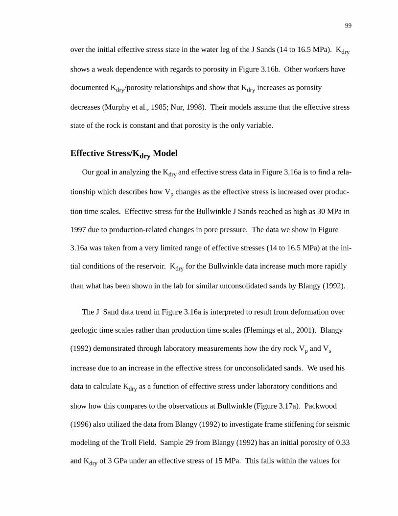
99

K

have

stress

la-

uc-

Pa in

ure

e ini-

92).

ver

ngy

ed his

d

mic

33

r

over the initial effective stress state in the water leg of the J Sands (14 to 16.5 MPa).dry

shows a weak dependence with regards to porosity in Figure 3.16b. Other workers

documented Kdry/porosity relationships and show that Kdry increases as porosity

decreases (Murphy et al., 1985; Nur, 1998). Their models assume that the effective

state of the rock is constant and that porosity is the only variable.

Effective Stress/Kdry Model

Our goal in analyzing the Kdry and effective stress data in Figure 3.16a is to find a re

tionship which describes how Vp changes as the effective stress is increased over prod

tion time scales. Effective stress for the Bullwinkle J Sands reached as high as 30 M

1997 due to production-related changes in pore pressure. The data we show in Fig

3.16a was taken from a very limited range of effective stresses (14 to 16.5 MPa) at th

tial conditions of the reservoir. Kdry for the Bullwinkle data increase much more rapidly

than what has been shown in the lab for similar unconsolidated sands by Blangy (19

The J Sand data trend in Figure 3.16a is interpreted to result from deformation o

geologic time scales rather than production time scales (Flemings et al., 2001). Bla

(1992) demonstrated through laboratory measurements how the dry rock Vp and Vs

increase due to an increase in the effective stress for unconsolidated sands. We us

data to calculate Kdry as a function of effective stress under laboratory conditions and

show how this compares to the observations at Bullwinkle (Figure 3.17a). Packwoo

(1996) also utilized the data from Blangy (1992) to investigate frame stiffening for seis

modeling of the Troll Field. Sample 29 from Blangy (1992) has an initial porosity of 0.

and Kdry of 3 GPa under an effective stress of 15 MPa. This falls within the values fo

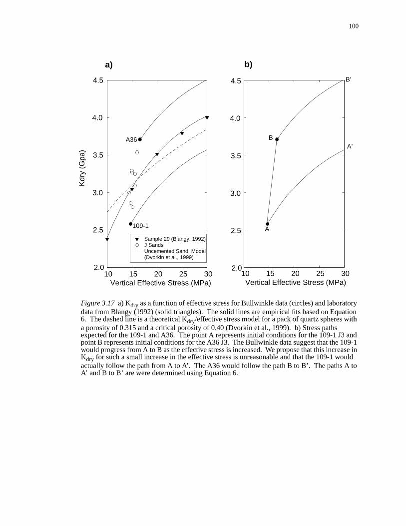
100

ryationth

and9-1

ase inould

o

Figure 3.17 a) Kdry as a function of effective stress for Bullwinkle data (circles) and laboratodata from Blangy (1992) (solid triangles). The solid lines are empirical fits based on Equ6. The dashed line is a theoretical Kdry/effective stress model for a pack of quartz spheres wia porosity of 0.315 and a critical porosity of 0.40 (Dvorkin et al., 1999). b) Stress pathsexpected for the 109-1 and A36. The point A represents initial conditions for the 109-1 J3point B represents initial conditions for the A36 J3. The Bullwinkle data suggest that the 10would progress from A to B as the effective stress is increased. We propose that this increKdry for such a small increase in the effective stress is unreasonable and that the 109-1 wactually follow the path from A to A’. The A36 would follow the path B to B’. The paths A tA’ and B to B’ are were determined using Equation 6.

10 15 20 25 302.0

2.5

3.0

3.5

4.0

4.5


Kdr

y (G

pa)

Sample 29 (Blangy, 1992)J SandsUncemented Sand Model (Dvorkin et al., 1999)

10 15 20 25 30Vertical Effective Stress (MPa)

A

A’B

B’

a) b)

2.0

2.5

3.0

3.5

4.0

4.5

109-1

A36

101

ffective

.17a

hang

rela-

the

sing

for

797,

edict

Kdry we calculated from the sonic log data for the J Sands at ~15 MPa. Kdry increased for

the sample as the effective stress increased and reached as high as 4 GPa under an e

stress of 30 MPa. The rate at which Kdry increased for Sample 29 was much less than

what is suggested by the Bullwinkle data (open circles). The solid lines in Figures 3

and 3.17b are empirical fits to the Blangy (1992) data using a method proposed by Z

and Bentley (2000).

Zhang and Bentley (2000) used the data of Han et al. (1985) to derive empirical

tions between Kdry and effective stress. They show that the change in Kdry as a function of

the effective stress could be approximated by

, (3.6)

where A and B are empirically derived constants, Kdry is in GPa andσv is in MPa. Inte-

gration of Equation 5 allows for Kdry to be solved for any effective stress,

, (3.7)

where C is a constant from the integration. Zhang and Bentley (2000) show that for

data of Han et al., 1985, A = 0.746 and B = -0.0773. They then tested Equation 3.7 u

the data of Gregory, 1977 and found that it predicted Kdry within 10 %.

We used the Blangy (1992) data in Figure 3.17a to derive the constants A and B

Equation 3.7. The constants A and B for the Blangy (1992) data are 0.362 and -0.0

respectively. The constant C for the Blangy (1992) data was calculated since Kdry is

known at 10 MPa. We then used our values for A and B along with Equation 6 to pr

Kdryd

σvd-------------- Ae

Bσv=

KdrydAB---e

Bσv C+=

102

ate C

arate

ur

.17b.

effec-

posed

ath of

er

how

to 30

ed

m-

al

the Kdry behavior of the 109-1 and A36, using the data in Table 3.3 to derive a separ

for each well. Solving for a separate value for C allows us to exactly match the Kdry at ini-

tial conditions for both the 109-1 and A36, and then model the rock’s stress path sep

from one another.

The stress path taken by the 109-1 and A36 data points will differ according to o

model (Figure 3.17b). For the 109-1 at initial conditions,σv = 14.7 MPa and Kdry = 2.5

GPa. The in-situ measurements of Kdry in the Bullwinkle J Sands as a function of effec-

tive stress would suggest that the 109-1 would take the stress path A to B on Figure 3

We propose that production related changes rock properties due to the increase in

tive stress take place over time scales much closer to laboratory measurements as op

to geologic time. Under production-induced changes in effective stress, the stress p

the 109-1 would be to follow A to A’ (Figure 3.17b). Rocks which are initially at a high

effective stress state (A36 in Figure 3.17a), will take the path B to B’. Both models s

an increase of Kdry between 1.5 and 2.0 GPa as the effective stress increases from 15

MPa.

Velocity Model for Water-Saturated Rocks Under Pressure

The Kdry relationship we found for the 109-1 and A36 wells in Figure 3.17a was us

to model how Vp increased in rocks 100% saturated with water as the effective stress

increased from 15 to 30 MPa. Vp was calculated using Equations 3.2 through 3.5 assu

ing Kfl = 3800 MPa and Ko = 38000 MPa. Kdry was calculated for each well, using the

paths A to A’ and B to B’ in Figure 3.17b for the 109-1 and A36, respectively. At initi

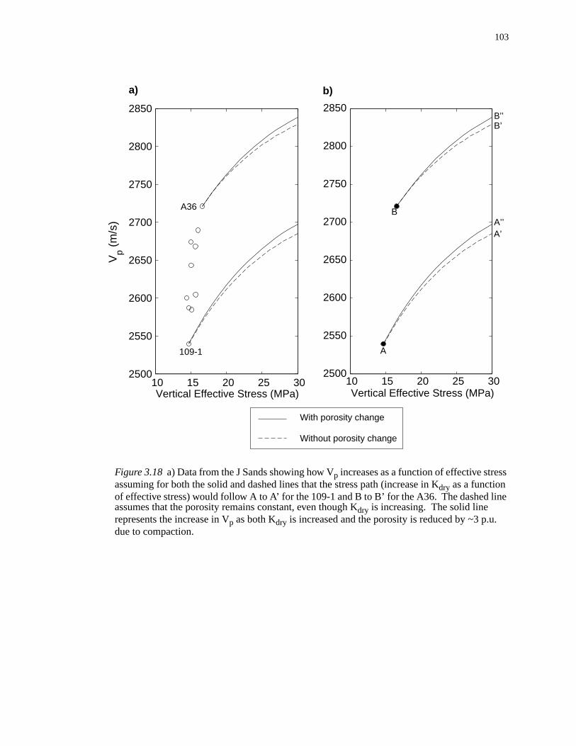
103

s

e

.

Figure 3.18a) Data from the J Sands showing how Vp increases as a function of effective stresassuming for both the solid and dashed lines that the stress path (increase in Kdry as a functionof effective stress) would follow A to A’ for the 109-1 and B to B’ for the A36. The dashed linassumes that the porosity remains constant, even though Kdry is increasing. The solid linerepresents the increase in Vp as both Kdry is increased and the porosity is reduced by ~3 p.udue to compaction.

10 15 20 25 302500

2550

2600

2650

2700

2750

2800

2850


Vp (

m/s

)

10 15 20 25 302500

2550

2600

2650

2700

2750

2800

2850


A

A’A’’

B

B’B’’

109-1

A36

a) b)

With porosity change

Without porosity change

104

ir-

d

ased

to

e

to

odu-

le

er

how

h a

f

conditions for both wells, Kdry is taken from Table 3.2, and corresponds to the black c

cles in Figure 3.18a.

We calculated Vp under two conditions (Figure 3.18a). For the first condition, we

model the change in Kdry as shown in Figure 3.17b, but keep porosity constant (dashe

lines in Figure 3.18a). For the second condition, we model the change in Kdry as shown in

Figure 3.17b, but also decrease the porosity by 3 p.u. as the effective stress is incre

from 15 to 30 MPa (solid lines in Figure 3.18). This porosity reduction corresponds

pore compressibility of 50x10-6 psi-1 . Vp in both the 109-1 and A36 increases as the

effective stress and Kdry increase. Overall, we observe about 200 m/s increase in Vp using

this model as each well travels from A to A’ and B to B’ in Figure 3.18b. If we assum

that porosity reduction is occurring in addition to frame stiffening, we show that Vp

increases by ~10 m/s more than it would if we kept porosity constant (A to A’’ and B

B’’ in Figure 3.18b).

Saturation Effects on Velocity and Seismic Amplitude

The saturated bulk modulus of unconsolidated sands is highly dependent on the m

lus of the saturating fluid (Gregory, 1976; Domenico, 1977; Alberty, 1997). Bullwink

oils have moduli which are ~1/3 that of brine. As a result, oil sands have a much low

value for Vp, impedance and higher absolute value for RFC than brine sands. We s

the effect of saturation on Vp, acoustic impedance, and RFC by considering a rock wit

Kdry of 2570 MPa and a porosity of 0.31 (Figure 3.19). Vp was calculated over a range o

water saturations using Equations 3.2 through 3.5. Porosity and Kdry were kept constant.

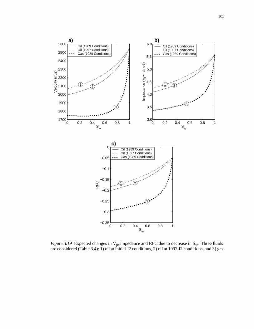
105

gas.
Figure 3.19 Expected changes in Vp, impedance and RFC due to decrease in Sw. Three fluidsare considered (Table 3.4): 1) oil at initial J2 conditions, 2) oil at 1997 J2 conditions, and 3)
0 0.2 0.4 0.6 0.8 11700

1800

1900

2000

2100

2200

2300

2400

2500

2600

Sw

Vel

ocity

(m

/s)

0 0.2 0.4 0.6 0.8 1−0.35

−0.3

−0.25

−0.2

−0.15

−0.1

−0.05

0

Sw

RF

C

0 0.2 0.4 0.6 0.8 13.0

3.5

4.0

4.5

5.0

5.5

6.0

Sw

Impe

danc

e (k

g−m

/s e

6)

a) b)

c)

12

3

1 2

3

1 2

3

Oil (1989 Conditions)Oil (1997 Conditions)Gas (1989 Conditions)



106

ure has

xpand,

ion

he

for a

d has

the

modu-

d rock

Case #1 represents the J2 in the 109-1 at initial conditions where Koil = 1300 MPa. Case

#2 represents that same sand, this time with a lighter oil (Koil = 1050 MPa). The lighter oil

in Case #2 has the same GOR as the oil in Case #1, except that the reservoir press

been decreased by 15 MPa. This decrease in reservoir pressure causes the oil to e

which in turn causes it to have a lower density and Koil (Batzle and Wang, 1992). Case #3

is a gas sand with no oil present.

Gassmann fluid substitution in Figure 3.19 shows that both fluid type and saturat

have a significant effect on the acoustic signature of the reservoir. At an Sw = 1, all three

cases show the same values because the rock is 100% saturated with water. As Sw

decreases and the hydrocarbon saturation increases, Vp and impedance decrease and the

magnitude of the RFC increases for all 3 cases.

The degree to which the acoustic properties of the rock change is controlled by t

fluid type (Figure 3.19). For Case #1, velocity decreased from 2550 m/s to 2080 m/s

saturation change from 1 to 0. Impedance decreased from 5.50 to 4.25 kg/m2s x 106. The

RFC changed from -0.05 to -0.18 as the oil saturation increased (Sw decreased). For Case

#2, Vp at 100% oil saturation was 80 m/s less than it was for Case #1. The lower Vp at

100% oil saturation occurs because the hydrocarbon saturating the pores is lighter an

a lower modulus. The lower Vp for Case #2 decreased the impedance by 2 kg/m2s x 106

and increased the magnitude of the RFC by 0.02. The gas sand in Case #3 showed

greatest impact on the acoustic properties because gas has much lower density and

lus than oil. For Case #3, as the gas saturation increased from a 100% brine saturate

107

is

5.

hit-

idly

e and

was

ce

by as

rby

9-1

tion

ining

to 20% gas saturation (0.80 Sw), Vp decreased from 2550 m/s to 1850 m/s. Impedance

also drastically dropped from 5.5 to 3.4 kg/m2s x 106 as the gas saturation increased. Th

large difference in the impedance then increased the magnitude of the RFC to -0.29

Changes in Vp for Case #3 shows at first some non-intuitive behavior at lower Sw. Vp

actually starts to increase slightly as Sw is reduced from 0.30 to 0 (Figure 3.19a). This

behavior has been documented by Domenico (1977) in the lab and is explained by W

man and Towle (1992) in terms of Equation 3.5. At higher Sw, as the gas saturation

increases (Sw decreases), the p-wave modulus (M) of the rock decreases more rap

than the bulk density. The slight increase in Vp from Sw = 0.3 to Sw = 0 occurs because

the bulk density now is decreasing faster than the p-wave modulus. Both impedanc

RFC still show a decrease as Sw decreases (Figure 3.19b,c)

Coupled Pressure and Saturation Effects on the Acoustic Properties

Model of Acoustic Response due to Water Sweep and Changes in Effective Stress

We consider first the acoustic property changes in the 109-1 J2, where the sand

initially oil-saturated in 1989 and then water swept by 1997. The time-lapse differen

amplitude map in Figure 3.13 shows that the 109-1 area had decreased in amplitude

much as 70% between 1989 and 1997. Production and PNC log data from the nea

A32 BP well (Figures 3.3, 3.5, 3.6, and 3.7) show that the OWC had reached the 10

level by 1994. Initial porosity in the 109-1 J2 has an average value of 0.31. Compac

due to an increase in effective stress reduced the porosity to 0.28 by 1997. The rema

rock and fluid properties are summarized in Table 3.5.

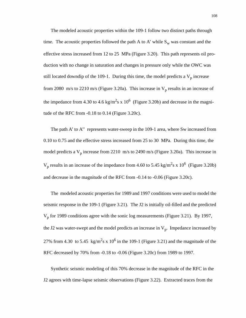
108

h

il pro-

as

-

from

, the

e in

el the

ted

97,

e

the

the

The modeled acoustic properties within the 109-1 follow two distinct paths throug

time. The acoustic properties followed the path A to A’ while Sw was constant and the

effective stress increased from 12 to 25 MPa (Figure 3.20). This path represents o

duction with no change in saturation and changes in pressure only while the OWC w

still located downdip of the 109-1. During this time, the model predicts a Vp increase

from 2080 m/s to 2210 m/s (Figure 3.20a). This increase in Vp results in an increase of

the impedance from 4.30 to 4.6 kg/m2s x 106 (Figure 3.20b) and decrease in the magni

tude of the RFC from -0.18 to 0.14 (Figure 3.20c).

The path A’ to A’’ represents water-sweep in the 109-1 area, where Sw increased

0.10 to 0.75 and the effective stress increased from 25 to 30 MPa. During this time

model predicts a Vp increase from 2210 m/s to 2490 m/s (Figure 3.20a). This increas

Vp results in an increase of the impedance from 4.60 to 5.45 kg/m2s x 106 (Figure 3.20b)

and decrease in the magnitude of the RFC from -0.14 to -0.06 (Figure 3.20c).

The modeled acoustic properties for 1989 and 1997 conditions were used to mod

seismic response in the 109-1 (Figure 3.21). The J2 is initially oil-filled and the predic

Vp for 1989 conditions agree with the sonic log measurements (Figure 3.21). By 19

the J2 was water-swept and the model predicts an increase in Vp. Impedance increased by

27% from 4.30 to 5.45 kg/m2s x 106 in the 109-1 (Figure 3.21) and the magnitude of th

RFC decreased by 70% from -0.18 to -0.06 (Figure 3.20c) from 1989 to 1997.

Synthetic seismic modeling of this 70% decrease in the magnitude of the RFC in

J2 agrees with time-lapse seismic observations (Figure 3.22). Extracted traces from

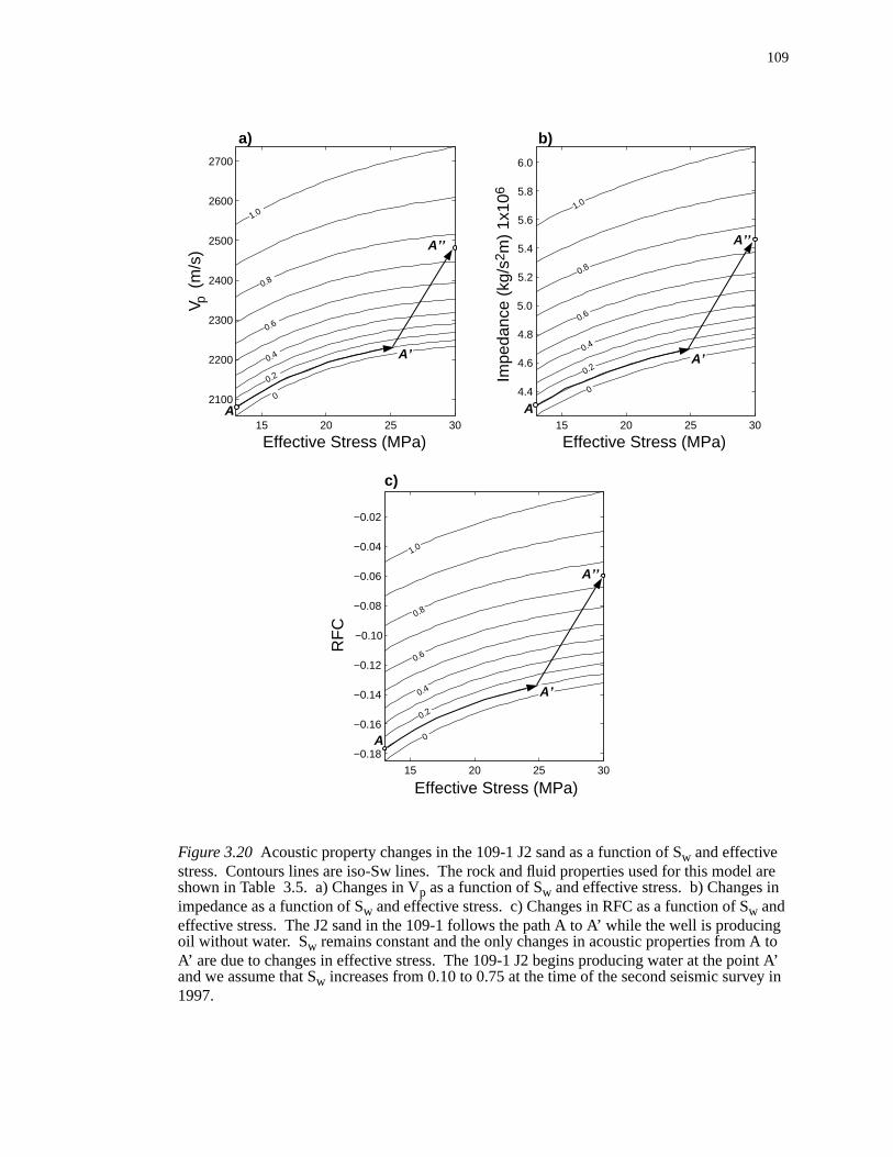
109

l are

cing toint A’y in

Figure 3.20 Acoustic property changes in the 109-1 J2 sand as a function of Sw and effectivestress. Contours lines are iso-Sw lines. The rock and fluid properties used for this modeshown in Table 3.5. a) Changes in Vp as a function of Sw and effective stress. b) Changes inimpedance as a function of Sw and effective stress. c) Changes in RFC as a function of Sw andeffective stress. The J2 sand in the 109-1 follows the path A to A’ while the well is produoil without water. Sw remains constant and the only changes in acoustic properties from AA’ are due to changes in effective stress. The 109-1 J2 begins producing water at the poand we assume that Sw increases from 0.10 to 0.75 at the time of the second seismic surve1997.

15 20 25 30

2100

2200

2300

2400

2500

2600

2700

15 20 25 30

−0.18

−0.16

−0.14

−0.12

−0.10

−0.08

−0.06

−0.04

−0.02

15 20 25 30

4.4

4.6

4.8

5.0

5.2

5.4

5.6

5.8

6.0

0

0.2

0.4

0.6

0.8

1.0

0

0.2

0.4

0.6

0.8

1.0

0

0.2

0.4

0.6

0.8

1.0

a) b)

c)

A

A’’

A

A’’

A

A’’

A’

A’ A’

Effective Stress (MPa) Effective Stress (MPa)

Impe

danc

e (k

g/s2

m)

1x10

6

Effective Stress (MPa)

RF

C

V (

m/s

)p

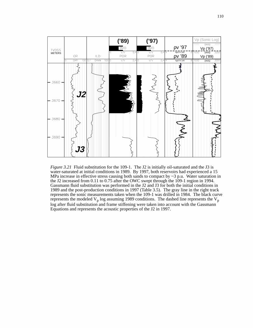
110

15tion in4. inckcurve

Vn

Figure 3.21 Fluid substitution for the 109-1. The J2 is initially oil-saturated and the J3 iswater-saturated at initial conditions in 1989. By 1997, both reservoirs had experienced aMPa increase in effective stress causing both sands to compact by ~3 p.u. Water saturathe J2 increased from 0.11 to 0.75 after the OWC swept through the 109-1 region in 199Gassmann fluid substitution was performed in the J2 and J3 for both the initial conditions1989 and the post-production conditions in 1997 (Table 3.5). The gray line in the right trarepresents the sonic measurements taken when the 109-1 was drilled in 1984. The blackrepresents the modeled Vp log assuming 1989 conditions. The dashed line represents the plog after fluid substitution and frame stiffening were taken into account with the GassmanEquations and represents the acoustic properties of the J2 in 1997.

Vp (Sonic Log)(m/s)

Vp (’89)

Vp (’97)

(’89) (’97)

J2

J3

(m/s)

(m/s)

ρv ’97

ρv ’89METERS

kg/s m 1e62

kg/s m 1e62

111

the

aree wasre

ch lies and

Figure 3.22 Seismic model for water-sweep in the 109-1 J2 sand. a) Extracted traces fromNS LF normalization (Swanston et al, in review) and synthetic traces obtained from fluidsubstitution modeling. b) Observed seismic difference from the N-S LF normalizationcompared with the modeled synthetic difference. RFC calculated under 1989 conditionsshown as the gray bars while RFC under 1997 conditions are solid black bars. Impedanccalculated from the modeled Vp and RHOB logs. The gray boxes which overlie the traces athe prediction bands as calculated by Swanston et al. (in review). Seismic differences whioutside the box are statistically shown to be caused by changes in rock and fluid propertienot noise (Burkhart et al., 1999; Swanston et al., in review).

NSLF ’89 Synth ’89 NSLF ’97 Synth ’97METERS

J2

J3

NSLF Diff.

Synth Diff.

METERS

J2

J3

a)

b)

Imped. (’97)

Imped. (’88) RFC (’88)

RFC (’97)kg-m/s 1e6

kg-m/s 1e6

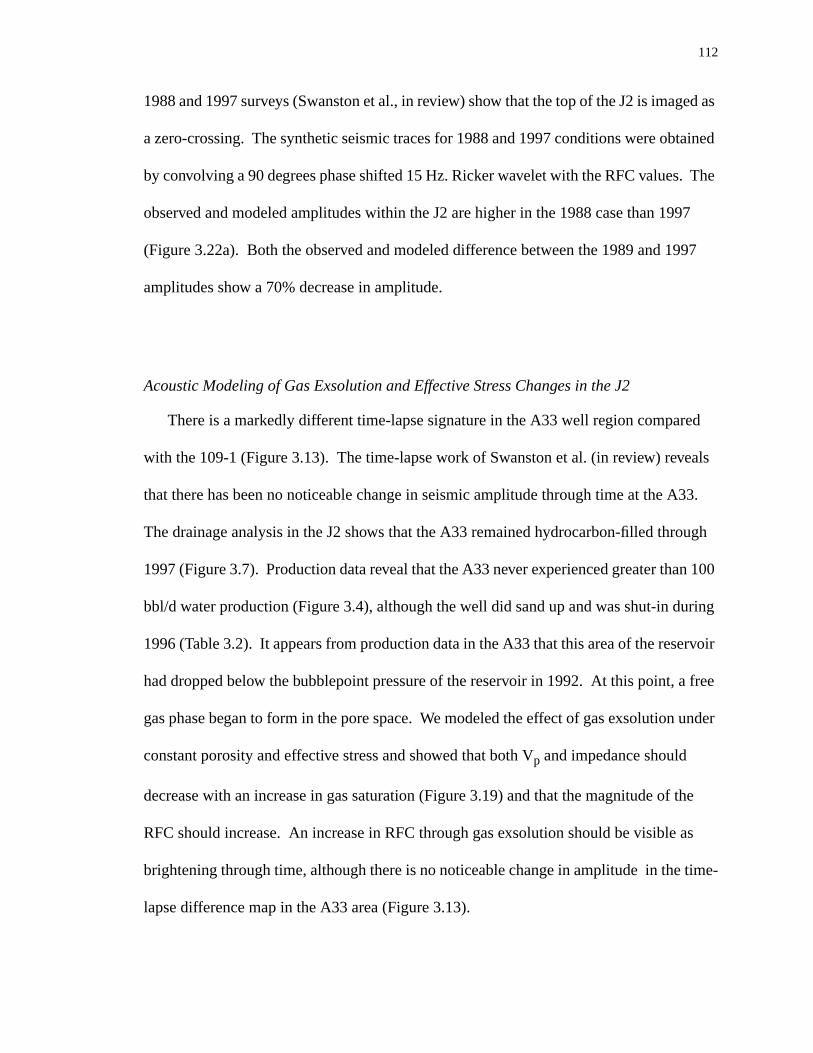
112

ed as

ained

The

97

997

ed

eals

33.

ugh

n 100

ring

rvoir

free

under

the

as

time-

1988 and 1997 surveys (Swanston et al., in review) show that the top of the J2 is imag

a zero-crossing. The synthetic seismic traces for 1988 and 1997 conditions were obt

by convolving a 90 degrees phase shifted 15 Hz. Ricker wavelet with the RFC values.

observed and modeled amplitudes within the J2 are higher in the 1988 case than 19

(Figure 3.22a). Both the observed and modeled difference between the 1989 and 1

amplitudes show a 70% decrease in amplitude.

Acoustic Modeling of Gas Exsolution and Effective Stress Changes in the J2

There is a markedly different time-lapse signature in the A33 well region compar

with the 109-1 (Figure 3.13). The time-lapse work of Swanston et al. (in review) rev

that there has been no noticeable change in seismic amplitude through time at the A

The drainage analysis in the J2 shows that the A33 remained hydrocarbon-filled thro

1997 (Figure 3.7). Production data reveal that the A33 never experienced greater tha

bbl/d water production (Figure 3.4), although the well did sand up and was shut-in du

1996 (Table 3.2). It appears from production data in the A33 that this area of the rese

had dropped below the bubblepoint pressure of the reservoir in 1992. At this point, a

gas phase began to form in the pore space. We modeled the effect of gas exsolution

constant porosity and effective stress and showed that both Vp and impedance should

decrease with an increase in gas saturation (Figure 3.19) and that the magnitude of

RFC should increase. An increase in RFC through gas exsolution should be visible

brightening through time, although there is no noticeable change in amplitude in the

lapse difference map in the A33 area (Figure 3.13).

113

ction

ges in

lution

n stiff-

. We

ove

the

.7)

gan to

point

corre-

tant,

gas

n the

We propose for the A33 that the competing effects of gas exsolution and compa

cause no detectable changes in the acoustic impedance and RFC. These two chan

rock and fluid properties have opposite effects on the acoustic properties. Gas exso

decreases the impedance and increases the magnitude of the RFC while compactio

ens the rock and increases the impedance while reducing the magnitude of the RFC

use the Gassmann Equations coupled with the Kdry model in Figure 3.17 to show that it is

possible to explain the time lapse signature in Figure 3.13.

The Gassmann model for the A33 predicts an increase in Vp and impedance while the

reservoir remains undersaturated (Figure 3.23). Initially, the reservoir pressure is ab

the bubblepoint (Table 3.6). From 1989 to 1992, the acoustic properties follow along

path A to A’ in Figure 3.23. Along A to A’, there are no changes in saturation (Table 3

and the effective stress increases from 10 to 20 MPa. The modeled Vp increases from

2030 m/s to 2210 m/s due to changes in the effective stress only. This increase in Vp

results in an increase of the impedance from 4.31 to 4.75 kg/s2m x 106 (Figure 3.23b) and

decrease in the magnitude of the RFC from -0.19 to -0.145 (Figure 3.23c).

The acoustic properties changed drastically in the A33 once a free gas phase be

form. Gas exsolution began when the reservoir pressure dropped below the bubble

pressure in 1992 and the reservoir entered the saturated region of Figure 3.23. This

sponds to an effective stress of 20 MPa (Figure 3.23). At this point, Sw remains cons

but the gas saturation (Sg) increases. For any given effective stress, Vp and impedance

decrease as Sg increases. Vp and impedance decrease because the presence of a free

phase reduces the bulk modulus of the rock. There is uncertainty in Sg in 1997 whe

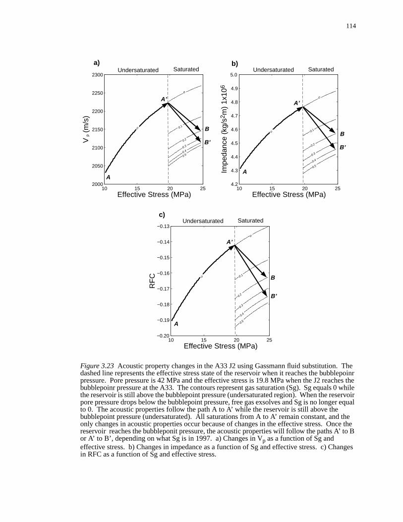
114

Thelepoinrhes thewhile

ervoirr equal

thece the

’ to B

hanges

Figure 3.23 Acoustic property changes in the A33 J2 using Gassmann fluid substitution. dashed line represents the effective stress state of the reservoir when it reaches the bubbpressure. Pore pressure is 42 MPa and the effective stress is 19.8 MPa when the J2 reacbubblepoinr pressure at the A33. The contours represent gas saturation (Sg). Sg equals 0the reservoir is still above the bubblepoint pressure (undersaturated region). When the respore pressure drops below the bubblepoint pressure, free gas exsolves and Sg is no longeto 0. The acoustic properties follow the path A to A’ while the reservoir is still above thebubblepoint pressure (undersaturated). All saturations from A to A’ remain constant, andonly changes in acoustic properties occur because of changes in the effective stress. Onreservoir reaches the bubbleponit pressure, the acoustic properties will follow the paths Aor A’ to B’, depending on what Sg is in 1997. a) Changes in Vp as a function of Sg andeffective stress. b) Changes in impedance as a function of Sg and effective stress. c) Cin RFC as a function of Sg and effective stress.

B

B’

a) b)

A’

10 15 20 252000

2050

2100

2150

2200

2250

2300


pV

(m

/s)

10 15 20 254.2

4.3

4.4

4.5

4.6

4.7

4.8

4.9

5.0


Impe

danc

e (k

g/s2

m)

1x10

6

0

0

0.2

0.3

0.4

0.5

A

B0.1

B’

c)

0

0.2

0.3

0.4

0.5

0.1

A’

A

0

Undersaturated Saturated Undersaturated Saturated

10 15 20 25−0.20

−0.19

−0.18

−0.17

−0.16

−0.15

−0.14

−0.13


RF

C

0

0.2

0.3

0.4

0.5

0.1

A’

B

B’

A

0

Undersaturated Saturated

115

nd Sg

.20

oth

.24b).

atch

been

ismic

both

erty

pres-

e 15

ective

tant

s at

he

el

A33 has reached an effective stress of 25 MPa, so we consider two cases: Sg = 0.20 a

= 0.40. The acoustic properties of the reservoir will follow the path A’ to B for Sg = 0

or A to B’’ for Sg = 0.40 when an effective stress of 25 MPa is reached in 1997.

The seismic modeling for the A33 includes the two cases shown in Figure 3.23. B

cases predict very little change in the impedance between 1989 and 1997 (Figure 3

Synthetic seismograms computed from the model for the 1989 and 1997 conditions m

actual seismic traces (Figure 3.24a). It is apparent from Figure 3.24a that there has

very little change in the seismic amplitude between 1989 and 1997. The modeled se

responses for both cases agree with the observed difference (Figure 3.24b).

Summary of Gassmann Model

The acoustic properties of the J2 sand were calculated as a function of depth at

initial (1989) and post-production (1997) conditions (Figure 3.25). The acoustic prop

profiles in Figure 3.24 were constructed using Equations 3.2 through 3.5. Reservoir

sure decreased by 15 MPa due to production of fluids between 1989 and 1997. Th

MPa decrease in reservoir pressure resulted in a 15 MPa increase in the vertical eff

stress. Initial porosity in 1989 is held constant as a function of depth at 0.32 and

decreased to 0.28 by 1997 as a result of compaction. Water saturation is held cons

above the OOWC in 1989 at 0.15. Water saturation above the OWC in 1997 remain

0.15 while Sw in the water-swept zone changes from 0.15 in 1989 to 0.75 in 1997. T

dry rock modulus (Kdry) was calculated as a function of effective stress using the mod

presented in Figure 3.17.

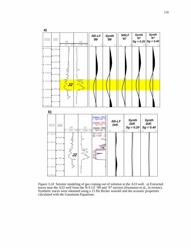
116

).
Figure 3.24 Seismic modeling of gas coming out of solution in the A33 well. a) Extractedtraces near the A33 well from the N-S LF ‘89 and ‘97 surveys (Swanston et al., in reviewSynthetic traces were obtained using a 15 Hz Ricker wavelet and the acoustic propertiescalculated with the Gassmann Equations.
NS-LF ’89

Synth ’89

NSLF ’97

Synth ’97Sg = 0.20

J2

Synth ’97Sg = 0.40

a)

NS-LF Diff.

Synth Diff.Sg = 0.20

METERS

Imped. (’97)

Imped. (’97)

kg/s m 1e62

Imped. (’89)

kg/s m 1e62

kg/s m 1e62

Synth Diff.Sg = 0.40

Sg = 0.20Sg = 0.40

b)

J2

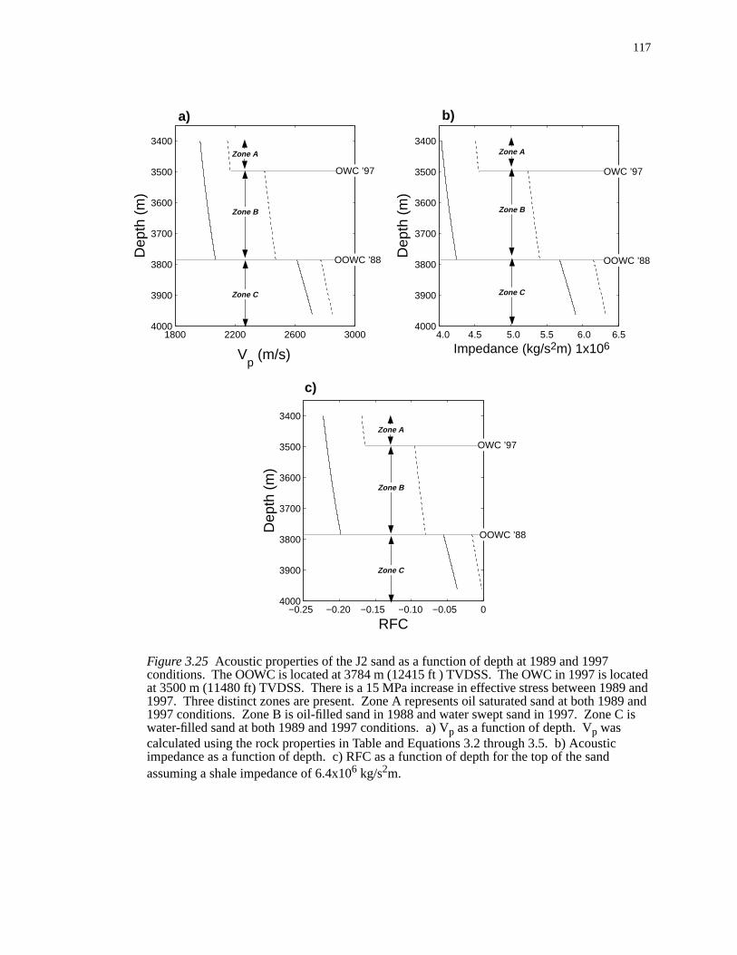
117

ted9 and89 and is

Figure 3.25 Acoustic properties of the J2 sand as a function of depth at 1989 and 1997conditions. The OOWC is located at 3784 m (12415 ft ) TVDSS. The OWC in 1997 is locaat 3500 m (11480 ft) TVDSS. There is a 15 MPa increase in effective stress between 1981997. Three distinct zones are present. Zone A represents oil saturated sand at both 191997 conditions. Zone B is oil-filled sand in 1988 and water swept sand in 1997. Zone Cwater-filled sand at both 1989 and 1997 conditions. a) Vp as a function of depth. Vp wascalculated using the rock properties in Table and Equations 3.2 through 3.5. b) Acousticimpedance as a function of depth. c) RFC as a function of depth for the top of the sandassuming a shale impedance of 6.4x106 kg/s2m.

−0.25 −0.20 −0.15 −0.10 −0.05 0

3400

3500

3600

3700

3800

3900

4000

Dep

th (

m)

RFC

OOWC ’88

OWC ’97

c)

4.0 4.5 5.0 5.5 6.0 6.5

3400

3500

3600

3700

3800

3900

4000

Dep

th (

m)

OOWC ’88

OWC ’97

Impedance (kg/s2m) 1x106

b)

Zone A

Zone B

Zone C

Zone A

Zone B

Zone C

1800 2200 2600 3000

3400

3500

3600

3700

3800

3900

4000

Dep

th (

m)

Vp (m/s)

OOWC ’88

OWC ’97

a)

Zone A

Zone B

Zone C

118

itial

gly.

. We

time,

and

ges

e pre-

neral

lysis

ly

ear the

fluid

sent in

s. Sat-

of

d in

effec-

. By

in V

Best (2002) demonstrated that oil composition varies as a function of depth at in

conditions for the J2 and we model the initial acoustic properties of the fluids accordin

Oil properties also change through time as a result of decreasing reservoir pressure

assume that the oil composition as a function of depth do not change as a function of

but vary properties as a function of reservoir pressure using the correlations of Batzle

Wang (1992).

The model we present in Figure 3.25 is a general summary of the acoustic chan

throughout the field and does not exactly reflect the detailed rock physics analysis w

sented for the 109-1 (Figure 3.20) and for the A33 (Figure 3.23). For example, the ge

model in Figure 3.25 does not take into account the formation of a gas cap like the ana

for the A33 in Figure 3.23. We assume for the general model that gas exsolution on

occured in localized areas, such as the A33, because of an increased pressure drop n

wellbore.

Acoustic properties in the J2 sand vary as a function of depth due to changes in

type, saturation, reservoir pressure, and effective stress. Three distinct zones are pre

Figure 3.25. Zone A represents oil-saturated sand at both 1989 and 1997 condition

uration remains constant in Zone A, although the oil properties do vary as a function

reservoir pressure (Batzle and Wang, 1992). Zone B represents initially oil-filled san

1989 and water-swept sand in 1997. Zone C represents the water leg.

Acoustic properties change in Zone A due to changes in reservoir pressure and

tive stress. In 1989, Vp ranges from 1970 to 1990 m/s (Figure 3.25a). Vp varies as a

function of depth in Zone A because oil density and GOR as also functions of depth

1997, Vp increased by 10% due to changes in reservoir pressure. The 10% increasep

119

ase in

erties

n

e

FC at

ming

effec-

d-

resulted in a 12% increase in the acoustic impedance (Figure 3.25b) and 25% decre

the RFC (Figure 3.25c).

Zone B is the water-swept zone and exhibits the greatest changes in acoustic prop

from 1989 to 1997 (Figure 3.25). In 1989, Zone B is initially oil-filled and Vp ranges from

1990 to 2070 m/s (Figure 3.25a). By 1997, Zone B experienced water-sweep and a

increase in effective stress. Vp increased by 20% in between 1989 and 1997 (Figure

3.25a). The 20% increase in Vp also increased the acoustic impedance by 28% (Figur

3.25b) and decreased the RFC by 60% (Figure 3.25c). The 60% decrease in the R

the top of the sand between 1989 and 1997 produced the wide areas of seismic dim

seen in Figure 3.13.

Zone C experiences no saturation or fluid property changes, although changes in

tive stress still effect the acoustic properties (Figure3.25). Vp ranges from 2613 and 2716

m/s in 1989. As the effective stress increases, Vp increases by 5% and the acoustic impe

ance increases by 8%.

120

as

duc-

n the

ntal

97.

and

e of

dicted

rame

ch as

d in a

iew).

1997

fluid

that

-lapse

sfully

Conclusions

We show that the OOWC in the J2 migrated upstructure from 3784 m to as high

3500 m TVDSS between 1989 and 1997. This movement of the OWC was due to pro

tion of oil from the J1 and J2 reservoirs and the encroachment of water from below i

aquifer. PNC log and production data also show that the OWC did not remain horizo

through 1997 and that small areas of undrained pay remained below the OWC in 19

The drainage model we formulate predicted that 90 MMrb were produced from the J1

J2 RB reservoir between 1989 and 1997. This value is within 8% of the actual volum

produced fluids (97.8 MMrb).

Gassmann fluid substitution of water sweep and gas exsolution successfully pre

the time-lapse changes observed by Swanston et al. (in review). We show that both f

stiffening, compaction, and water sweep increase the acoustic impedance by as mu

27% between 1989 and 1997. This 27% increase in the acoustic impedance resulte

70% decrease in the seismic amplitude which was observed by Swanston et al. (in rev

Production data suggested that free gas began exsolving in the area of the A33 before

and time-lapse data show no significant changes in amplitude. We used Gassmann

substitution to show that the frame stiffening effects cancelled out the gas effect and

between 1989 and 1997, the acoustic impedance only decreased slightly in the A33

region. The small changes in acoustic impedance resulted in a non-detectable time

signature, which was observed by Swanston et al. (in review) in the A33 and succes

modeled using the Gassmann Equations.

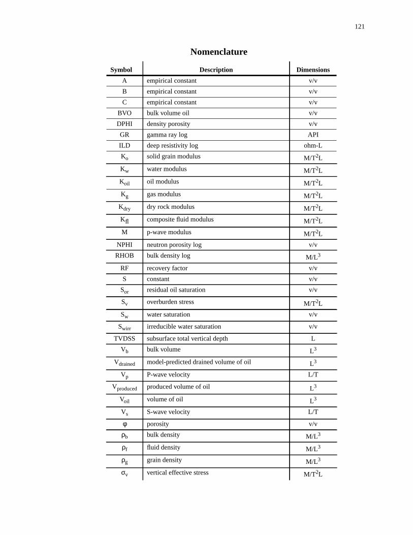
121

Nomenclature

Symbol Description Dimensions

A empirical constant v/v

B empirical constant v/v

C empirical constant v/v

BVO bulk volume oil v/v

DPHI density porosity v/v

GR gamma ray log API

ILD deep resistivity log ohm-L

Ko solid grain modulus M/T2L

Kw water modulus M/T2L

Koil oil modulus M/T2L

Kg gas modulus M/T2L

Kdry dry rock modulus M/T2L

Kfl composite fluid modulus M/T2L

M p-wave modulus M/T2L

NPHI neutron porosity log v/v

RHOB bulk density log M/L3

RF recovery factor v/v

S constant v/v

Sor residual oil saturation v/v

Sv overburden stress M/T2L

Sw water saturation v/v

Swirr irreducible water saturation v/v

TVDSS subsurface total vertical depth L

Vb bulk volume L3

Vdrained model-predicted drained volume of oil L3

Vp P-wave velocity L/T

Vproduced produced volume of oil L3

Voil volume of oil L3

Vs S-wave velocity L/T

φ porosity v/v

ρb bulk density M/L3

ρf fluid density M/L3

ρg grain density M/L3

σv vertical effective stress M/T2L

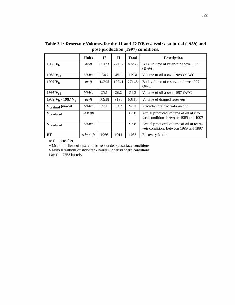
122

ac-ft = acre-feetMMrb = millions of reservoir barrels under subsurface conditionsMMstb = millions of stock tank barrels under standard conditions1 ac-ft = 7758 barrels

Table 3.1: Reservoir Volumes for the J1 and J2 RB reservoirs at initial (1989) andpost-production (1997) conditions.

Units J2 J1 Total Description

1989 Vb ac-ft 65133 22132 87265 Bulk volume of reservoir above 1989OOWC

1989 Voil MMrb 134.7 45.1 179.8 Volume of oil above 1989 OOWC

1997 Vb ac-ft 14205 12941 27146 Bulk volume of reservoir above 1997OWC

1997 Voil MMrb 25.1 26.2 51.3 Volume of oil above 1997 OWC

1989 Vb - 1997 Vb ac-ft 50928 9190 60118 Volume of drained reservoir

Vdrained (model) MMrb 77.1 13.2 90.3 Predicted drained volume of oil

Vproduced MMstb 68.8 Actual produced volume of oil at sur-face conditions between 1989 and 1997

Vproduced MMrb 97.8 Actual produced volume of oil at reser-voir conditions between 1989 and 1997

RF stb/ac-ft 1066 1011 1058 Recovery factor

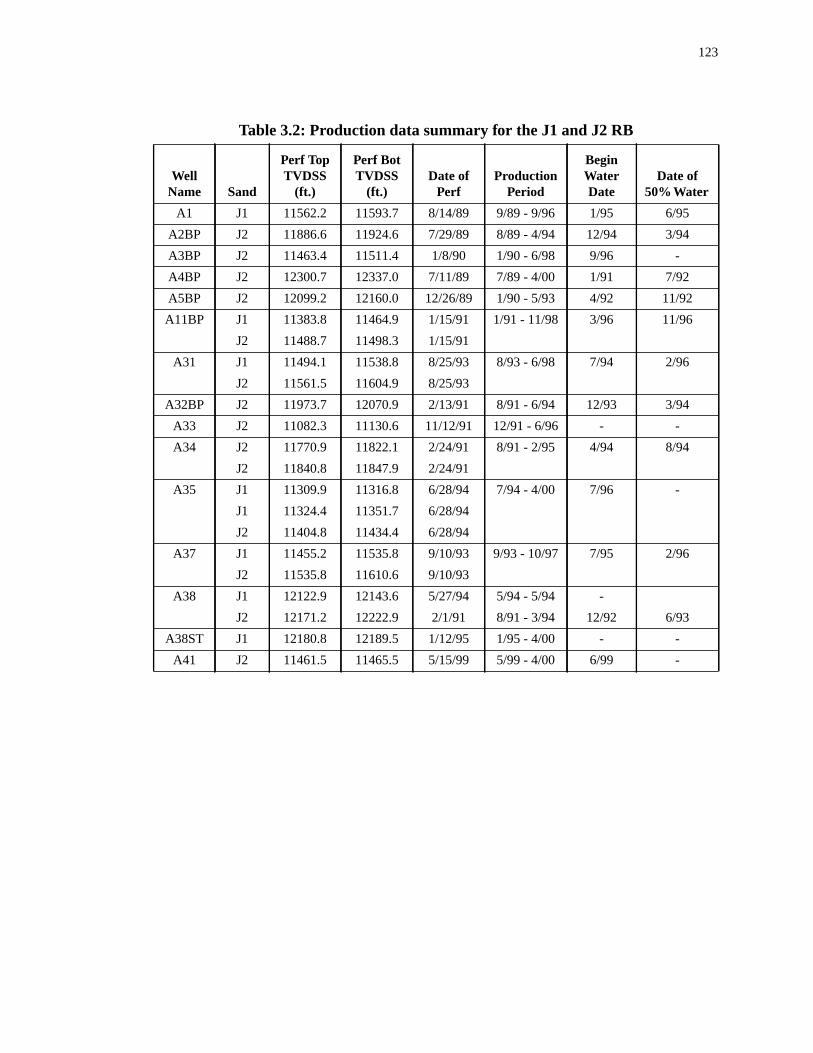
123

Table 3.2: Production data summary for the J1 and J2 RB

WellName Sand

Perf TopTVDSS

(ft.)

Perf BotTVDSS

(ft.)Date of

PerfProduction

Period

BeginWaterDate

Date of50% Water

A1 J1 11562.2 11593.7 8/14/89 9/89 - 9/96 1/95 6/95

A2BP J2 11886.6 11924.6 7/29/89 8/89 - 4/94 12/94 3/94

A3BP J2 11463.4 11511.4 1/8/90 1/90 - 6/98 9/96 -

A4BP J2 12300.7 12337.0 7/11/89 7/89 - 4/00 1/91 7/92

A5BP J2 12099.2 12160.0 12/26/89 1/90 - 5/93 4/92 11/92

A11BP J1 11383.8 11464.9 1/15/91 1/91 - 11/98 3/96 11/96

J2 11488.7 11498.3 1/15/91

A31 J1 11494.1 11538.8 8/25/93 8/93 - 6/98 7/94 2/96

J2 11561.5 11604.9 8/25/93

A32BP J2 11973.7 12070.9 2/13/91 8/91 - 6/94 12/93 3/94

A33 J2 11082.3 11130.6 11/12/91 12/91 - 6/96 - -

A34 J2 11770.9 11822.1 2/24/91 8/91 - 2/95 4/94 8/94

J2 11840.8 11847.9 2/24/91

A35 J1 11309.9 11316.8 6/28/94 7/94 - 4/00 7/96 -

J1 11324.4 11351.7 6/28/94

J2 11404.8 11434.4 6/28/94

A37 J1 11455.2 11535.8 9/10/93 9/93 - 10/97 7/95 2/96

J2 11535.8 11610.6 9/10/93

A38 J1 12122.9 12143.6 5/27/94 5/94 - 5/94 -

J2 12171.2 12222.9 2/1/91 8/91 - 3/94 12/92 6/93

A38ST J1 12180.8 12189.5 1/12/95 1/95 - 4/00 - -

A41 J2 11461.5 11465.5 5/15/99 5/99 - 4/00 6/99 -

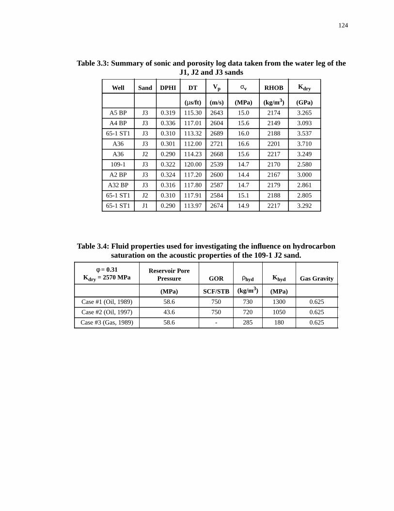
124

Table 3.3: Summary of sonic and porosity log data taken from the water leg of theJ1, J2 and J3 sands

Well Sand DPHI DT Vp σv RHOB Kdry

(µs/ft) (m/s) (MPa) (kg/m3) (GPa)

A5 BP J3 0.319 115.30 2643 15.0 2174 3.265

A4 BP J3 0.336 117.01 2604 15.6 2149 3.093

65-1 ST1 J3 0.310 113.32 2689 16.0 2188 3.537

A36 J3 0.301 112.00 2721 16.6 2201 3.710

A36 J2 0.290 114.23 2668 15.6 2217 3.249

109-1 J3 0.322 120.00 2539 14.7 2170 2.580

A2 BP J3 0.324 117.20 2600 14.4 2167 3.000

A32 BP J3 0.316 117.80 2587 14.7 2179 2.861

65-1 ST1 J2 0.310 117.91 2584 15.1 2188 2.805

65-1 ST1 J1 0.290 113.97 2674 14.9 2217 3.292

Table 3.4: Fluid properties used for investigating the influence on hydrocarbonsaturation on the acoustic properties of the 109-1 J2 sand.

φ = 0.31Kdry = 2570 MPa

Reservoir PorePressure GOR ρhyd Khyd Gas Gravity

(MPa) SCF/STB (kg/m3) (MPa)

Case #1 (Oil, 1989) 58.6 750 730 1300 0.625

Case #2 (Oil, 1997) 43.6 750 720 1050 0.625

Case #3 (Gas, 1989) 58.6 - 285 180 0.625

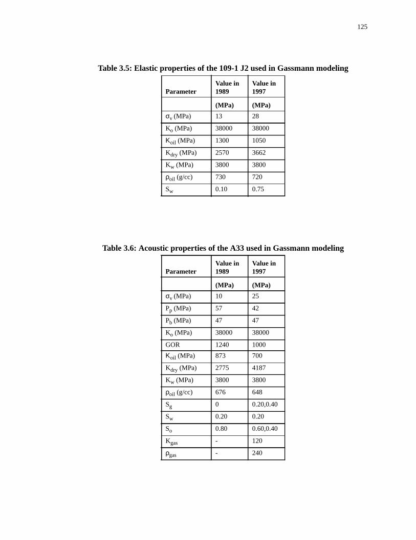
125

Table 3.5: Elastic properties of the 109-1 J2 used in Gassmann modeling

ParameterValue in1989

Value in1997

(MPa) (MPa)

σv (MPa) 13 28

Ko (MPa) 38000 38000

Κoil (MPa) 1300 1050

Kdry (MPa) 2570 3662

Kw (MPa) 3800 3800

ρoil (g/cc) 730 720

Sw 0.10 0.75

Table 3.6: Acoustic properties of the A33 used in Gassmann modeling

ParameterValue in1989

Value in1997

(MPa) (MPa)

σv (MPa) 10 25

Pp (MPa) 57 42

Pb (MPa) 47 47

Ko (MPa) 38000 38000

GOR 1240 1000

Κoil (MPa) 873 700

Kdry (MPa) 2775 4187

Kw (MPa) 3800 3800

ρoil (g/cc) 676 648

Sg 0 0.20,0.40

Sw 0.20 0.20

So 0.80 0.60,0.40

Kgas - 120

ρgas - 240

126

nic

oni-ld:

lus,id-

ser-65,

is,

ringre

re,

ng

of

nts:

References

Alberty, M., 1996, The influence of the borehole environment upon compressional sologs:The Log Analyst, vol. 37 no. 4, pp. 30 - 45.

Batzle, M. and Wang, Z., 1992, Seismic properties of pore fluids:Geophysics, vol. 57 no.11, pp1396 - 1408.

Behrens, R., Condon, P., Haworth, W., Bergeron, M., Wang, Z., 2001, 4D seismic mtoring of water influx at Bay Marchand: the practical use of 4D in an imperfect worSPE 71329.

Benson, A.K., and Wu, J., 1999, A modeling solution for predicting a) dry rock modurigidity modulus and b) seismic velocities and reflection coefficients in porous, flufilled rocks with applications to rock samples and well logs:Journal of Applied Geo-physics, vol. 41, pp. 49 - 73.

Berryman, J.G., Origin of Gassmann’s equations: Geophysics, vol. 64 no. 5, pp. 1627 -1629.

Best, K.D., 2002, Development of an integrated model for compaction/water drive revoirs and its application to the J1 and J2 Sand at Bullwinkle, Green Canyon BlockGulf of Mexico: Masters thesis, The Pennsylvania State University.

Blangy, J.P., 1992, Integrated seismic lithologic interpretation: the petrophysical basStanford University Phd thesis, 414 pp.

Burkhart, T., Hoover, A.R., and Flemings, P.B., 1998, Time-lapse (4D) seismic monitoof primary production of turbidite reservoirs at South Timbalier Block 295, offshoLouisiana, Gulf of Mexico:Geophysics, vol. 65 no. 2, pp. 351 - 367.

Burkhart, T, 1997, Time lapse monitoring of the South Timbalier block 295 field, offshoLouisiana: Masters these, The Pennsylvania State University.

Christensen, N.I., and Wang, H.F., 1985, The influence of pore pressure and confinipressure on dynamic elastic properties of Berea sandstone: Geophysics, vol. 50 no. 2,pp. 207-213.

Clark, V.A., 1992, The effect of oil under in-situ conditions on the seismic propertiesrocks:Geophysics, vol.57 no. 7, pp. 894 - 901.

Domenico N., 1977, Elastic properties of unconsolidated porous sand reservoirs:Geo-physics, vol. 42 no. 7, pp. 1339 - 1368.

Dvorkin, J., Prasad, M., Sakai, A., and Lavoie, D., 1998, Elasticity of marine sedimeJournal of Geophysical Research, vol. 26, pp. 1781 - 1784.

127

ong

in

dia):

tary

por-to

m

ks

V

ela-

at-

g

dated

Eberhart-Phillips, D., Han, D-H., and Zoback, M.D., 1989, Empirical relationships amseismic velocity, effective pressure, porosity, and clay content in sandstone:Geophys-ics, vol. 54, no. 1, pp. 82 - 89.


Gassmann, F., 1951, Elastic waves through a packing of spheres:Geophysics, vol.16 pp.673 - 685.

Gassmann, F., 1951, Uber die Elastizitat poroser Medien (On elasticity of porous meVeirteljahrsschrift der Naturforschenden Gesellschaft in Zurich, 96, pp. 1-23.

Gregory, A.R., 1976, Fluid saturation effects on dynamic elastic properties of sedimenrocks:Geophysics, vol 41, pp. 895 - 921.

Gregory, A.R., 1977, Aspects of rock physics from laboratory and log data that are imtant t seismic interpretationin Payton, C.E. (Ed.), Seismic-stratigraphy applicationhydrocarbon exploration, vol. 26, AAPG Memoir, pp. 15-46.

Han, D., Nur, A., and Morgan, D., 1986, Effects of porosity and clay content on wavevelocities in sandstones:Geophysics, vol. 51., pp. 2093 - 2107.

Landro, M., 2001, Discrimination between pressure and fluid saturation changes frotime lapse seismic data:Geophysics, vol. 66, no. 3, pp. 836 - 844.

Landro, M., Solheim, O.A., Hilde, E., Ekren, B.O., and Stronen, L.K., 1999, The Gulfa4D seismic study:Petroleum Geoscience, vol 5, pp. 213 - 226.

Mavko, G., Chan, C., and Mukerji, T., 1995, Fluid substitution: estimating changes inpwithout knowing Vs:Geophysics, vol. 60 no. 6, pp. 1750 - 1755.

Mavko, G., Mukerji, T., 1995, Seismic pore space compressibility and Gassmann’s rtion: Geophysics, vol. 60 no. 6, pp. 1743 - 1749.

Nur, A., Mavko, G., Dvorkin, J., and Galmudi, D., 1998, Critical porosity: A key to reling physical properties to porosity in rocks:The Leading Edge, vol. 17, pp. 357-362.

Packwood, J.L., 1996, Feasibility of hydrocarbon recovery monitoring with increasinrock frame stiffness: SEG Expanded Abstract, pp. 876 - 878.

Spencer, J.W., Cates, M.E., and Thompson, D.D., 1994, Frame moduli of unconsolisands and sandstones,Geophysics, vol. 59 no. 9, pp. 1352 - 1361.

128

salin-

nal

ero-

el:

s on

ffec-

Jones, S.M., McCann, C., Astin, R., and Sothcott, J., 1988, The effects of pore-fluidity on ultrasonic wave propagation in sandstones:Geophysics, vol. 63 no. 3, pp. 928 -934.

Murphy, W., Reischer, A., and Hsu, K., 1993, Modulus decomposition of compressioand shear velocities in sand bodies:Geophysics vol. 58 no. 2, pp. 227 - 239.

Wyllie, M.R.J., Gregory, A.R., and Gardner, L.W., 1956, Elastic wave velocities in hetgeneous and porous media:Geophysicsvol. 21 no. 1, pp. 41 - 70.

Fanchi, J.R., 1999, Predicting 4D seismic performance using an integrated flow modSPE Annual Technical Conference and Exhibition, SPE 56527.

Whitman, W.W., and Towle, G.H., 1992, The influence of elastic and density propertiethe behavior of the Gassmann relation:The Log Analyst, vol.33, no.6, pp.500-506.

Wang, Z., 2001, Fundamentals of seismic rock physics:Geophysics, vol. 66 no. 2, pp. 398- 412.

Zhang, J.J., and Bentley, L.R., 2000, Change of elastic moduli of dry sandstone with etive pressure. SEG Expanded Abstract.

129

y are

ent

ns

ei of

ation

,

al to

al

igher

sity

e

Appendix A - PNC Log Methodology

PNC logs are useful tools for investigating water saturation changes because the

most sensitive to the presence of NaCl in formation water. The PNC log measurem

used to determine Sw is based on the ability of the formation to capture thermal neutro

emitted by the tool sonde (Smolen, 1996) and is called the cross-section (Σ). When high-

energy thermal neutrons are introduced into the formation, they interact with the nucl

different formation materials. These nuclear interactions or captures result in the cre

of a gamma-ray which is measured by a counter in the tool (Bateman, 1984; Smolen

1996). The rate at which thermal neutrons are captured by the formation is proportion

its cross-section or sigma. A formation with a given porosity will capture more therm

neutrons when it is 100% water saturated, so the sigma value recorded by the tool is h

than in an oil-filled formation with the same porosity.

I use a volume-average approach for calculating Sw from PNC logs. The simple for-

mation model includes sigma responses from the solid grains, and the effective poro

filled with water and hydrocarbon,

. (A.1)

Using the porosity from the bulk density log, Sw was calculated by rearranging the abov

equation to:

(A.2)

Σ 1 φ–( )Σm φ 1 Sw–( )Σh φSwΣw+ +=

Sw

Σ Σm–( ) φ Σh Σm–( )–

φ Σw Σh–( )------------------------------------------------------=

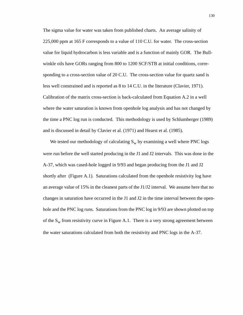
130

ion

ull-

-

d is

.

l

d by

989)

n the

ave

hat no

open-

n top

een

The sigma value for water was taken from published charts. An average salinity of

225,000 ppm at 165 F corresponds to a value of 110 C.U. for water. The cross-sect

value for liquid hydrocarbon is less variable and is a function of mainly GOR. The B

winkle oils have GORs ranging from 800 to 1200 SCF/STB at initial conditions, corre

sponding to a cross-section value of 20 C.U. The cross-section value for quartz san

less well constrained and is reported as 8 to 14 C.U. in the literature (Clavier, 1971)

Calibration of the matrix cross-section is back-calculated from Equation A.2 in a wel

where the water saturation is known from openhole log analysis and has not change

the time a PNC log run is conducted. This methodology is used by Schlumberger (1

and is discussed in detail by Clavier et al. (1971) and Hearst et al. (1985).

We tested our methodology of calculating Sw by examining a well where PNC logs

were run before the well started producing in the J1 and J2 intervals. This was done i

A-37, which was cased-hole logged in 9/93 and began producing from the J1 and J2

shortly after (Figure A.1). Saturations calculated from the openhole resistivity log h

an average value of 15% in the cleanest parts of the J1/J2 interval. We assume here t

changes in saturation have occurred in the J1 and J2 in the time interval between the

hole and the PNC log runs. Saturations from the PNC log in 9/93 are shown plotted o

of the Sw from resistivity curve in Figure A.1. There is a very strong agreement betw

the water saturations calculated from both the resistivity and PNC logs in the A-37.

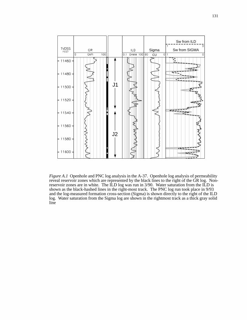
131

ilityNon- is/93ILDolid

Figure A.1 Openhole and PNC log analysis in the A-37. Openhole log analysis of permeabreveal reservoir zones which are represented by the black lines to the right of the GR log.reservoir zones are in white. The ILD log was run in 3/90. Water saturation from the ILDshown as the black-hashed lines in the right-most track. The PNC log run took place in 9and the log-measured formation cross-section (Sigma) is shown directly to the right of thelog. Water saturation from the Sigma log are shown in the rightmost track as a thick gray sline

J1

J2

Sw from ILD

Sw from SIGMASigmaCU

132

g

ring:

eu-

eu-apse

References

Smolen, J.J., 1996, Cased Hole and Production Log Evaluation: Penn Well PublishinCompany, 365 p.

Bateman, R.M., 1985, Cased-Hole Log Analysis and Reservoir Performance MonitoInternational Human Resources Development Corporation, 319 p.

Clavier, C, Hoyle, W., and Meunier, D., 1971, Quantitative interpretation of thermal ntron decay logs, Part I: Fundamentals and techniques,Journal of Petroleum Technol-ogy, vol. 23, June, pp. 743-755.

Clavier, C, Hoyle, W., and Meunier, D., 1971, Quantitative interpretation of thermal ntron decay logs, Part II: Interpretation example, interpretation accuracy, and time-ltechnique, Journal of Petroleum Technology, vol. 23, June, pp. 743-755.

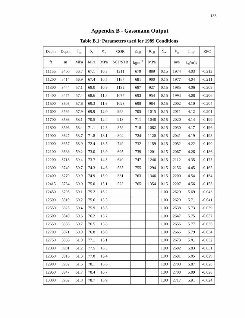
133

2

1

9

6

4

1

9

6

3

0

6

5

5

4

3

Appendix B - Gassmann Output

Table B.1: Parameters used for 1989 Conditions

Depth Depth Pp Sv σv GOR ρoil Koil Sw Vp Imp RFC

ft m MPa MPa MPa SCF/STB kg/m3 MPa m/s kg/m2s

11155 3400 56.7 67.1 10.3 1211 679 889 0.15 1974 4.03 -0.21

11200 3414 56.9 67.4 10.5 1187 681 900 0.15 1977 4.04 -0.21

11300 3444 57.1 68.0 10.9 1132 687 927 0.15 1985 4.06 -0.20

11400 3475 57.4 68.6 11.3 1077 693 954 0.15 1993 4.08 -0.20

11500 3505 57.6 69.3 11.6 1023 698 984 0.15 2002 4.10 -0.20

11600 3536 57.9 69.9 12.0 968 705 1015 0.15 2011 4.12 -0.20

11700 3566 58.1 70.5 12.4 913 711 1048 0.15 2020 4.14 -0.19

11800 3596 58.4 71.1 12.8 859 718 1082 0.15 2030 4.17 -0.19

11900 3627 58.7 71.8 13.1 804 724 1120 0.15 2041 4.19 -0.19

12000 3657 58.9 72.4 13.5 749 732 1159 0.15 2052 4.22 -0.19

12100 3688 59.2 73.0 13.9 695 739 1201 0.15 2067 4.26 -0.18

12200 3718 59.4 73.7 14.3 640 747 1246 0.15 2112 4.35 -0.17

12300 3749 59.7 74.3 14.6 585 755 1294 0.15 2156 4.45 -0.16

12400 3779 59.9 74.9 15.0 531 763 1346 0.15 2200 4.54 -0.15

12415 3784 60.0 75.0 15.1 523 765 1354 0.15 2207 4.56 -0.15

12450 3795 60.1 75.2 15.2 1.00 2620 5.69 -0.043

12500 3810 60.2 75.6 15.3 1.00 2629 5.71 -0.041

12550 3825 60.4 75.9 15.5 1.00 2638 5.73 -0.039

12600 3840 60.5 76.2 15.7 1.00 2647 5.75 -0.037

12650 3856 60.7 76.5 15.8 1.00 2656 5.77 -0.036

12700 3871 60.9 76.8 16.0 1.00 2665 5.79 -0.034

12750 3886 61.0 77.1 16.1 1.00 2673 5.81 -0.032

12800 3901 61.2 77.5 16.3 1.00 2682 5.83 -0.031

12850 3916 61.3 77.8 16.4 1.00 2691 5.85 -0.029

12900 3932 61.5 78.1 16.6 1.00 2700 5.87 -0.028

12950 3947 61.7 78.4 16.7 1.00 2708 5.89 -0.026

13000 3962 61.8 78.7 16.9 1.00 2717 5.91 -0.024

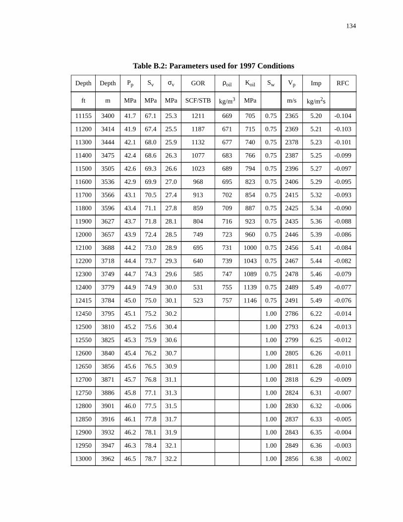
134

4

3

1

9

7

5

3

0

8

6

4

2

9

7

6

Table B.2: Parameters used for 1997 Conditions

Depth Depth Pp Sv σv GOR ρoil Koil Sw Vp Imp RFC

ft m MPa MPa MPa SCF/STB kg/m3 MPa m/s kg/m2s

11155 3400 41.7 67.1 25.3 1211 669 705 0.75 2365 5.20 -0.10

11200 3414 41.9 67.4 25.5 1187 671 715 0.75 2369 5.21 -0.10

11300 3444 42.1 68.0 25.9 1132 677 740 0.75 2378 5.23 -0.10

11400 3475 42.4 68.6 26.3 1077 683 766 0.75 2387 5.25 -0.09

11500 3505 42.6 69.3 26.6 1023 689 794 0.75 2396 5.27 -0.09

11600 3536 42.9 69.9 27.0 968 695 823 0.75 2406 5.29 -0.09

11700 3566 43.1 70.5 27.4 913 702 854 0.75 2415 5.32 -0.09

11800 3596 43.4 71.1 27.8 859 709 887 0.75 2425 5.34 -0.09

11900 3627 43.7 71.8 28.1 804 716 923 0.75 2435 5.36 -0.08

12000 3657 43.9 72.4 28.5 749 723 960 0.75 2446 5.39 -0.08

12100 3688 44.2 73.0 28.9 695 731 1000 0.75 2456 5.41 -0.08

12200 3718 44.4 73.7 29.3 640 739 1043 0.75 2467 5.44 -0.08

12300 3749 44.7 74.3 29.6 585 747 1089 0.75 2478 5.46 -0.07

12400 3779 44.9 74.9 30.0 531 755 1139 0.75 2489 5.49 -0.07

12415 3784 45.0 75.0 30.1 523 757 1146 0.75 2491 5.49 -0.07

12450 3795 45.1 75.2 30.2 1.00 2786 6.22 -0.014

12500 3810 45.2 75.6 30.4 1.00 2793 6.24 -0.013

12550 3825 45.3 75.9 30.6 1.00 2799 6.25 -0.012

12600 3840 45.4 76.2 30.7 1.00 2805 6.26 -0.011

12650 3856 45.6 76.5 30.9 1.00 2811 6.28 -0.010

12700 3871 45.7 76.8 31.1 1.00 2818 6.29 -0.009

12750 3886 45.8 77.1 31.3 1.00 2824 6.31 -0.007

12800 3901 46.0 77.5 31.5 1.00 2830 6.32 -0.006

12850 3916 46.1 77.8 31.7 1.00 2837 6.33 -0.005

12900 3932 46.2 78.1 31.9 1.00 2843 6.35 -0.004

12950 3947 46.3 78.4 32.1 1.00 2849 6.36 -0.003

13000 3962 46.5 78.7 32.2 1.00 2856 6.38 -0.002

petrophysical analysis and geologic model for the bullwinkle j sands ...

Documents

Transcript of petrophysical analysis and geologic model for the bullwinkle j sands ...