Yannick PontyLaboratoire Lagrange CNRS

Observatoire de la Côte d'Azur University of the Côte d'Azur (UCA)

          Periodic box simulations and tools

Do we need complex geometry ?

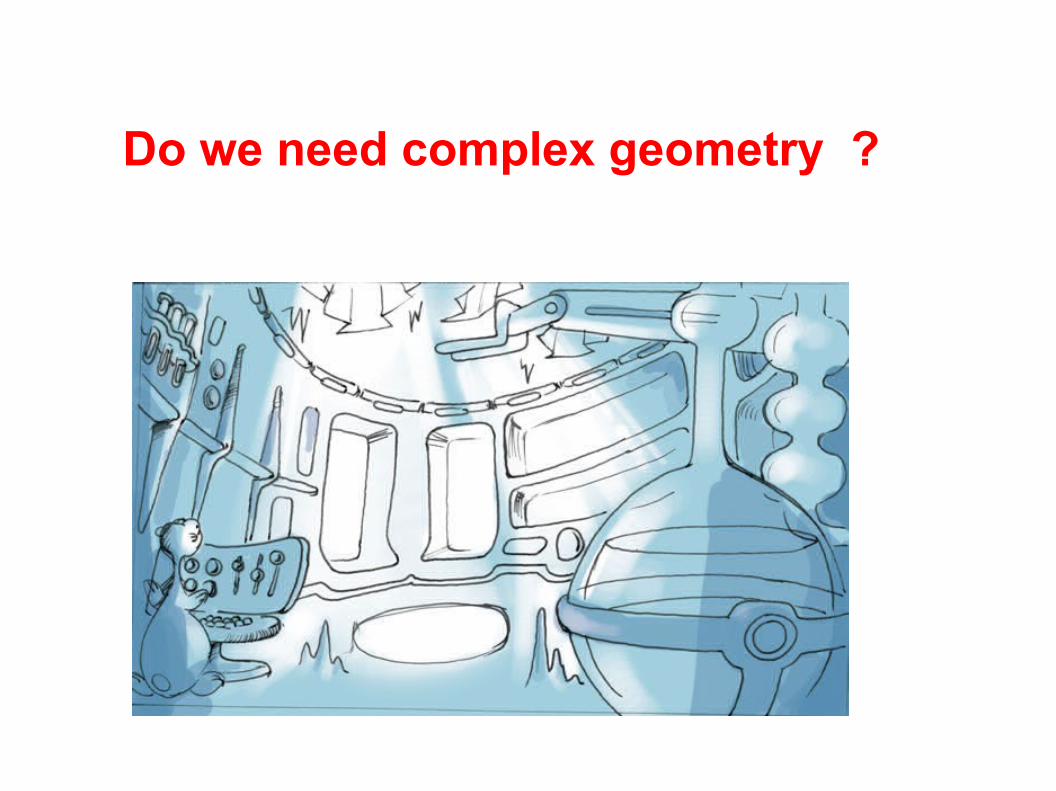
periodic box 2π ³

Let's go inside the 

Outline            Numerical method     (How make a cube yourself : The unrevealed story ! ) 

1) The periodic box a numerical experiment      Fundamental equation, Basic non dimensional number       Pressure, projector , Numerical schema     Parallelization procedure,  Different forcing     tracers 2)  Numerical quantities output and experimental observable       Probe, time signal       Mean flow      3D visualization3) LES,  energy transfer

4)  Penalization method

7

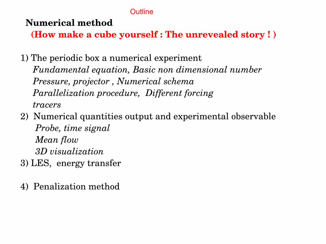
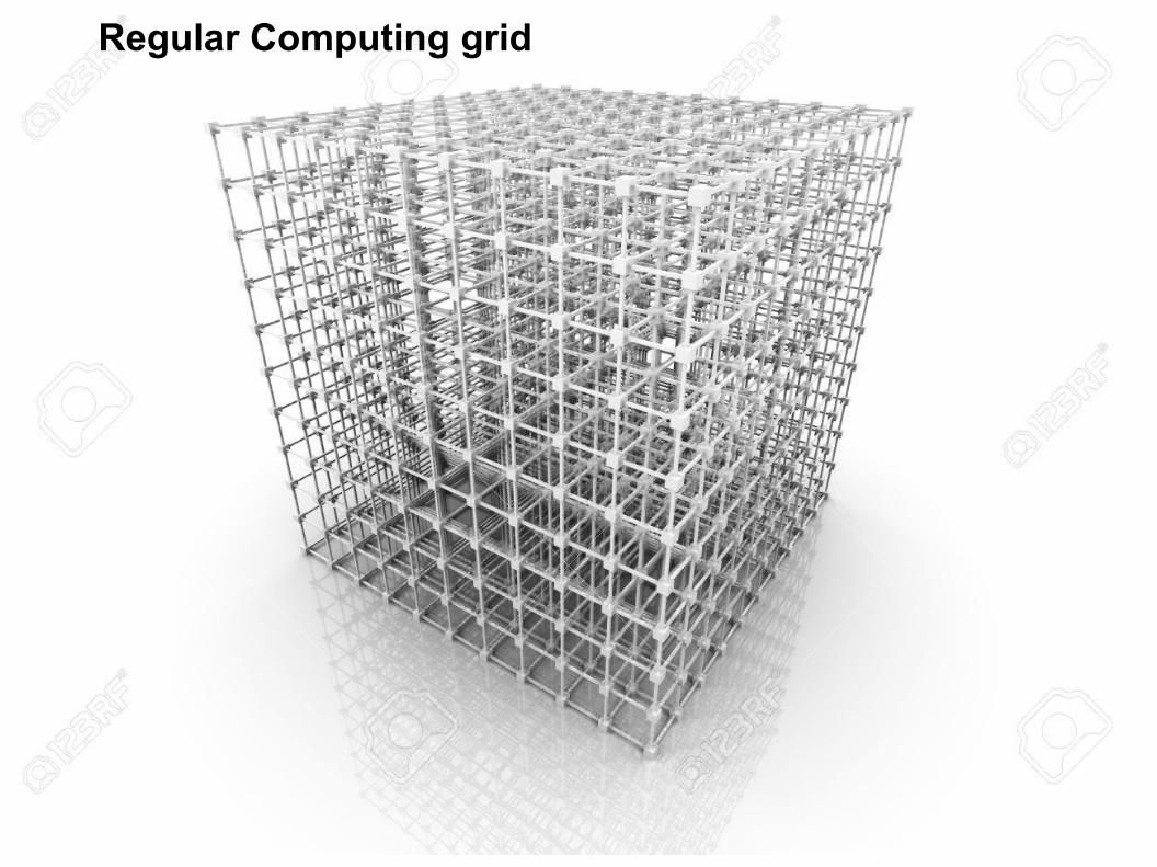
Regular Computing grid

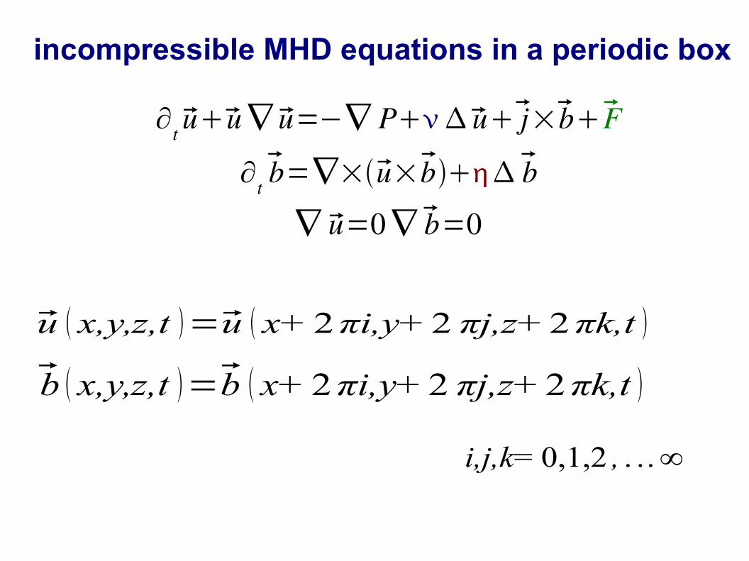
incompressible MHD equations in a periodic box

b x,y,z,t =b x+2πi,y+2 πj,z+2πk,t

u x,y,z,t =u x+2πi,y+2 πj,z+2πk,t

i,j,k= 0,1,2 , . ..∞

∂t uu ∇ u=−∇ P uj×bF

∂tb=∇×u×b b

∇ u=0 ∇ b=0

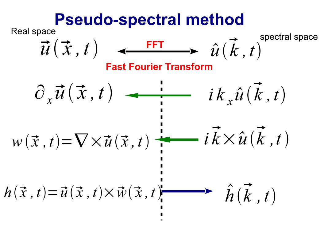
Pseudo-spectral method

∂ xu x , t

u k , t FFT

Fast Fourier Transform

Real spacespectral space

i k x u k , t

u x , t

h x , t =u x , t ×wx , t h k , t

w x , t =∇×u x , t i k×u k ,t

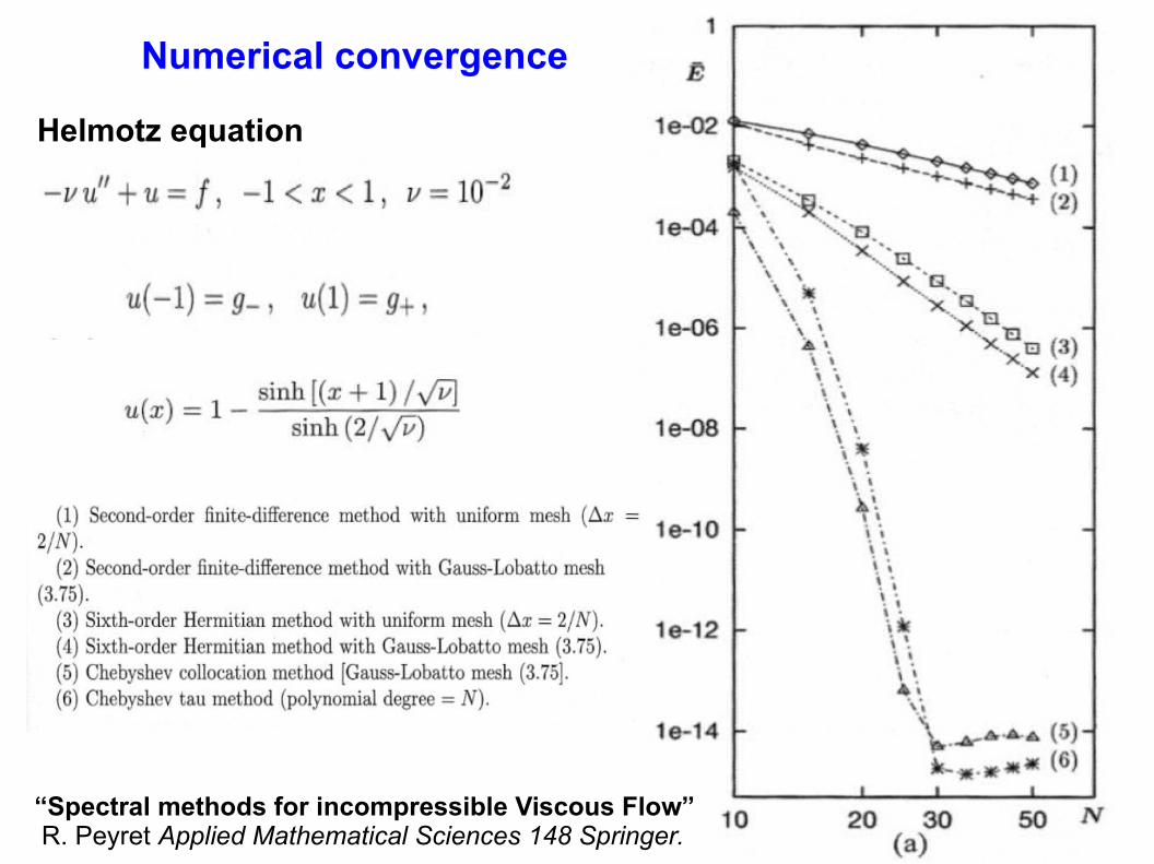
“Spectral methods for incompressible Viscous Flow” R. Peyret Applied Mathematical Sciences 148 Springer.

Helmotz equation

Numerical convergence

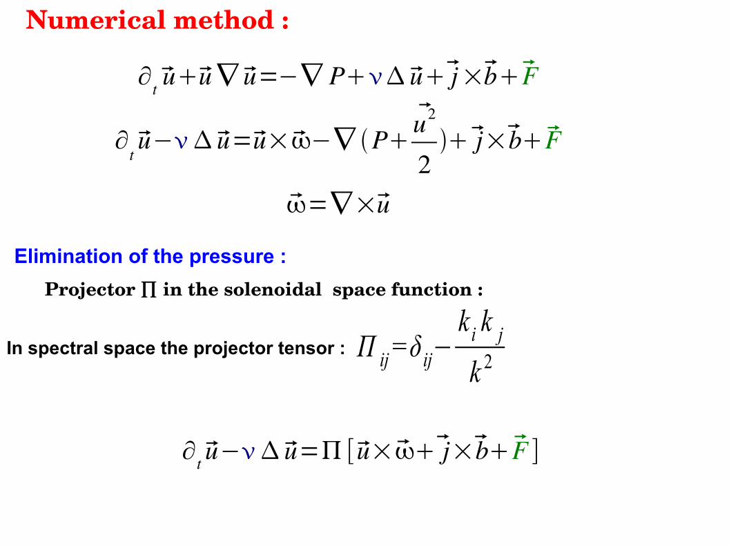
Numerical method :  

Projector ∏ in the solenoidal  space function :  

Elimination of the pressure :

In spectral space the projector tensor : Π ij=δij−k i k j

k 2

∂t uu ∇ u=−∇ P uj ×bF

∂tu− u=u×−∇ P

u2

2j×bF

=∇×u

∂t u− u=[u×j×bF ]

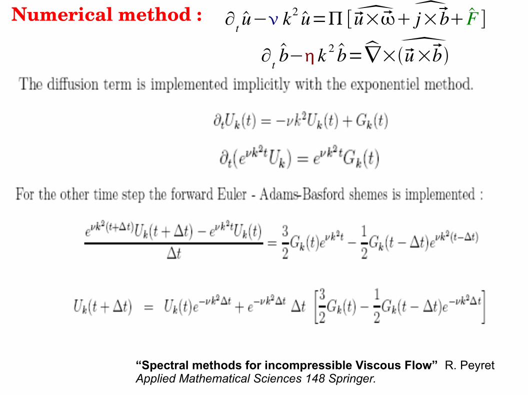
Numerical method :  

“Spectral methods for incompressible Viscous Flow” R. Peyret Applied Mathematical Sciences 148 Springer.

∂tu− k2 u=[u×

j×b F ]

∂tb− k 2 b=∇×

u×b

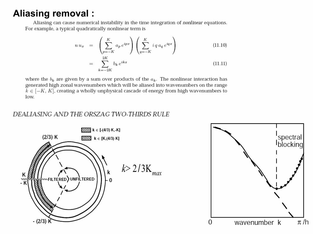
Aliasing removal :

k>2 /3Kmax

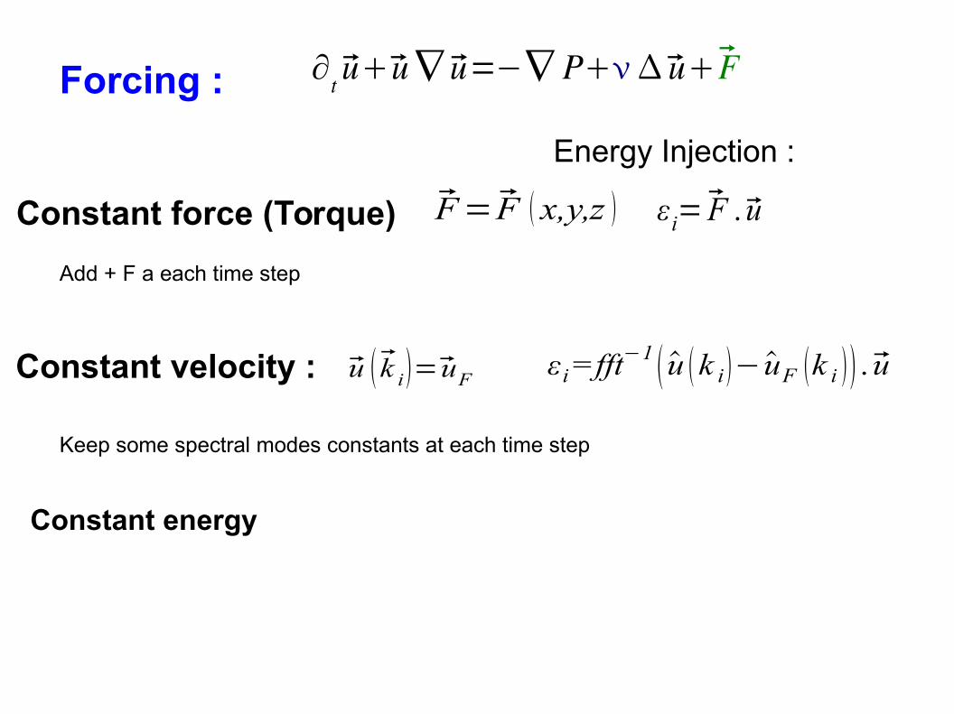
Forcing :

Constant force (Torque)

Constant velocity :

Energy Injection :

F=F x,y,z εi=F .u

u k i =uF

Add + F a each time step

Keep some spectral modes constants at each time step

εi=fft−1 u k i −uF k i .u

∂t uu ∇ u=−∇ P uF

Constant energy

Large eddy simulation (LES) : Large eddy simulation (LES) :

l νkc

ε

ε Control the transfer into the subgrid scale

Ref: “Turbulence in Fluids” M. Lesieur Kluwer “Large Eddy Simulation for incompressible flow” P. Sagaut Springer

J.P Chollet & M. Lesieur J. Admos. Sci 38 (1981)

ν k,t =0 . 441C k

32 E K c−no ,t

K c−no

H k

Kc -no

Cups function

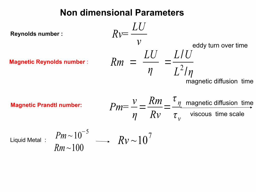
Non dimensional Parameters

Magnetic Reynolds number :

Reynolds number :

Magnetic Prandtl number:

Rv=LUν

Rm =LUη

=L /U

L2 /η

eddy turn over time

magnetic diffusion time

Pm=νη=

RmRv

=τ ητν

Liquid Metal :Pm ~ 10−5

Rm ~100Rv ~107

magnetic diffusion time

viscous time scale

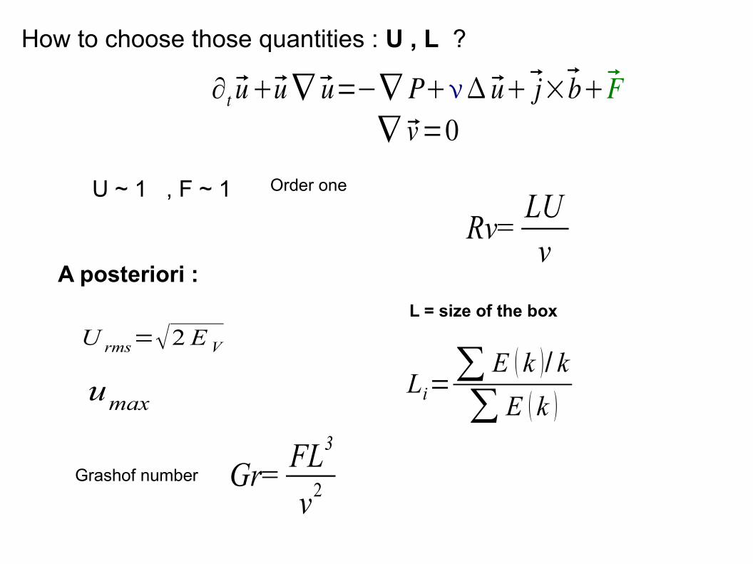
How to choose those quantities : U , L ?

A posteriori :

U rms=√2 E V

Li=∑ E k / k

∑ E k

L = size of the box

∂t uu ∇ u=−∇ P uj×bF∇ v=0

umax

U ~ 1 , F ~ 1 Order one

Rv=LUν

Grashof number Gr=FL3

ν2

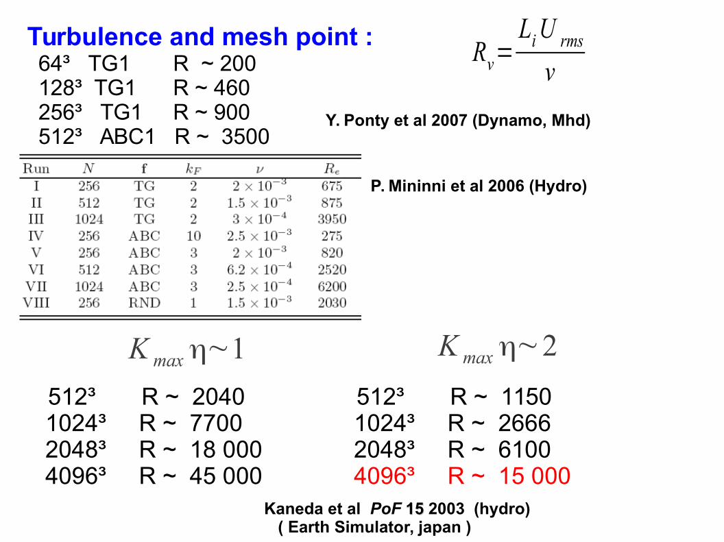
Turbulence and mesh point : 64³ TG1 R ~ 200 128³ TG1 R ~ 460 256³ TG1 R ~ 900512³ ABC1 R ~ 3500

Rν=LiU rms

ν

Y. Ponty et al 2007 (Dynamo, Mhd)

P. Mininni et al 2006 (Hydro)

512³ R ~ 2040 1024³ R ~ 7700 2048³ R ~ 18 000 4096³ R ~ 45 000

Kaneda et al PoF 15 15 2003 (hydro) ( Earth Simulator, japan )

K max η∼1 K max η∼2

512³ R ~ 1150 1024³ R ~ 2666 2048³ R ~ 6100 4096³ R ~ 15 000

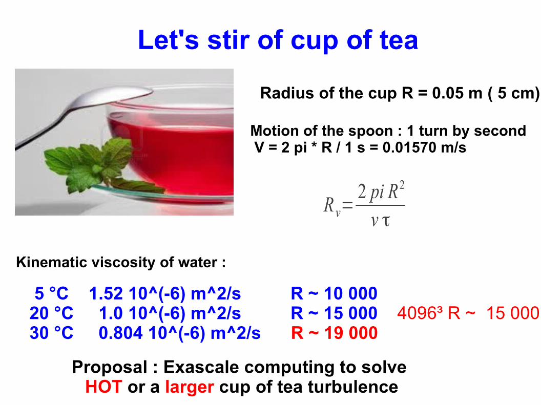
Let's stir of cup of tea

Rν=2 pi R2

ν τ

Radius of the cup R = 0.05 m ( 5 cm)

Motion of the spoon : 1 turn by second V = 2 pi * R / 1 s = 0.01570 m/s

Kinematic viscosity of water :

5 °C 1.52 10^(-6) m^2/s R ~ 10 000 20 °C 1.0 10^(-6) m^2/s R ~ 15 00030 °C 0.804 10^(-6) m^2/s R ~ 19 000

Proposal : Exascale computing to solve HOT or a larger cup of tea turbulence

4096³ R ~ 15 000

20

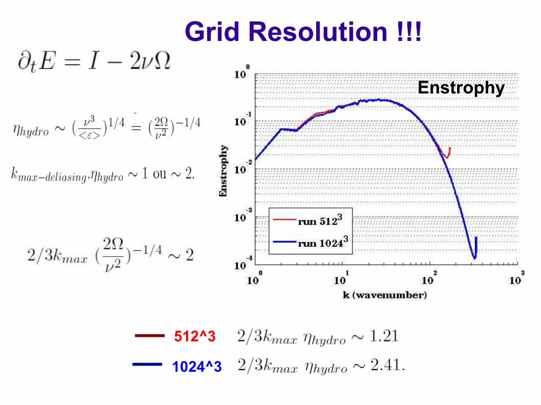
512^3

1024^3

Enstrophy

Grid Resolution !!!

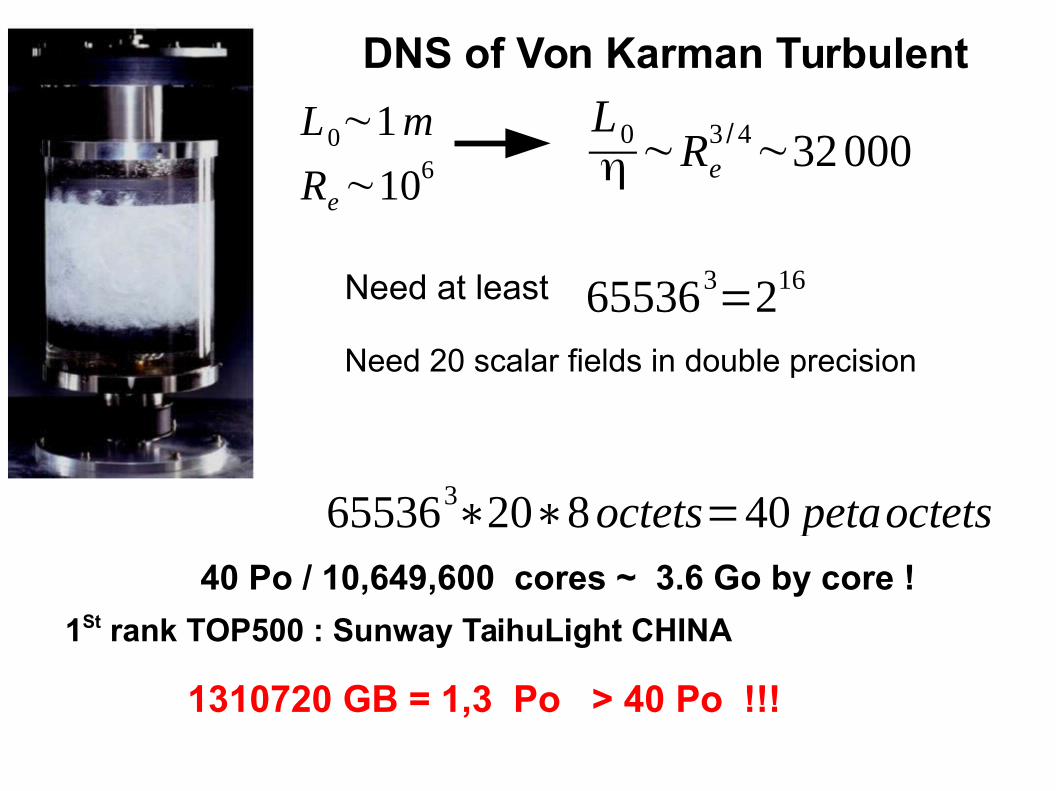
L0η ∼Re

3 /4∼32000

L0∼1m

Re∼106

Need at least 655363=216

Need 20 scalar fields in double precision

655363∗20∗8octets=40 petaoctets

40 Po / 10,649,600 cores ~ 3.6 Go by core !

DNS of Von Karman Turbulent

1St rank TOP500 : Sunway TaihuLight CHINA

1310720 GB = 1,3 Po > 40 Po !!!

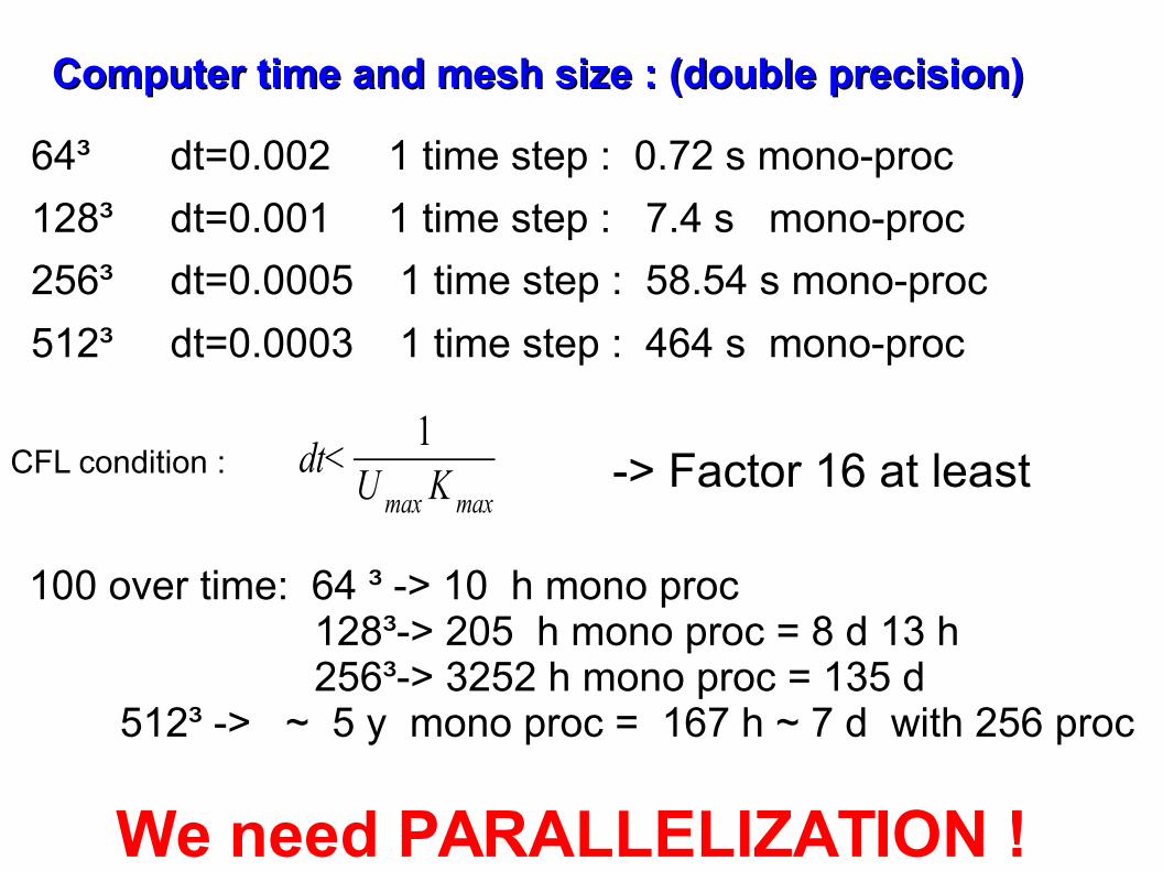
Computer time and mesh size : (double precision) Computer time and mesh size : (double precision)

64³ dt=0.002 1 time step : 0.72 s mono-proc

128³ dt=0.001 1 time step : 7.4 s mono-proc

256³ dt=0.0005 1 time step : 58.54 s mono-proc

512³ dt=0.0003 1 time step : 464 s mono-proc

-> Factor 16 at least

100 over time: 64 ³ -> 10 h mono proc 128³-> 205 h mono proc = 8 d 13 h 256³-> 3252 h mono proc = 135 d 512³ -> ~ 5 y mono proc = 167 h ~ 7 d with 256 proc

CFL condition : dt<1

U max K max

We need PARALLELIZATION !

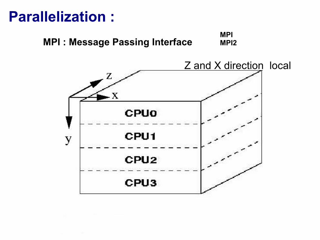
Parallelization :

MPI : Message Passing Interface MPI MPI2

Z and X direction local

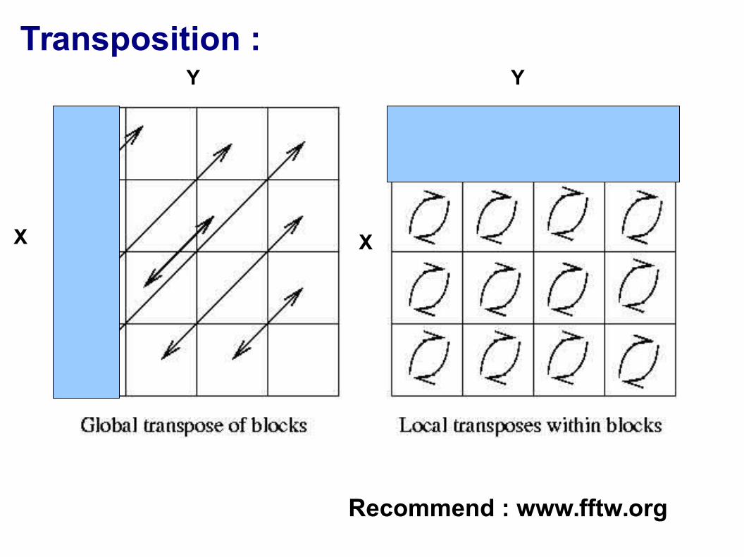
Transposition :

X

Y Y

X

Recommend : www.fftw.org

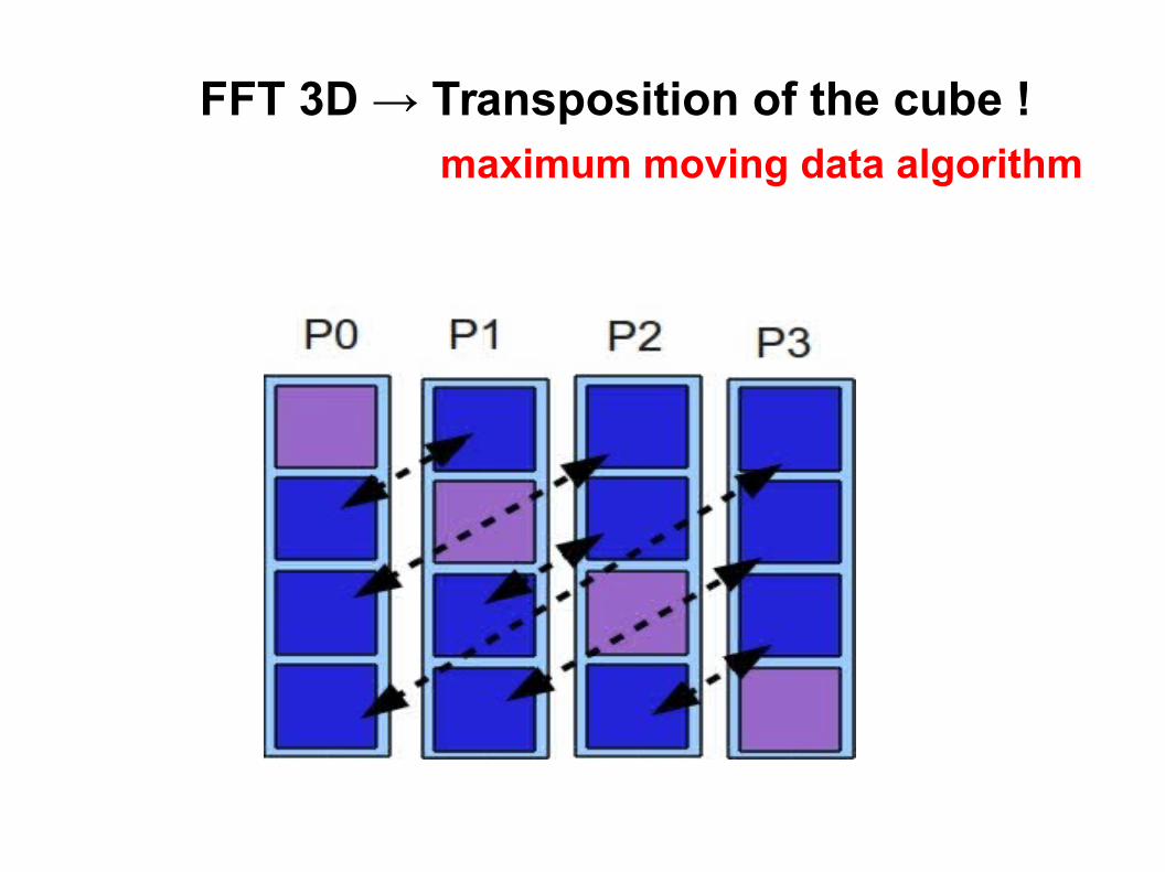
FFT 3D → Transposition of the cube ! maximum moving data algorithm

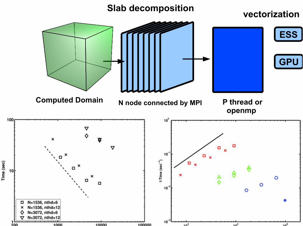
N node connected by MPI P thread or openmp

Computed Domain

Code MIRA (P. Mininni )

Slab decomposition

GPU

ESS

vectorization

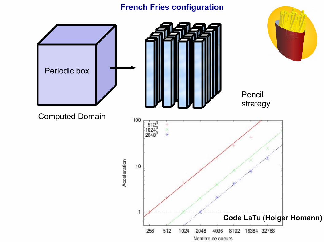
Periodic box

Computed Domain

Pencil strategy

French Fries configuration

Code LaTu (Holger Homann)

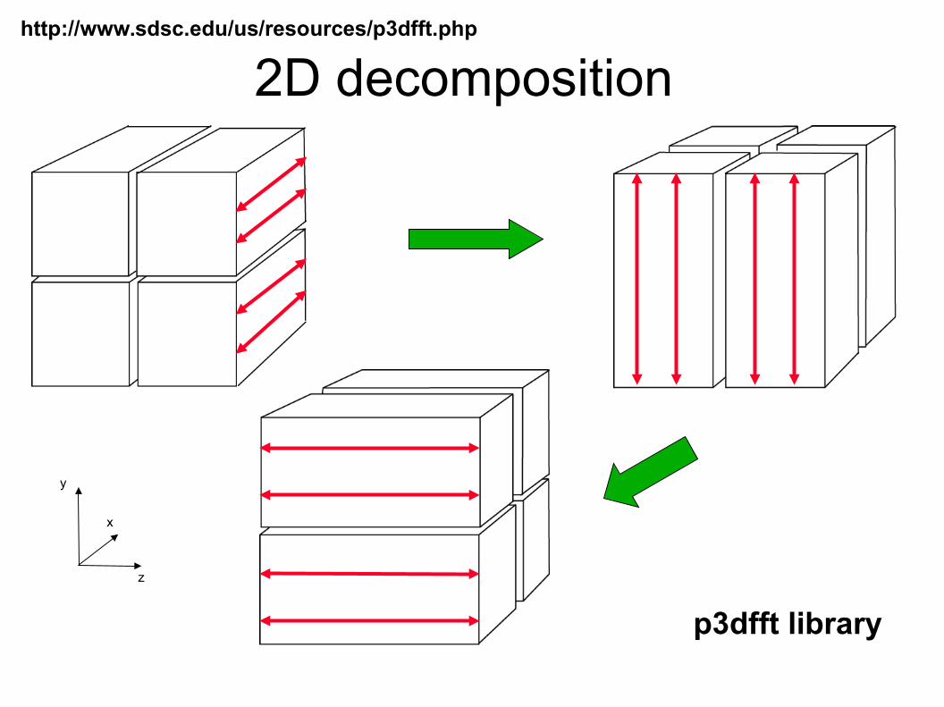
2D decomposition

y

z

x

http://www.sdsc.edu/us/resources/p3dfft.php

p3dfft library

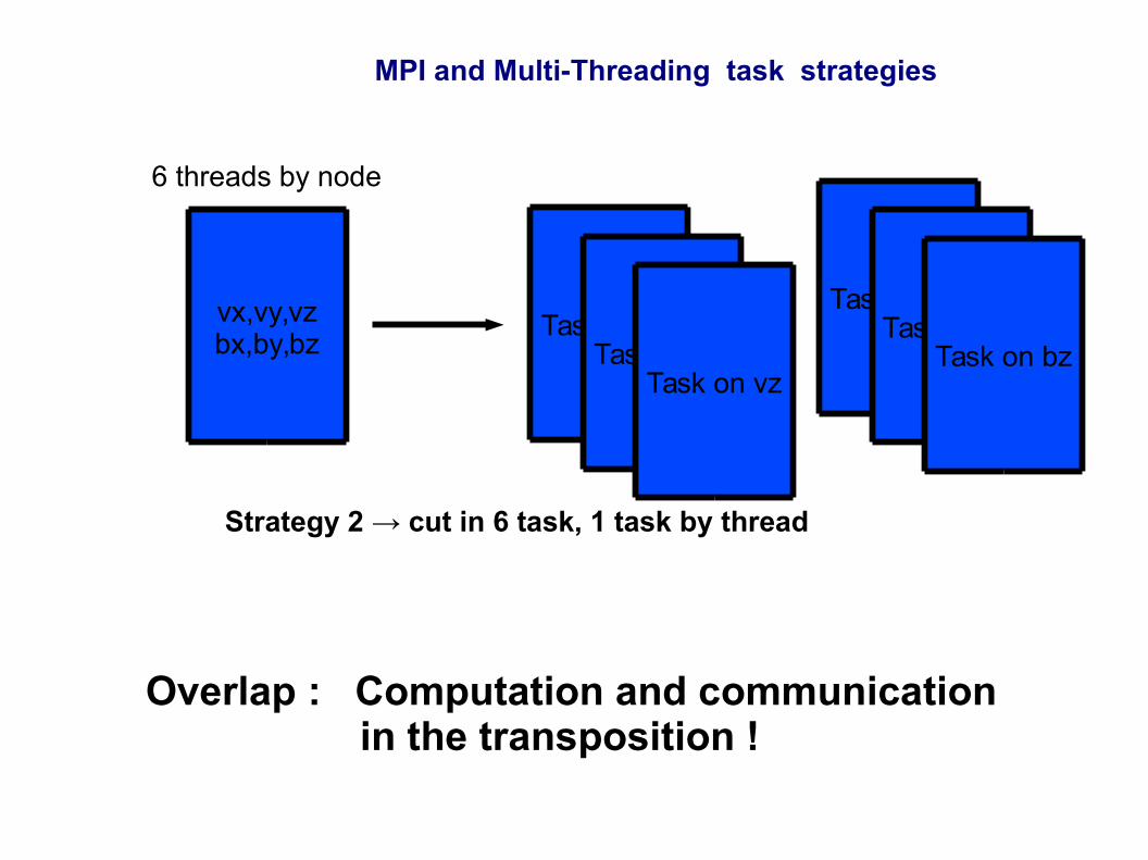
vx,vy,vzbx,by,bz

6 threads by node

Task on vxTask on vy

Task on vz

Task on bxTask on by

Task on bz

Strategy 2 → cut in 6 task, 1 task by thread

MPI and Multi-Threading task strategies

Overlap : Computation and communication in the transposition !

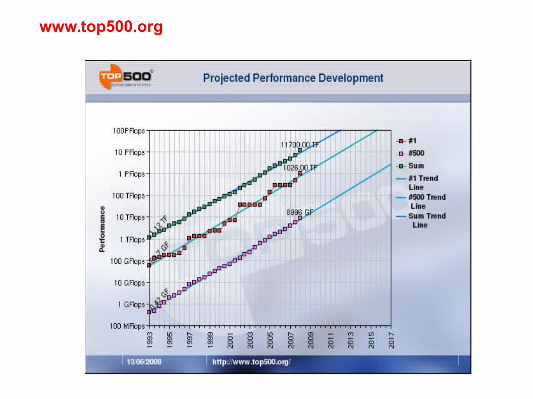
www.top500.org

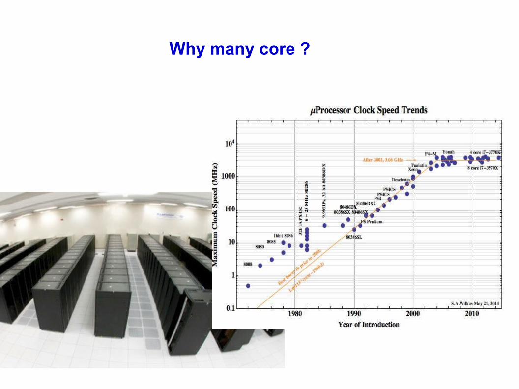
Why many core ?

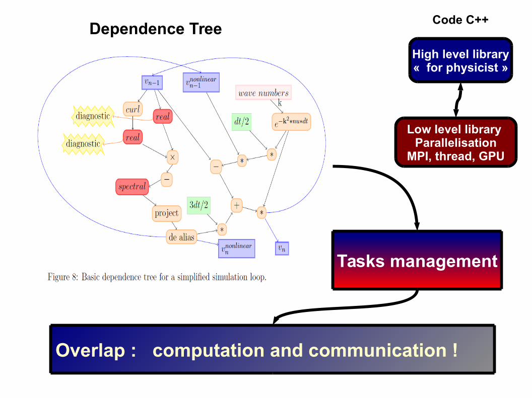
Dependence Tree

Tasks management

Overlap : computation and communication !

High level library« for physicist »

Code C++

Low level library Parallelisation

MPI, thread, GPU

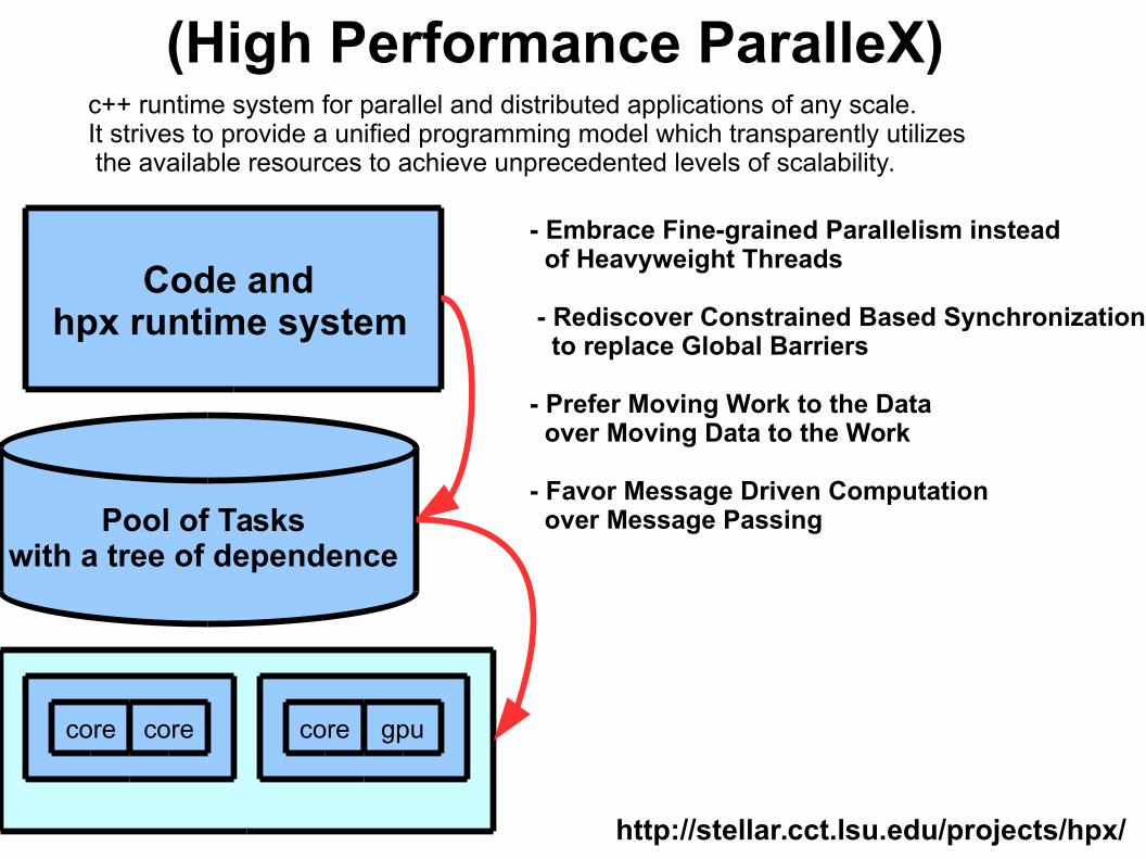
(High Performance ParalleX) c++ runtime system for parallel and distributed applications of any scale. It strives to provide a unified programming model which transparently utilizes the available resources to achieve unprecedented levels of scalability.

http://stellar.cct.lsu.edu/projects/hpx/

Code and hpx runtime system

- Embrace Fine-grained Parallelism instead of Heavyweight Threads

- Rediscover Constrained Based Synchronization to replace Global Barriers

- Prefer Moving Work to the Data over Moving Data to the Work

- Favor Message Driven Computation over Message Passing

core core core gpu

Pool of Tasks with a tree of dependence

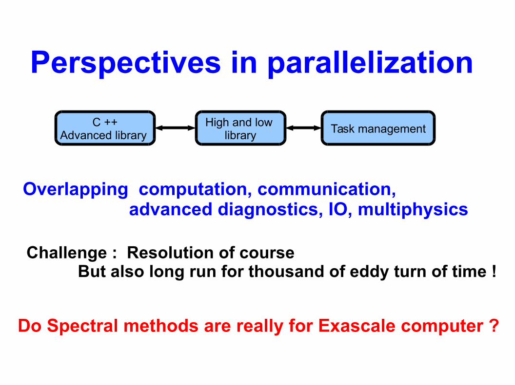
Perspectives in parallelization

C ++Advanced library

High and low library Task management

Overlapping computation, communication, advanced diagnostics, IO, multiphysics

Challenge : Resolution of course But also long run for thousand of eddy turn of time !

Do Spectral methods are really for Exascale computer ?

Diagnostics in the

?

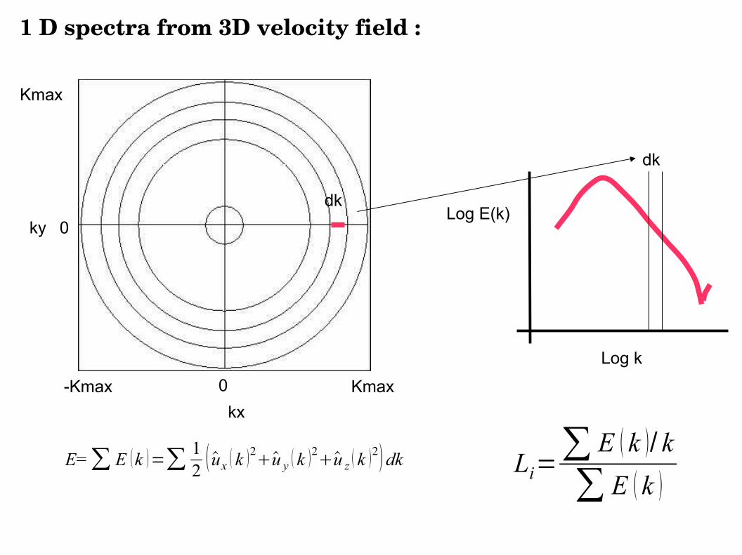
1 D spectra from 3D velocity field : 

0 Kmax-Kmax

0ky

kx

Kmax

E=∑ E k =∑12

ux k 2u y k 2u z k 2 dk

Log k

Log E(k)

dk

dk

Li=∑ E k / k

∑ E k

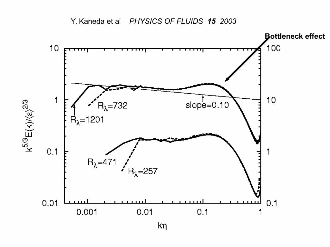
Y. Kaneda et al PHYSICS OF FLUIDS 15 2003

Bottleneck effect

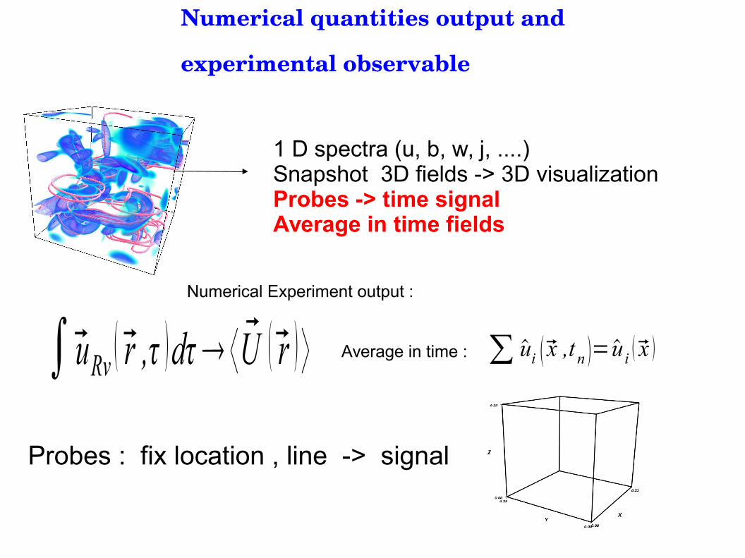
Numerical quantities output and 

experimental observable

1 D spectra (u, b, w, j, ....) Snapshot 3D fields -> 3D visualization Probes -> time signal Average in time fields

∫uRv r ,τ dτ⟨ U r ⟩ Average in time : ∑ ui x ,tn =u i x

Probes : fix location , line -> signal

Numerical Experiment output :

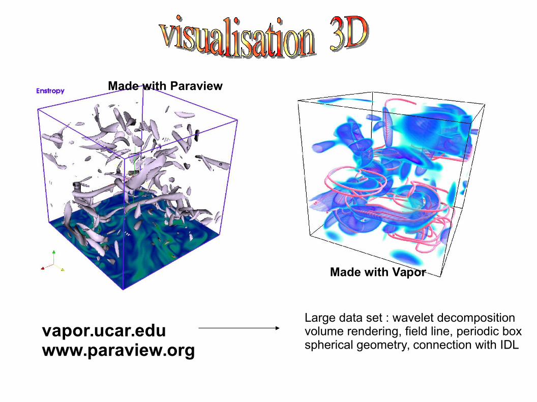
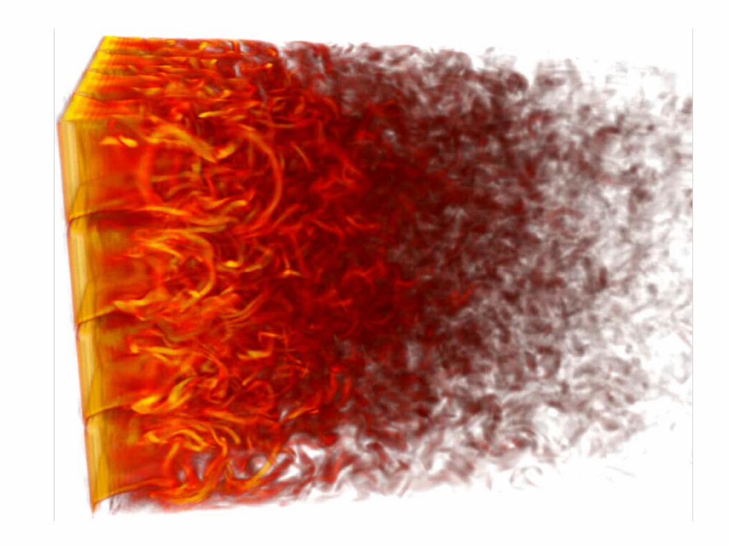
vapor.ucar.eduwww.paraview.org

Large data set : wavelet decompositionvolume rendering, field line, periodic boxspherical geometry, connection with IDL

Made with Paraview

Made with Vapor

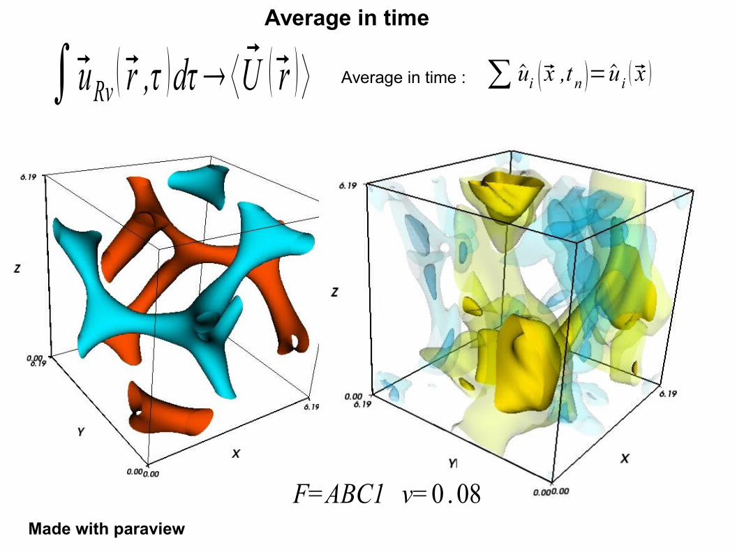
∫uRv r ,τ dτ⟨ U r ⟩ Average in time : ∑ ui x ,tn =u i x

Made with paraview

F=ABC1 ν=0 . 08

Average in time

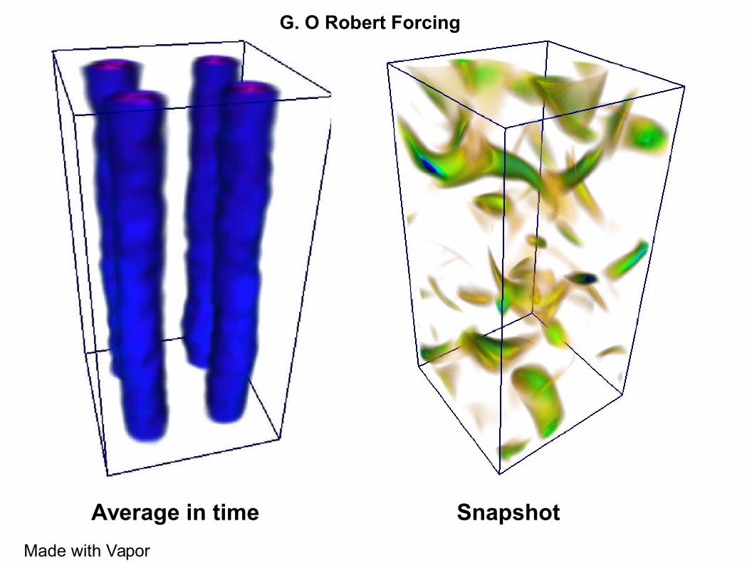
G. O Robert Forcing

Average in time Snapshot

Made with Vapor

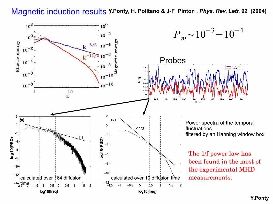
Magnetic induction results :Y.Ponty, H. Politano & J-F Pinton , Phys. Rev. Lett. 92 (2004)

Probes

Power spectra of the temporal fluctuationsfiltered by an Hanning window box

calculated over 10 diffusion timecalculated over 164 diffusion time

The 1/f power law has been found in the most of the experimental MHD measurements.

Y.Ponty

Pm ~ 10−3−10−4

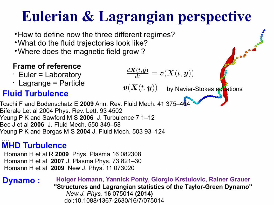
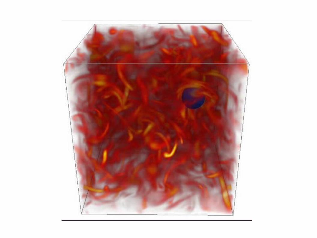
Eulerian & Lagrangian perspective

Frame of reference• Euler = Laboratory• Lagrange = Particle

How to define now the three different regimes?What do the fluid trajectories look like?Where does the magnetic field grow ?

by Navier-Stokes equations

Toschi F and Bodenschatz E 2009 Ann. Rev. Fluid Mech. 41 375–404Biferale Let al 2004 Phys. Rev. Lett. 93 4502Yeung P K and Sawford M S 2006 J. Turbulence 7 1–12Bec J et al 2006 J. Fluid Mech. 550 349–58Yeung P K and Borgas M S 2004 J. Fluid Mech. 503 93–124 ….

Fluid Turbulence

MHD Turbulence

Homann H et al R 2009 Phys. Plasma 16 082308Homann H et al 2007 J. Plasma Phys. 73 821–30Homann H et al 2009 New J. Phys. 11 073020

Holger Homann, Yannick Ponty, Giorgio Krstulovic, Rainer Grauer "Structures and Lagrangian statistics of the Taylor-Green Dynamo" New J. Phys. 16 075014 (2014) doi:10.1088/1367-2630/16/7/075014

Dynamo :

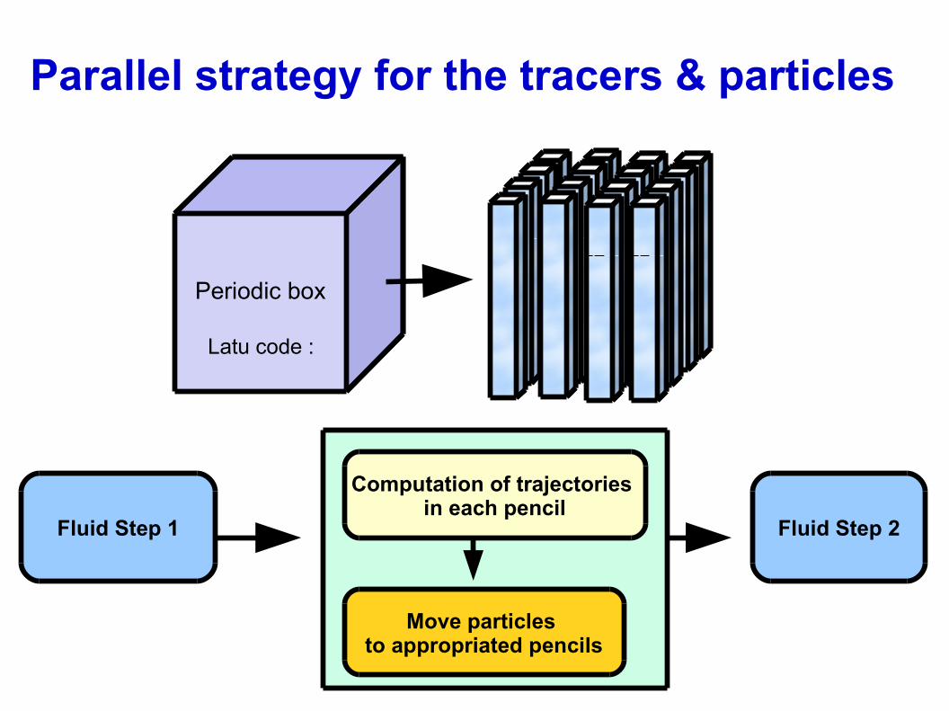
Periodic box

Latu code :

Parallel strategy for the tracers & particles

Fluid Step 1 Fluid Step 2

Computation of trajectories in each pencil

Move particles to appropriated pencils

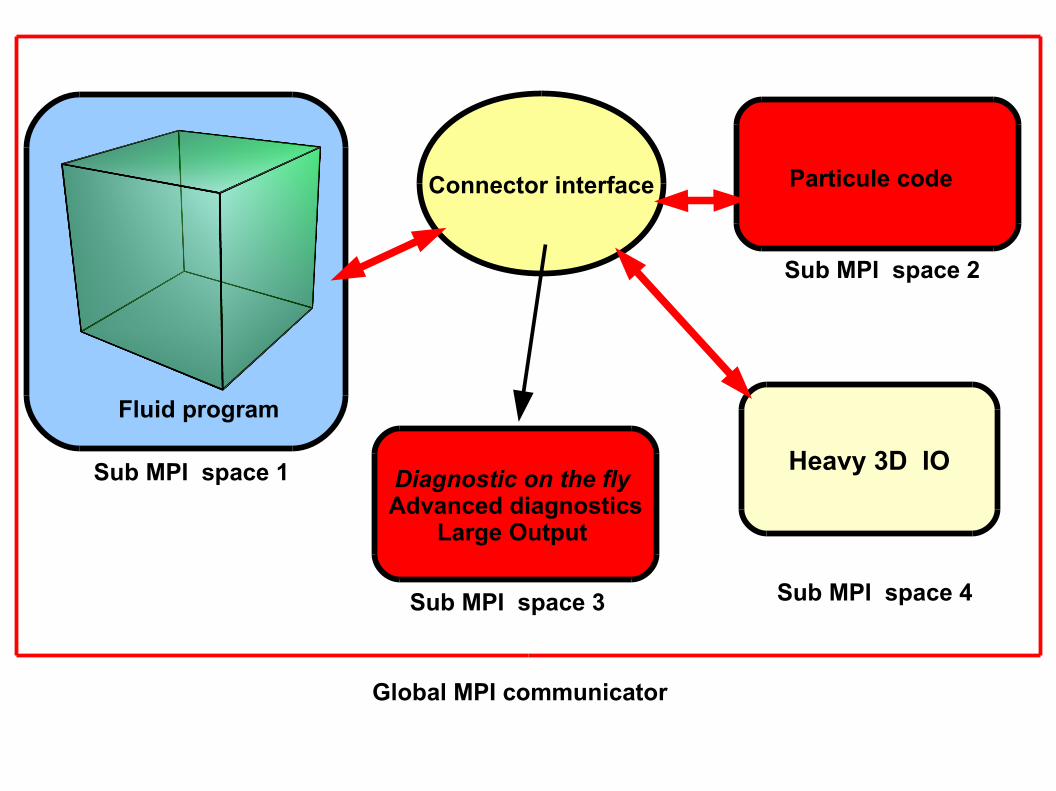
Heavy 3D IO

Fluid program

Connector interface Particule code

Diagnostic on the fly Advanced diagnostics

Large Output

Sub MPI space 1

Global MPI communicator

Sub MPI space 2

Sub MPI space 3 Sub MPI space 4

Are we able to escape from the

?

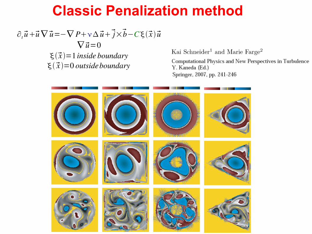
Classic Penalization method

∂t uu ∇ u=−∇ P uj×b−Cx u∇ u=0

x =1 inside boundaryx =0 outsideboundary

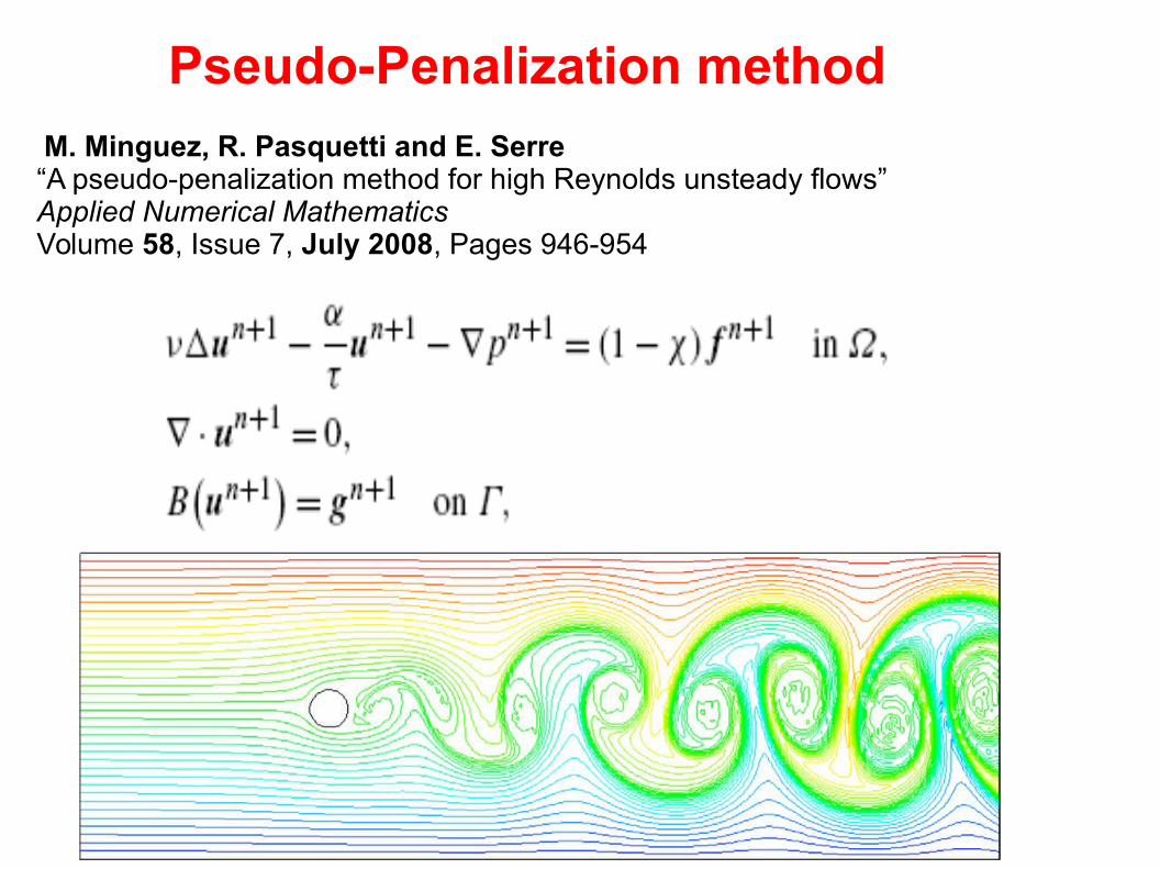
M. Minguez, R. Pasquetti and E. Serre “A pseudo-penalization method for high Reynolds unsteady flows”Applied Numerical MathematicsVolume 58, Issue 7, July 2008, Pages 946-954

Pseudo-Penalization method

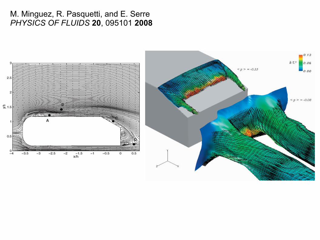
M. Minguez, R. Pasquetti, and E. SerrePHYSICS OF FLUIDS 20, 095101 2008

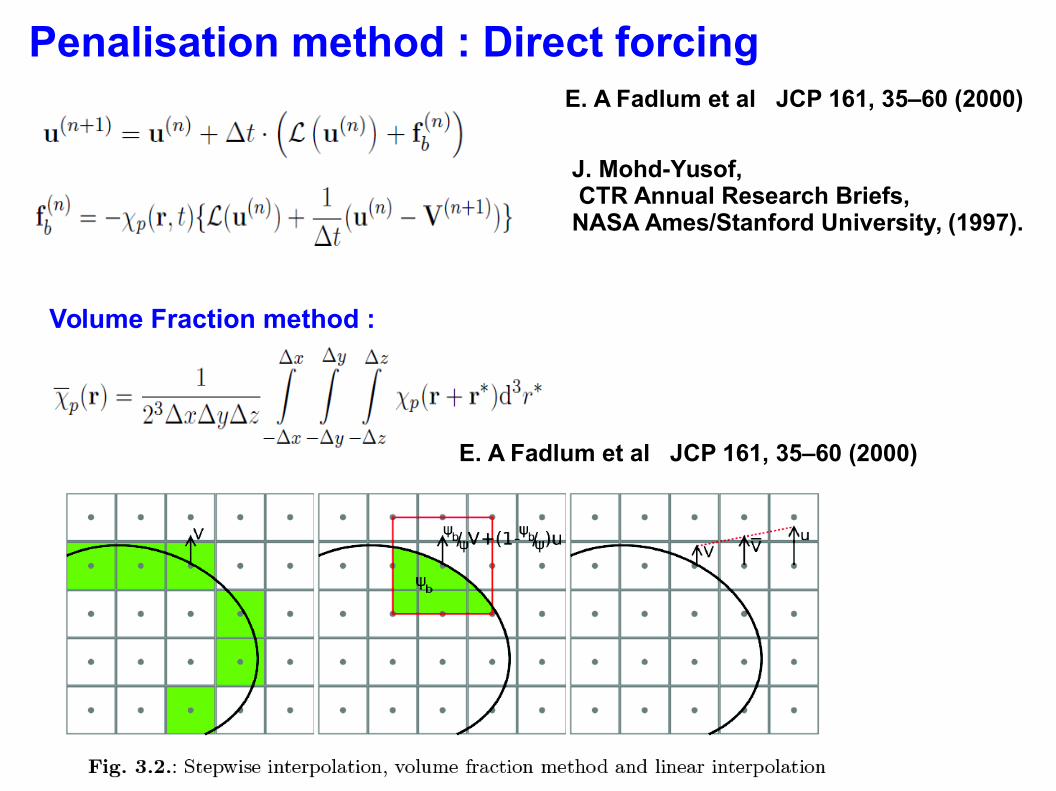
Penalisation method : Direct forcing E. A Fadlum et al JCP 161, 35–60 (2000)

Volume Fraction method :

J. Mohd-Yusof, CTR Annual Research Briefs, NASA Ames/Stanford University, (1997).

E. A Fadlum et al JCP 161, 35–60 (2000)

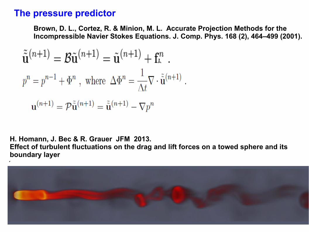
The pressure predictor

Brown, D. L., Cortez, R. & Minion, M. L. Accurate Projection Methods for theIncompressible Navier Stokes Equations. J. Comp. Phys. 168 (2), 464–499 (2001).

H. Homann, J. Bec & R. Grauer JFM 2013. Effect of turbulent fluctuations on the drag and lift forces on a towed sphere and its boundary layer

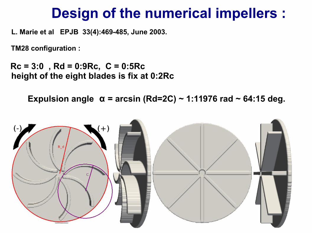
Design of the numerical impellers : L. Marie et al EPJB 33(4):469-485, June 2003.

TM28 configuration :

Rc = 3:0 , Rd = 0:9Rc, C = 0:5Rc height of the eight blades is fix at 0:2Rc

Expulsion angle α = arcsin (Rd=2C) ~ 1:11976 rad ~ 64:15 deg.

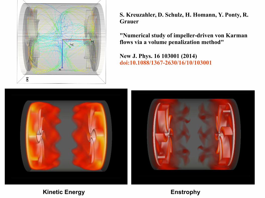
Kinetic Energy Enstrophy

S. Kreuzahler, D. Schulz, H. Homann, Y. Ponty, R. Grauer

"Numerical study of impeller-driven von Karman flows via a volume penalization method"

New J. Phys. 16 103001 (2014) doi:10.1088/1367-2630/16/10/103001

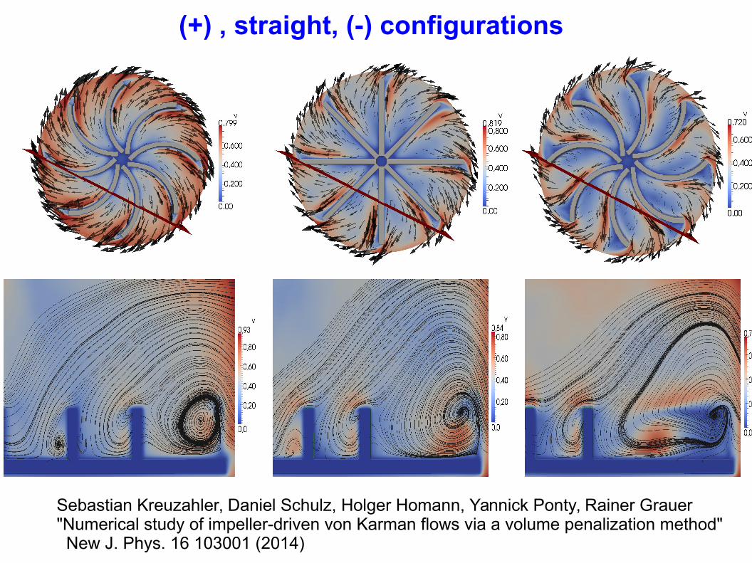
(+) , straight, (-) configurations

Sebastian Kreuzahler, Daniel Schulz, Holger Homann, Yannick Ponty, Rainer Grauer "Numerical study of impeller-driven von Karman flows via a volume penalization method" New J. Phys. 16 103001 (2014)

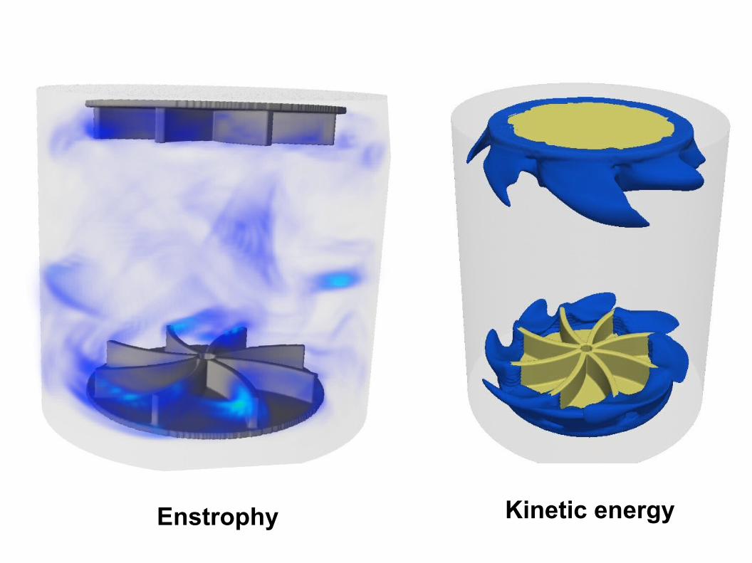
Enstrophy Kinetic energy

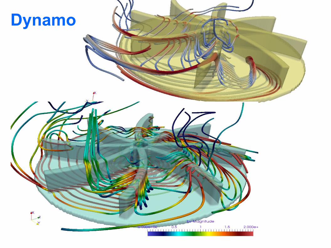
Dynamo

Pseudo­Penalization method  

Near the boundaries the schemes is accurate only order h ­> no spectral accuracy near the boundaries 

Easy to implement , versatile ­> EASY boundaries 

Prospective numerical tool

Lost of grid point  

What do you need to built a nice

?

Editor → emacs, debugger (db)Language → c++ , F90Clusters → ask to your boss or institutes

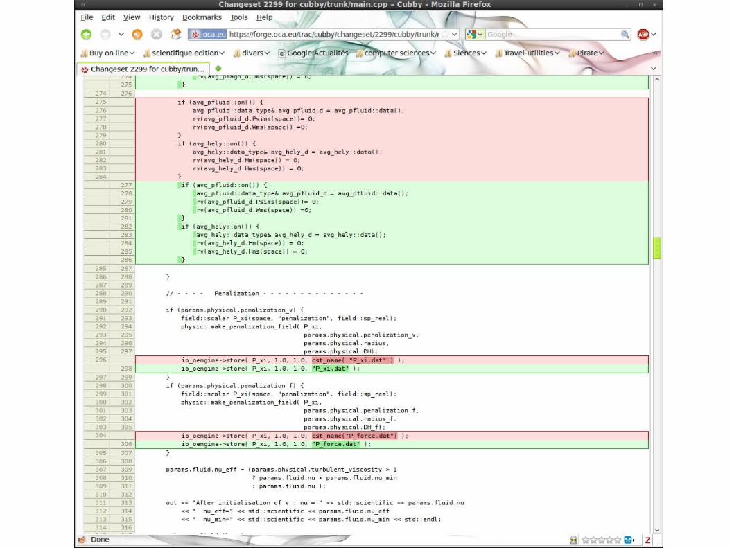
- Version saver → subversion- Wiki, ticket bug → trac

Postraitement : 3D Visualisation → paraview, vapor1D, 2D plots :

Matlab → ask to your boss

Python : matplotlib , scipy, ….

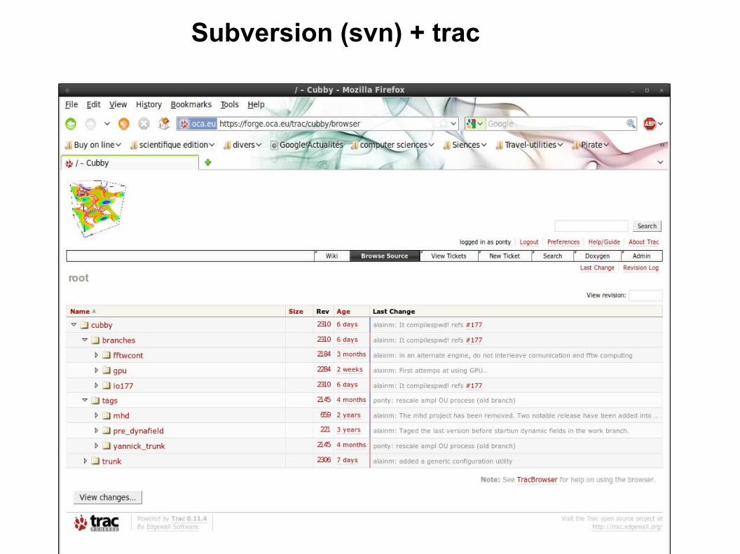
Subversion (svn) + trac

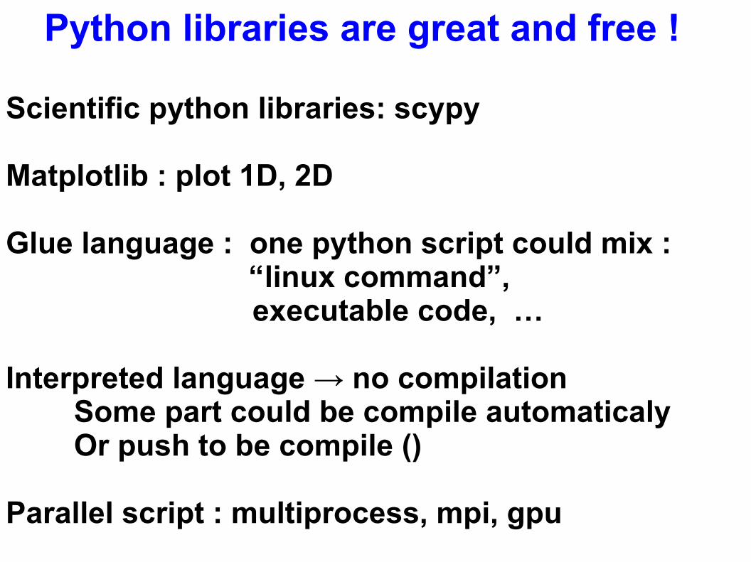
Python libraries are great and free !

Scientific python libraries: scypy

Matplotlib : plot 1D, 2D

Glue language : one python script could mix : “linux command”,

executable code, …

Interpreted language → no compilation Some part could be compile automaticaly

Or push to be compile ()

Parallel script : multiprocess, mpi, gpu

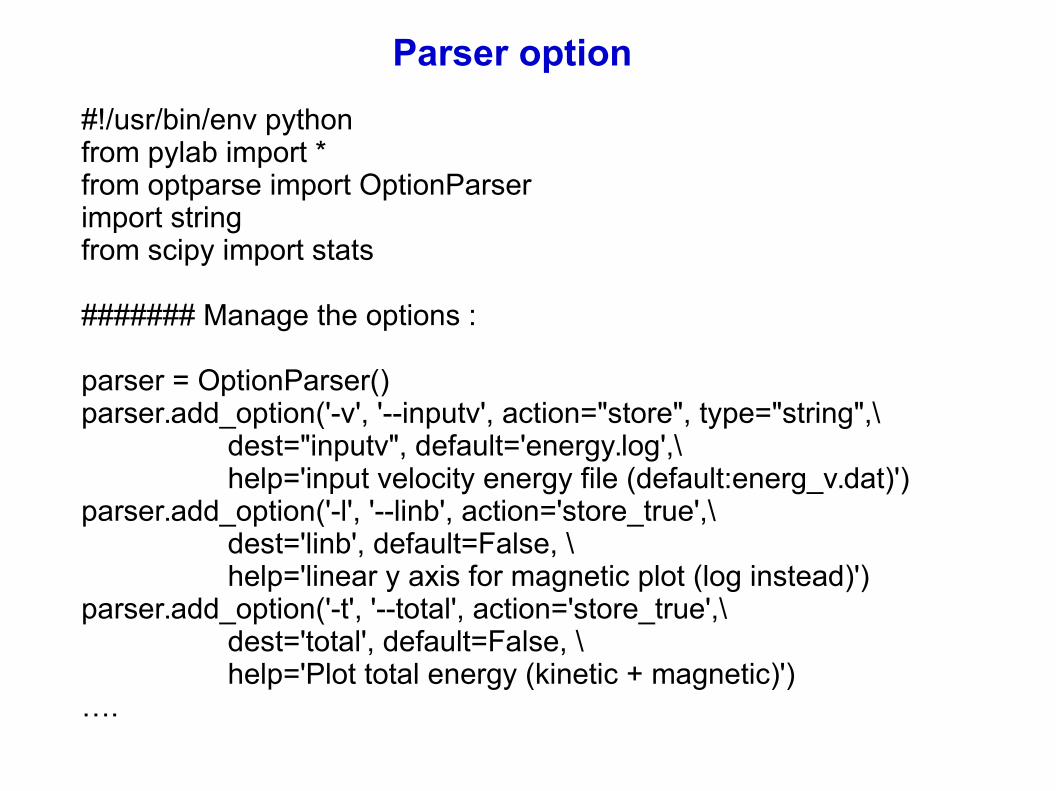
#!/usr/bin/env pythonfrom pylab import *from optparse import OptionParserimport stringfrom scipy import stats

####### Manage the options :

parser = OptionParser()parser.add_option('-v', '--inputv', action="store", type="string",\ dest="inputv", default='energy.log',\ help='input velocity energy file (default:energ_v.dat)')parser.add_option('-l', '--linb', action='store_true',\ dest='linb', default=False, \ help='linear y axis for magnetic plot (log instead)')parser.add_option('-t', '--total', action='store_true',\ dest='total', default=False, \ help='Plot total energy (kinetic + magnetic)')….

Parser option

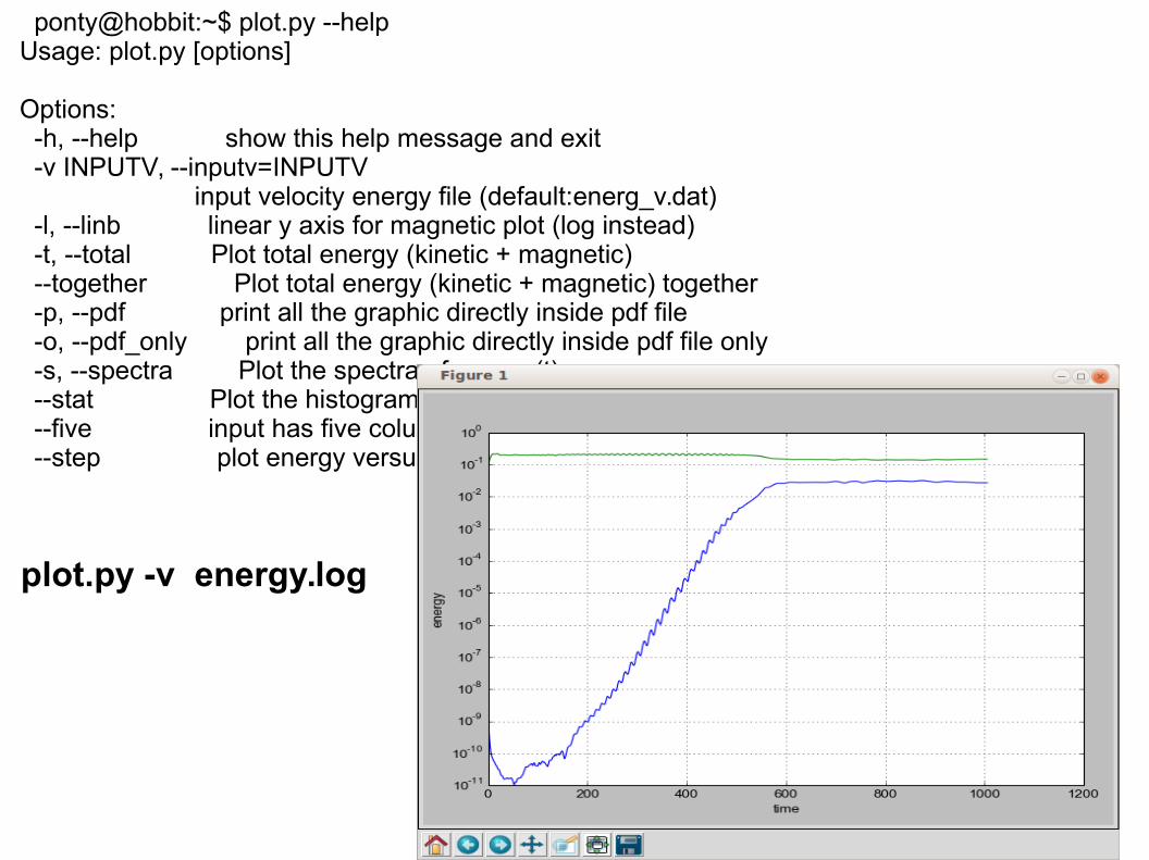
ponty@hobbit:~$ plot.py --helpUsage: plot.py [options]

Options: -h, --help show this help message and exit -v INPUTV, --inputv=INPUTV input velocity energy file (default:energ_v.dat) -l, --linb linear y axis for magnetic plot (log instead) -t, --total Plot total energy (kinetic + magnetic) --together Plot total energy (kinetic + magnetic) together -p, --pdf print all the graphic directly inside pdf file -o, --pdf_only print all the graphic directly inside pdf file only -s, --spectra Plot the spectra of energy(t) --stat Plot the histogram of energy(t) and give stat values --five input has five columm instead of six --step plot energy versus step

plot.py -v energy.log

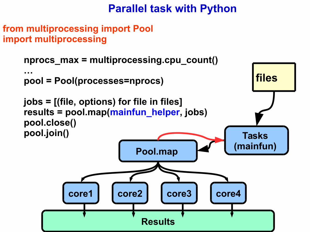
from multiprocessing import Poolimport multiprocessing nprocs_max = multiprocessing.cpu_count() … pool = Pool(processes=nprocs)

jobs = [(file, options) for file in files] results = pool.map(mainfun_helper, jobs) pool.close() pool.join()

Parallel task with Python

files

Tasks (mainfun)

core1 core2 core3 core4

Pool.map

Results

Impossible to escapeThen Join the 

?

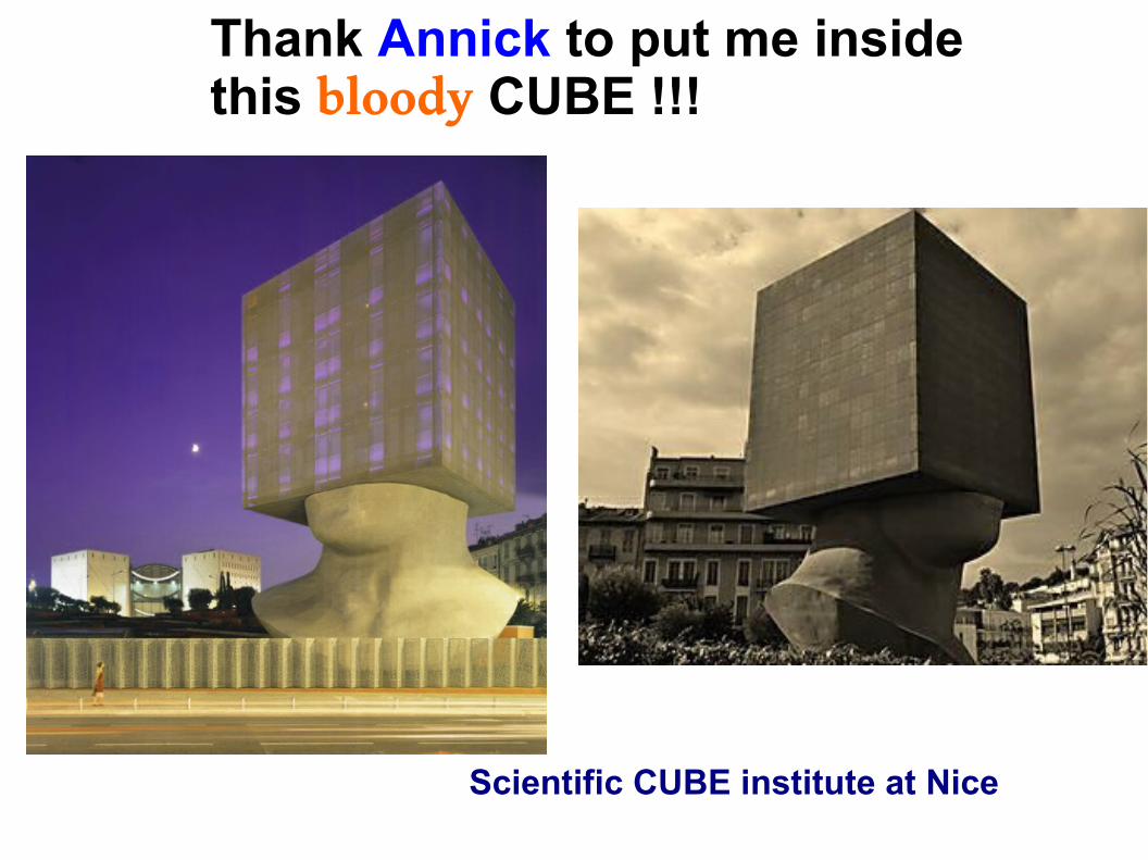
Scientific CUBE institute at Nice

Thank Annick to put me inside this bloody CUBE !!!