On Nonlinear Dispersive Equations in Periodic Structures ... · Structures: Semiclassical Limits...
52
On Nonlinear Dispersive Equations in Periodic Structures: Semiclassical Limits and Numerical Methods Peter A. Markowich Department of Applied Mathematics and Theoretical Physics, University of Cambridge June 6, 2008 P. A. Markowich (DAMTP,U. of Cambridge) Nonlinear Dispersive Equations June 6, 2008 1 / 38
Transcript of On Nonlinear Dispersive Equations in Periodic Structures ... · Structures: Semiclassical Limits...
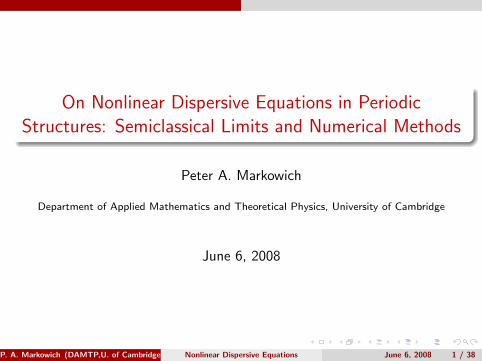
On Nonlinear Dispersive Equations in PeriodicStructures: Semiclassical Limits and Numerical Methods
Peter A. Markowich
Department of Applied Mathematics and Theoretical Physics, University of Cambridge
June 6, 2008
P. A. Markowich (DAMTP,U. of Cambridge) Nonlinear Dispersive Equations June 6, 2008 1 / 38
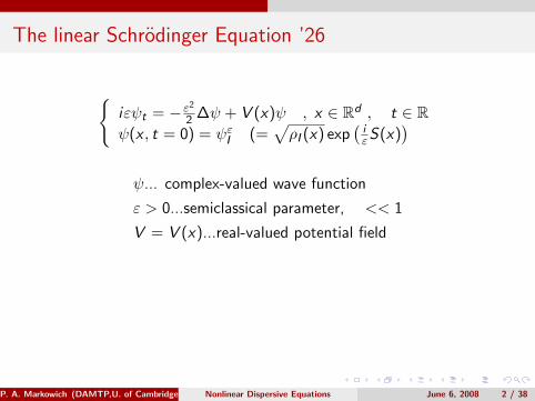
The linear Schrodinger Equation ’26
{iεψt = − ε2
2 ∆ψ + V (x)ψ , x ∈ Rd , t ∈ Rψ(x , t = 0) = ψεI (=
√ρI (x) exp
(iεS(x)
)ψ... complex-valued wave function
ε > 0...semiclassical parameter, << 1
V = V (x)...real-valued potential field
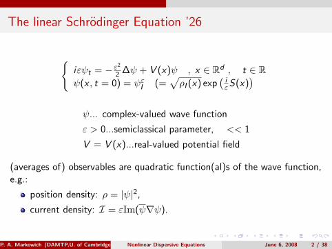
(averages of) observables are quadratic function(al)s of the wave function,e.g.:
position density: ρ = |ψ|2,
current density: I = εIm(ψ∇ψ).
P. A. Markowich (DAMTP,U. of Cambridge) Nonlinear Dispersive Equations June 6, 2008 2 / 38
The linear Schrodinger Equation ’26
{iεψt = − ε2
2 ∆ψ + V (x)ψ , x ∈ Rd , t ∈ Rψ(x , t = 0) = ψεI (=
√ρI (x) exp
(iεS(x)
)ψ... complex-valued wave function
ε > 0...semiclassical parameter, << 1
V = V (x)...real-valued potential field
(averages of) observables are quadratic function(al)s of the wave function,e.g.:
position density: ρ = |ψ|2,
current density: I = εIm(ψ∇ψ).
P. A. Markowich (DAMTP,U. of Cambridge) Nonlinear Dispersive Equations June 6, 2008 2 / 38
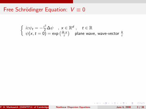
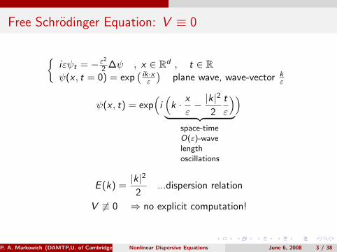
Free Schrodinger Equation: V ≡ 0
{iεψt = − ε2
2 ∆ψ , x ∈ Rd , t ∈ Rψ(x , t = 0) = exp
(ik·xε
)plane wave, wave-vector k
ε
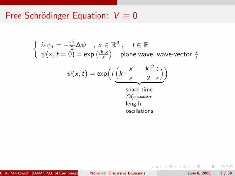
ψ(x , t) = exp(
i(
k · x
ε− |k |
2
2
t
ε
)︸ ︷︷ ︸
space-timeO(ε)-wavelengthoscillations
)
E (k) =|k |2
2...dispersion relation
V 6≡ 0 ⇒ no explicit computation!
P. A. Markowich (DAMTP,U. of Cambridge) Nonlinear Dispersive Equations June 6, 2008 3 / 38
Free Schrodinger Equation: V ≡ 0
{iεψt = − ε2
2 ∆ψ , x ∈ Rd , t ∈ Rψ(x , t = 0) = exp
(ik·xε
)plane wave, wave-vector k
ε
ψ(x , t) = exp(
i(
k · x
ε− |k |
2
2
t
ε
)︸ ︷︷ ︸
space-timeO(ε)-wavelengthoscillations
)
E (k) =|k |2
2...dispersion relation
V 6≡ 0 ⇒ no explicit computation!
P. A. Markowich (DAMTP,U. of Cambridge) Nonlinear Dispersive Equations June 6, 2008 3 / 38
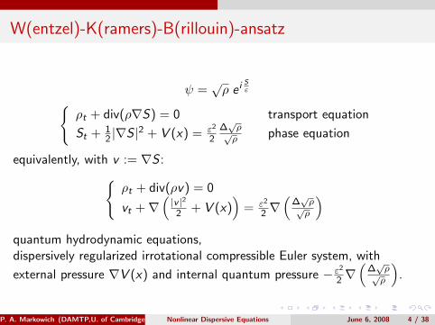
W(entzel)-K(ramers)-B(rillouin)-ansatz
ψ =√ρ e i S
ε{ρt + div(ρ∇S) = 0 transport equation
St + 12 |∇S |2 + V (x) = ε2
2∆√ρ√ρ phase equation
equivalently, with v := ∇S :{ρt + div(ρv) = 0
vt +∇(|v |2
2 + V (x))
= ε2
2 ∇(
∆√ρ√ρ
)quantum hydrodynamic equations,dispersively regularized irrotational compressible Euler system, with
external pressure ∇V (x) and internal quantum pressure − ε2
2 ∇(
∆√ρ√ρ
).
P. A. Markowich (DAMTP,U. of Cambridge) Nonlinear Dispersive Equations June 6, 2008 4 / 38
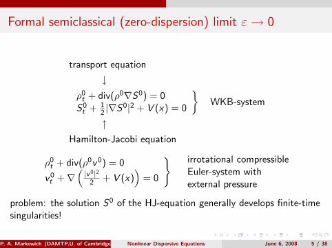
Formal semiclassical (zero-dispersion) limit ε→ 0
transport equation
↓ρ0t + div(ρ0∇S0) = 0
S0t + 1
2 |∇S0|2 + V (x) = 0
}WKB-system
↑Hamilton-Jacobi equation
ρ0t + div(ρ0v 0) = 0
v 0t +∇
(|v0|2
2 + V (x))
= 0
} irrotational compressibleEuler-system withexternal pressure
problem: the solution S0 of the HJ-equation generally develops finite-timesingularities!
P. A. Markowich (DAMTP,U. of Cambridge) Nonlinear Dispersive Equations June 6, 2008 5 / 38
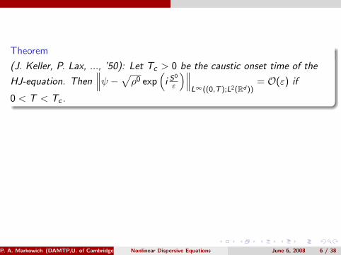
Theorem
(J. Keller, P. Lax, ..., ’50): Let Tc > 0 be the caustic onset time of the
HJ-equation. Then∥∥∥ψ −√ρ0 exp
(i S0
ε
)∥∥∥L∞((0,T );L2(Rd ))
= O(ε) if
0 < T < Tc .
beyond caustics:
V. Maslov ’60: phase shifts
P. Gerard, P. Markowich, N. Mauser, F. Poupaud, P.L. Lions, T. Paul,C. Sparber ’90-’08: semiclassical (Wigner) measures
S. Jin, S. Osher ’02-’08; C. Sparber, P. Markowich, N. Mauser ’01:multi-valued solutions of HJ-equations
P. A. Markowich (DAMTP,U. of Cambridge) Nonlinear Dispersive Equations June 6, 2008 6 / 38
Semiclassical (Wigner) Measures
Definition
Let ψε ∈ L2(Rd) be a sequence of wave functions and (ε)→ 0 a scale.Then w ∈M+(Rd
x × Rdξ ) is called a semiclassical measure of ψε on the
scale (ε) if for all a ∈ S(Rdx × Rd
ξ ), along a subsequence:
limε→0
∫Rd
ψε(x)aw (x , εD)ψε dx =
∫Rd
x×Rdξ
a(x , ξ)w(dx , dξ).
Theorem
(’80 folklore) The semiclassical measure(s) w = w(x , ξ, t) of the solutionψε(t) of the IVP-problem for the Schrodinger equation satisfies(y) theLiouville equation{
wt + ξ · ∇xw −∇xV · ∇ξw = 0 on Rdx × Rd
ξ × Rt
w(t = 0) = wI (a semiclassical measure of ψεI ).
P. A. Markowich (DAMTP,U. of Cambridge) Nonlinear Dispersive Equations June 6, 2008 7 / 38
Connection to WKB-Asymptotics:
If ψI (x) =√ρI (x) exp
(SI (x)ε
), then wI (x , ξ) = ρI (x)δ(ξ −∇SI (x)).
The solution of the Liouville equation stays monokinetic
w(x , ξ, t) = ρ0(x , t)δ(ξ −∇S0(x , t))
as long as S0 is the smooth solution of the HJ-equation{S0
t + 12 |∇S0|2 + V (x) = 0
S0(x , t = 0) = SI (x) .
After caustic onset: multi-valued solution theory (C. Sparber, P.Markowich, N. Mauser ’02; S. Jin, S. Osher ’04)!
P. A. Markowich (DAMTP,U. of Cambridge) Nonlinear Dispersive Equations June 6, 2008 8 / 38
Nonlinear Schrodinger Equations: V = f (ρ)
{iεψt = − ε2
2 ∆ψ + f (|ψ|2)ψ , x ∈ Rd , t > 0 ,
ψ(t = 0) =√ρI exp
(i SIε
), ρI , SI smooth
formal (compressible, isentropic, irrotational) Euler limit as ε→ 0:{ρ0t + div(ρ0v 0) = 0 , ρ0(t = 0) = ρI ,
v 0t +∇
(12 |v
0|2 + f (ρ0))
= 0 , v 0(t = 0) = ∇SI
Theorem
(E. Grenier ’98; R. Carles ’07): f ′ > 0 on R+. Let T > 0 be smaller than the maximalexistence time (of smooth solutions) of the irrotational isentropic Euler system. Then‚‚‚‚ψ −pρ0 exp
„iS0
ε
«‚‚‚‚L∞((0,T );Hs (Rd ))
ε→0−→ 0 for some s > 0 .
Proof: Theory of symmetric hyperbolic systems, energy estimates.
P. A. Markowich (DAMTP,U. of Cambridge) Nonlinear Dispersive Equations June 6, 2008 9 / 38
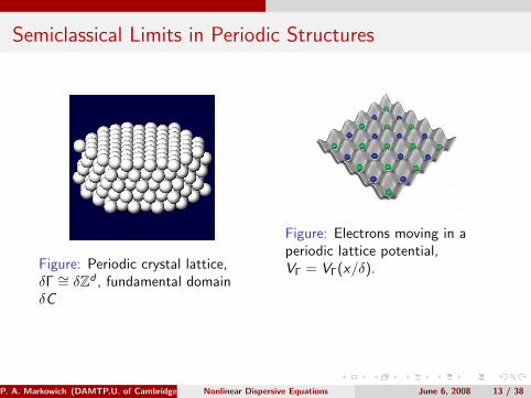
Semiclassical Limits in Periodic Structures
Figure: Periodic crystal lattice,δΓ ∼= δZd , fundamental domainδC
Figure: Electrons moving in aperiodic lattice potential,VΓ = VΓ(x/δ).
Assumption: lattice spacing δ=semiclassical parameter ε
NLS: iεψt = −ε2
2∆ψ + VΓ
(x
ε
)ψ + V (x)ψ︸ ︷︷ ︸
slow-fast coupling
+ κ(ε)|ψ|2ψ︸ ︷︷ ︸binary interaction
P. A. Markowich (DAMTP,U. of Cambridge) Nonlinear Dispersive Equations June 6, 2008 13 / 38
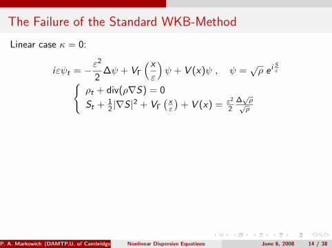
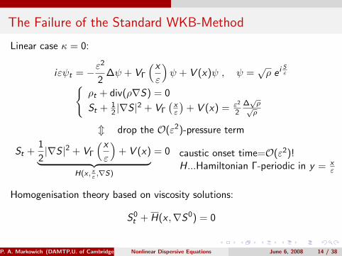
The Failure of the Standard WKB-Method
Linear case κ = 0:
iεψt = −ε2
2∆ψ + VΓ
(x
ε
)ψ + V (x)ψ , ψ =
√ρ e i S
ε{ρt + div(ρ∇S) = 0
St + 12 |∇S |2 + VΓ
(xε
)+ V (x) = ε2
2∆√ρ√ρ
m drop the O(ε2)-pressure term
St +1
2|∇S |2 + VΓ
(x
ε
)+ V (x)︸ ︷︷ ︸
H(x , xε,∇S)
= 0 caustic onset time=O(ε2)!H...Hamiltonian Γ-periodic in y = x
ε
Homogenisation theory based on viscosity solutions:
S0t + H(x ,∇S0) = 0
P. A. Markowich (DAMTP,U. of Cambridge) Nonlinear Dispersive Equations June 6, 2008 14 / 38
Effective Hamiltonian H = H(x , ξ): obtained by solving a stationaryHJ-equation on a lattice cell.
References: P.L. Lions, G. Papanicolaou, S. Varadhan ’96; D. Gomes,L. Evans, P. Souganidis, P.L Lions ’02-’08.
Problem: viscosity solutions are based on a notion of dissipativity ⇒loss of reversibility! But: the Schrodinger equation is time reversible!
P. A. Markowich (DAMTP,U. of Cambridge) Nonlinear Dispersive Equations June 6, 2008 15 / 38
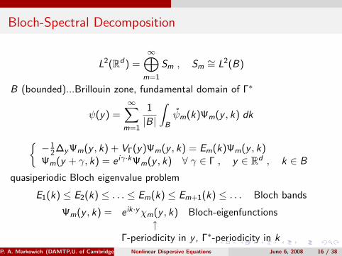
Bloch-Spectral Decomposition
L2(Rd) =∞⊕
m=1
Sm , Sm∼= L2(B)
B (bounded)...Brillouin zone, fundamental domain of Γ∗
ψ(y) =∞∑
m=1
1
|B|
∫Bψm(k)Ψm(y , k) dk
{−1
2 ∆y Ψm(y , k) + VΓ(y)Ψm(y , k) = Em(k)Ψm(y , k)Ψm(y + γ, k) = e iγ·kΨm(y , k) ∀ γ ∈ Γ , y ∈ Rd , k ∈ B
quasiperiodic Bloch eigenvalue problem
E1(k) ≤ E2(k) ≤ . . . ≤ Em(k) ≤ Em+1(k) ≤ . . . Bloch bands
Ψm(y , k) = e ik·yχm(y , k) Bloch-eigenfunctions↑
Γ-periodicity in y , Γ∗-periodicity in kP. A. Markowich (DAMTP,U. of Cambridge) Nonlinear Dispersive Equations June 6, 2008 16 / 38
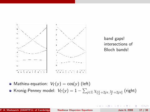
band gaps!intersections ofBloch bands!
Mathieu-equation: VΓ(y) = cos(y) (left)
Kronig-Penney model: VΓ(y) = 1−∑
j∈Z χ[π2
+2jπ, 3π2
+2jπ] (right)
P. A. Markowich (DAMTP,U. of Cambridge) Nonlinear Dispersive Equations June 6, 2008 17 / 38
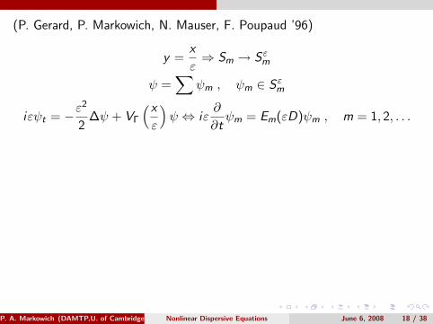
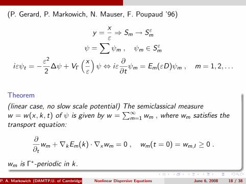
(P. Gerard, P. Markowich, N. Mauser, F. Poupaud ’96)
y =x
ε⇒ Sm → Sεm
ψ =∑
ψm , ψm ∈ Sεm
iεψt = −ε2
2∆ψ + VΓ
(x
ε
)ψ ⇔ iε
∂
∂tψm = Em(εD)ψm , m = 1, 2, . . .
Theorem
(linear case, no slow scale potential) The semiclassical measurew = w(x , k , t) of ψ is given by w =
∑∞m=1 wm , where wm satisfies the
transport equation:
∂
∂twm +∇kEm(k) · ∇xwm = 0 , wm(t = 0) = wm,I ≥ 0 .
wm is Γ∗-periodic in k.
P. A. Markowich (DAMTP,U. of Cambridge) Nonlinear Dispersive Equations June 6, 2008 18 / 38
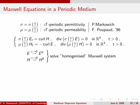
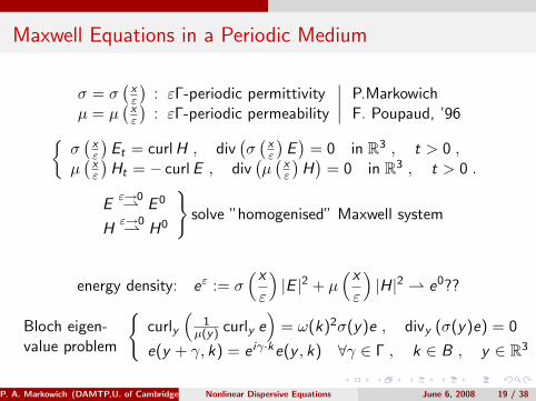
Maxwell Equations in a Periodic Medium
σ = σ(
xε
): εΓ-periodic permittivity
µ = µ(
xε
): εΓ-periodic permeability
∣∣∣∣ P.MarkowichF. Poupaud, ’96{
σ(
xε
)Et = curl H , div
(σ(
xε
)E)
= 0 in R3 , t > 0 ,µ(
xε
)Ht = − curl E , div
(µ(
xε
)H)
= 0 in R3 , t > 0 .
Eε→0⇀ E 0
Hε→0⇀ H0
}solve ”homogenised” Maxwell system
energy density: eε := σ(x
ε
)|E |2 + µ
(x
ε
)|H|2 ⇀ e0??
Bloch eigen-value problem
{curly
(1
µ(y) curly e)
= ω(k)2σ(y)e , divy (σ(y)e) = 0
e(y + γ, k) = e iγ·ke(y , k) ∀γ ∈ Γ , k ∈ B , y ∈ R3
P. A. Markowich (DAMTP,U. of Cambridge) Nonlinear Dispersive Equations June 6, 2008 19 / 38
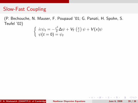
Slow-Fast Coupling
(P. Bechouche, N. Mauser, F. Poupaud ’01; G. Panati, H. Spohn, S.Teufel ’02) {
iεψt = − ε2
2 ∆ψ + VΓ
(xε
)ψ + V (x)ψ
ψ(t = 0) = ψI
Theorem
Let ψI concentrate in the m-th Bloch band space Sεm and assume that them-th band Em = Em(k) is isolated. Then the semiclassical measure ofψ(t) satisfies{
wt +∇kEm(k) · ∇xw −∇xV (x) · ∇kw = 0w(t = 0) = wI (= a semiclassical measure of ψI ).
If wI = ρI (x)δΓ∗(k −∇SI (x)), then w(t) = ρ(x , t)δΓ∗(k −∇S(x , t)) aslong as S remains smooth, where{
St + Em(∇S) + V (x) = 0S(t = 0) = SI
P. A. Markowich (DAMTP,U. of Cambridge) Nonlinear Dispersive Equations June 6, 2008 20 / 38
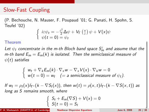
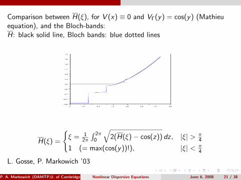
Comparison between H(ξ), for V (x) ≡ 0 and VΓ(y) = cos(y) (Mathieuequation), and the Bloch-bands:H: black solid line, Bloch bands: blue dotted lines
H(ξ) =
{ξ = 1
2π
∫ 2π0
√2(H(ξ)− cos(z)) dz , |ξ| > π
4
1 (= max(cos(y))!), |ξ| < π4
L. Gosse, P. Markowich ’03
P. A. Markowich (DAMTP,U. of Cambridge) Nonlinear Dispersive Equations June 6, 2008 21 / 38
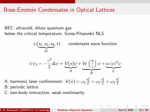
Bose-Einstein Condensates in Optical Lattices
BEC: ultracold, dilute quantum gasbelow the critical temperature: Gross-Pitaevskii NLS
ψ(x1, x2, x3︸ ︷︷ ︸R3
, t) : condensate wave function
iεψt = −ε2
2∆ψ + V (x)ψ︸ ︷︷ ︸
A
+ VΓ
(x
ε
)ψ︸ ︷︷ ︸
B
+κε|ψ|2ψ︸ ︷︷ ︸C
A: harmonic laser confinement: V (x) = ω1x2
12 + ω2
x222 + ω3
x232
B: periodic latticeC: two-body interaction, weak nonlinearity
P. A. Markowich (DAMTP,U. of Cambridge) Nonlinear Dispersive Equations June 6, 2008 22 / 38
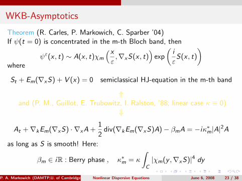
WKB-Asymptotics
Theorem (R. Carles, P. Markowich, C. Sparber ’04)If ψ(t = 0) is concentrated in the m-th Bloch band, then
ψε(x , t) ∼ A(x , t)χm
(x
ε,∇xS(x , t)
)exp
(i
εS(x , t)
)where
St + Em(∇xS) + V (x) = 0 semiclassical HJ-equation in the m-th band
⇑and (P. M., Guillot, E. Trubowitz, I. Ralston, ’88; linear case κ ≡ 0)
⇓
At +∇kEm(∇xS) · ∇xA +1
2div(∇kEm(∇xS)A)− βmA = −iκ∗m|A|2A
as long as S is smooth! Here:
βm ∈ iR : Berry phase , κ∗m = κ
∫C|χm(y ,∇xS)|4 dy
P. A. Markowich (DAMTP,U. of Cambridge) Nonlinear Dispersive Equations June 6, 2008 23 / 38
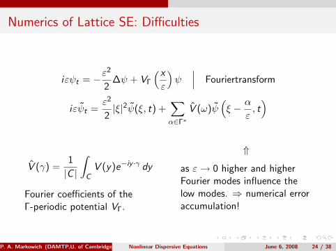
Numerics of Lattice SE: Difficulties
iεψt = −ε2
2∆ψ + VΓ
(x
ε
)ψ
∣∣∣ Fouriertransform
iεψt =ε2
2|ξ|2ψ(ξ, t) +
∑α∈Γ∗
V (ω)ψ(ξ − α
ε, t)
V (γ) =1
|C |
∫C
V (y)e−iy ·γ dy
Fourier coefficients of theΓ-periodic potential VΓ.
⇑
as ε→ 0 higher and higherFourier modes influence thelow modes. ⇒ numerical erroraccumulation!
P. A. Markowich (DAMTP,U. of Cambridge) Nonlinear Dispersive Equations June 6, 2008 24 / 38
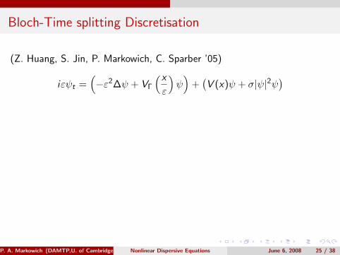
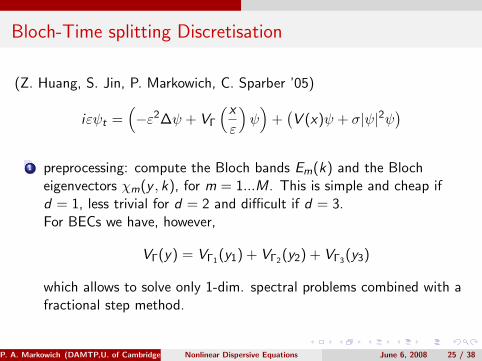
Bloch-Time splitting Discretisation
(Z. Huang, S. Jin, P. Markowich, C. Sparber ’05)
iεψt =(−ε2∆ψ + VΓ
(x
ε
)ψ)
+(V (x)ψ + σ|ψ|2ψ
)
1 preprocessing: compute the Bloch bands Em(k) and the Blocheigenvectors χm(y , k), for m = 1...M. This is simple and cheap ifd = 1, less trivial for d = 2 and difficult if d = 3.For BECs we have, however,
VΓ(y) = VΓ1(y1) + VΓ2(y2) + VΓ3(y3)
which allows to solve only 1-dim. spectral problems combined with afractional step method.
P. A. Markowich (DAMTP,U. of Cambridge) Nonlinear Dispersive Equations June 6, 2008 25 / 38
Bloch-Time splitting Discretisation
(Z. Huang, S. Jin, P. Markowich, C. Sparber ’05)
iεψt =(−ε2∆ψ + VΓ
(x
ε
)ψ)
+(V (x)ψ + σ|ψ|2ψ
)1 preprocessing: compute the Bloch bands Em(k) and the Bloch
eigenvectors χm(y , k), for m = 1...M. This is simple and cheap ifd = 1, less trivial for d = 2 and difficult if d = 3.For BECs we have, however,
VΓ(y) = VΓ1(y1) + VΓ2(y2) + VΓ3(y3)
which allows to solve only 1-dim. spectral problems combined with afractional step method.
P. A. Markowich (DAMTP,U. of Cambridge) Nonlinear Dispersive Equations June 6, 2008 25 / 38
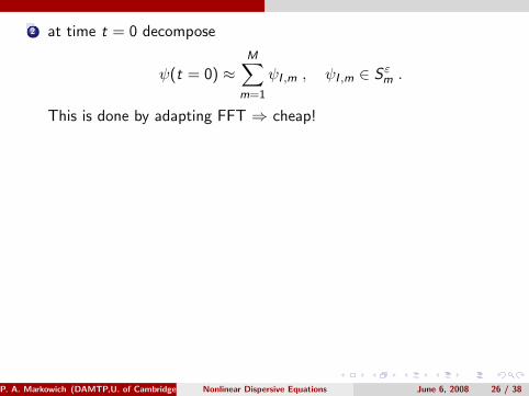
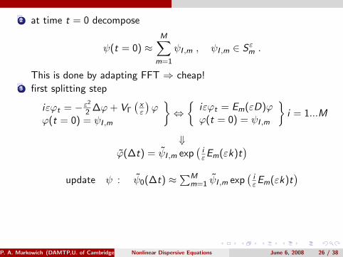
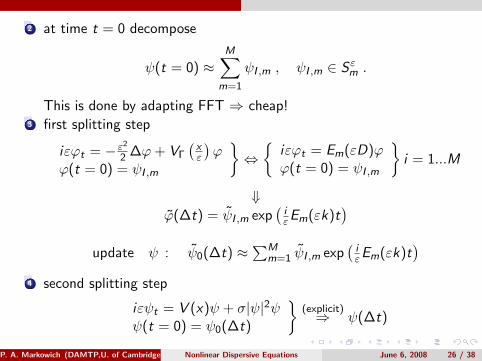
2 at time t = 0 decompose
ψ(t = 0) ≈M∑
m=1
ψI ,m , ψI ,m ∈ Sεm .
This is done by adapting FFT ⇒ cheap!
3 first splitting step
iεϕt = − ε2
2 ∆ϕ+ VΓ
(xε
)ϕ
ϕ(t = 0) = ψI ,m
}⇔{
iεϕt = Em(εD)ϕϕ(t = 0) = ψI ,m
}i = 1...M
⇓ϕ(∆t) = ψI ,m exp
(iεEm(εk)t
)update ψ : ψ0(∆t) ≈
∑Mm=1 ψI ,m exp
(iεEm(εk)t
)4 second splitting step
iεψt = V (x)ψ + σ|ψ|2ψψ(t = 0) = ψ0(∆t)
}(explicit)⇒ ψ(∆t)
P. A. Markowich (DAMTP,U. of Cambridge) Nonlinear Dispersive Equations June 6, 2008 26 / 38
2 at time t = 0 decompose
ψ(t = 0) ≈M∑
m=1
ψI ,m , ψI ,m ∈ Sεm .
This is done by adapting FFT ⇒ cheap!3 first splitting step
iεϕt = − ε2
2 ∆ϕ+ VΓ
(xε
)ϕ
ϕ(t = 0) = ψI ,m
}⇔{
iεϕt = Em(εD)ϕϕ(t = 0) = ψI ,m
}i = 1...M
⇓ϕ(∆t) = ψI ,m exp
(iεEm(εk)t
)update ψ : ψ0(∆t) ≈
∑Mm=1 ψI ,m exp
(iεEm(εk)t
)
4 second splitting step
iεψt = V (x)ψ + σ|ψ|2ψψ(t = 0) = ψ0(∆t)
}(explicit)⇒ ψ(∆t)
P. A. Markowich (DAMTP,U. of Cambridge) Nonlinear Dispersive Equations June 6, 2008 26 / 38
2 at time t = 0 decompose
ψ(t = 0) ≈M∑
m=1
ψI ,m , ψI ,m ∈ Sεm .
This is done by adapting FFT ⇒ cheap!3 first splitting step
iεϕt = − ε2
2 ∆ϕ+ VΓ
(xε
)ϕ
ϕ(t = 0) = ψI ,m
}⇔{
iεϕt = Em(εD)ϕϕ(t = 0) = ψI ,m
}i = 1...M
⇓ϕ(∆t) = ψI ,m exp
(iεEm(εk)t
)update ψ : ψ0(∆t) ≈
∑Mm=1 ψI ,m exp
(iεEm(εk)t
)4 second splitting step
iεψt = V (x)ψ + σ|ψ|2ψψ(t = 0) = ψ0(∆t)
}(explicit)⇒ ψ(∆t)
P. A. Markowich (DAMTP,U. of Cambridge) Nonlinear Dispersive Equations June 6, 2008 26 / 38
Remarks on the Bloch-time splitting scheme
1 a second order Strang-splitting scheme is straightforward
2 meshsize constraints: ∆x = O(ε), ∆t = O(1) in the linear case
3 the computational cost is comparable to the usual spectraltime-splitting method
4 mass conservation in each Bloch band
5 BUT: we need good Bloch-spectral information!!!
P. A. Markowich (DAMTP,U. of Cambridge) Nonlinear Dispersive Equations June 6, 2008 27 / 38
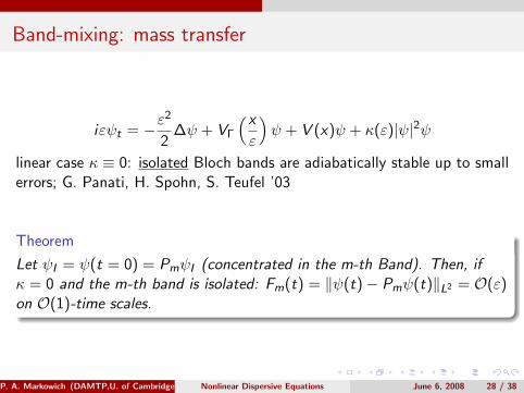
Band-mixing: mass transfer
iεψt = −ε2
2∆ψ + VΓ
(x
ε
)ψ + V (x)ψ + κ(ε)|ψ|2ψ
linear case κ ≡ 0: isolated Bloch bands are adiabatically stable up to smallerrors; G. Panati, H. Spohn, S. Teufel ’03
Theorem
Let ψI = ψ(t = 0) = PmψI (concentrated in the m-th Band). Then, ifκ = 0 and the m-th band is isolated: Fm(t) = ‖ψ(t)− Pmψ(t)‖L2 = O(ε)on O(1)-time scales.
P. A. Markowich (DAMTP,U. of Cambridge) Nonlinear Dispersive Equations June 6, 2008 28 / 38
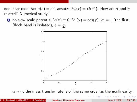
nonlinear case: set κ(ε) = εα, ansatz: Fm(t) = O(εγ). How are α and γrelated? Numerical study!
1 no slow scale potential V (x) ≡ 0, VΓ(y) = cos(y), m = 1 (the firstBloch band is isolated), ε = 1
32
α ≈ γ, the mass transfer rate is of the same order as the nonlinearity.
P. A. Markowich (DAMTP,U. of Cambridge) Nonlinear Dispersive Equations June 6, 2008 29 / 38
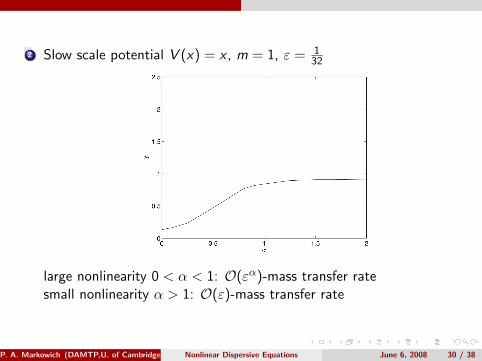
2 Slow scale potential V (x) = x , m = 1, ε = 132
large nonlinearity 0 < α < 1: O(εα)-mass transfer ratesmall nonlinearity α > 1: O(ε)-mass transfer rate
P. A. Markowich (DAMTP,U. of Cambridge) Nonlinear Dispersive Equations June 6, 2008 30 / 38
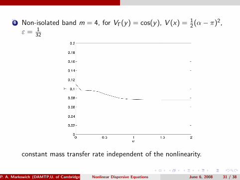
3 Non-isolated band m = 4, for VΓ(y) = cos(y), V (x) = 12 (α− π)2,
ε = 132
constant mass transfer rate independent of the nonlinearity.
P. A. Markowich (DAMTP,U. of Cambridge) Nonlinear Dispersive Equations June 6, 2008 31 / 38
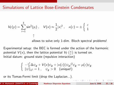
Simulations of Lattice Bose-Einstein Condensates
VΓ(y) =3∑
i=1
sin2(yi ) , V (x) ≈ 1
2|x |2 , κ(ε) = ±
{ε1
↑allows to solve only 1-dim. Bloch spectral problems!
Experimental setup: the BEC is formed under the action of the harmonicpotential V (x), then the lattice potential VΓ
(xε
)is turned on.
Initial datum: ground state (repulsive interaction){− ε2
2 ∆ψg + V (x)ψg + |κ(ε)||ψg |2ψg = µ(ε)ψg
‖ψ‖L2 = 1 , ψg > 0 (unique!)
or its Tomas-Fermi limit (drop the Laplacian...).
P. A. Markowich (DAMTP,U. of Cambridge) Nonlinear Dispersive Equations June 6, 2008 32 / 38
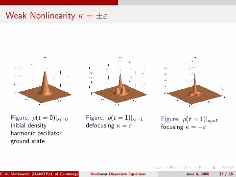
Weak Nonlinearity κ = ±ε
Figure: ρ(t = 0)|x3=0
initial densityharmonic oscillatorground state
Figure: ρ(t = 1)|x3=1
defocusing κ = εFigure: ρ(t = 1)|x3=1
focusing κ = −ε
P. A. Markowich (DAMTP,U. of Cambridge) Nonlinear Dispersive Equations June 6, 2008 33 / 38
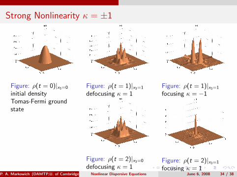
Strong Nonlinearity κ = ±1
Figure: ρ(t = 0)|x3=0
initial densityTomas-Fermi groundstate
Figure: ρ(t = 1)|x3=1
defocusing κ = 1Figure: ρ(t = 1)|x3=1
focusing κ = −1
Figure: ρ(t = 2)|x3=0
defocusing κ = 1Figure: ρ(t = 2)|x3=1
focusing κ = 1P. A. Markowich (DAMTP,U. of Cambridge) Nonlinear Dispersive Equations June 6, 2008 34 / 38
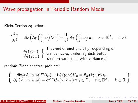
Wave propagation in Periodic Random Media
Klein-Gordon equation:
∂2u
∂t2= div
(AΓ
(x
ε;ω)∇u)− 1
ε2WΓ
(x
ε;ω)
u , x ∈ Rd , t > 0
AΓ(y ;ω)WΓ(y ;ω)
} Γ-periodic functions of y , depending ona mean-zero, uniformly distributed,random variable ω with variance σ
random Bloch-spectral problem:{− divy (AΓ(y ;ω)∇Um) + WΓ(y ;ω)Um = Em(k ;ω)2Um
Um(y + γ, k ;ω) = e ik·γUm(y , k ;ω) ∀ γ ∈ Γ , y ∈ Rd , k ∈ B
}
P. A. Markowich (DAMTP,U. of Cambridge) Nonlinear Dispersive Equations June 6, 2008 35 / 38
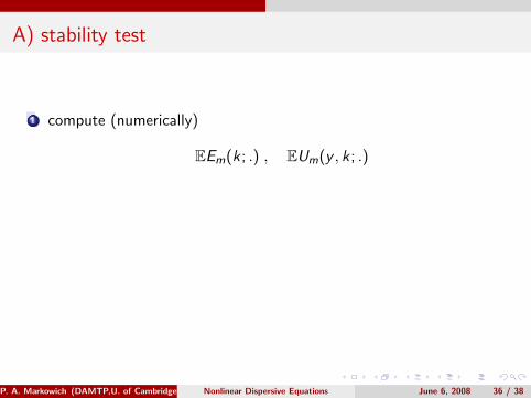
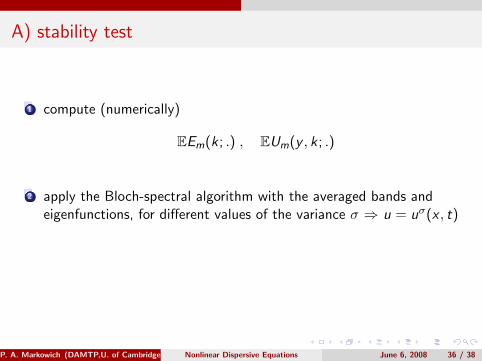
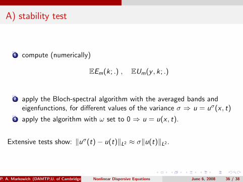
A) stability test
1 compute (numerically)
EEm(k; .) , EUm(y , k ; .)
2 apply the Bloch-spectral algorithm with the averaged bands andeigenfunctions, for different values of the variance σ ⇒ u = uσ(x , t)
3 apply the algorithm with ω set to 0 ⇒ u = u(x , t).
Extensive tests show: ‖uσ(t)− u(t)‖L2 ≈ σ‖u(t)‖L2 .
P. A. Markowich (DAMTP,U. of Cambridge) Nonlinear Dispersive Equations June 6, 2008 36 / 38
Numerical Evidence for Anderson Localisation
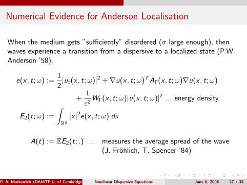
When the medium gets ”sufficiently” disordered (σ large enough), thenwaves experience a transition from a dispersive to a localized state (P.W.Anderson ’58).
e(x , t;ω) :=1
2|ut(x , t;ω)|2 +∇u(x , t;ω)T AΓ(x , t;ω)∇u(x , t;ω)
+1
ε2WΓ(x , t;ω)|u(x , t;ω)|2 ... energy density
E2(t;ω) :=
∫Rd
|x |2e(x , t;ω) dx
A(t) := EE2(t; .) ... measures the average spread of the wave(J. Frohlich, T. Spencer ’84)
P. A. Markowich (DAMTP,U. of Cambridge) Nonlinear Dispersive Equations June 6, 2008 37 / 38
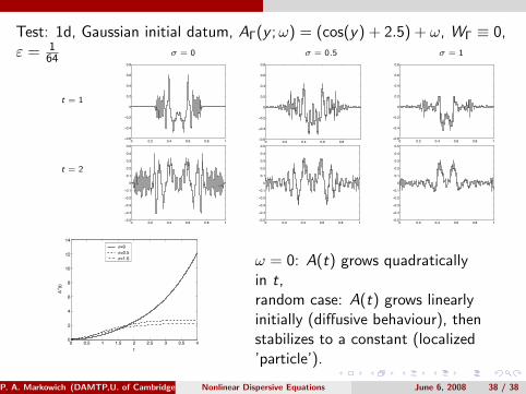
Test: 1d, Gaussian initial datum, AΓ(y ;ω) = (cos(y) + 2.5) + ω, WΓ ≡ 0,ε = 1
64
t = 1
σ = 0
0 0.2 0.4 0.6 0.8 1−0.6
−0.4
−0.2
0
0.2
0.4
0.6
0.8
σ = 0.5
0 0.2 0.4 0.6 0.8−0.6
−0.4
−0.2
0
0.2
0.4
0.6
0.8
σ = 1
0 0.2 0.4 0.6 0.8 1−0.6
−0.4
−0.2
0
0.2
0.4
0.6
0.8
t = 2
0 0.2 0.4 0.6 0.8 1−0.5
−0.4
−0.3
−0.2
−0.1
0
0.1
0.2
0.3
0.4
0.5
0 0.2 0.4 0.6 0.8 1−0.5
−0.4
−0.3
−0.2
−0.1
0
0.1
0.2
0.3
0.4
0.5
0 0.2 0.4 0.6 0.8 1−0.5
−0.4
−0.3
−0.2
−0.1
0
0.1
0.2
0.3
0.4
0.5
0 0.5 1 1.5 2 2.5 3 3.5 40
2
4
6
8
10
12
14
t
Aσ(t)
σ=0σ=0.5σ=1.0 ω = 0: A(t) grows quadratically
in t,random case: A(t) grows linearlyinitially (diffusive behaviour), thenstabilizes to a constant (localized’particle’).
P. A. Markowich (DAMTP,U. of Cambridge) Nonlinear Dispersive Equations June 6, 2008 38 / 38