Patrick Breheny April 21

OverdispersionPoisson regression for contingency tables

Poisson regression: Further topics

Patrick Breheny

April 21

Patrick Breheny BST 760: Advanced Regression


Quasi-likelihoodNegative binomial

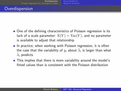
Overdispersion

One of the defining characteristics of Poisson regression is itslack of a scale parameter: E(Y ) = Var(Y ), and no parameteris available to adjust that relationship

In practice, when working with Poisson regression, it is oftenthe case that the variability of yi about λ̂i is larger than whatλ̂i predicts

This implies that there is more variability around the model’sfitted values than is consistent with the Poisson distribution




Overdispersion (cont’d)

The term for this phenomenon is overdispersion

Data for which this phenomenon manifests itself are oftencalled “overdispersed”, although as we will see, it is perhapsbetter to refer to the model as overdispersed, not the data

There are two common approaches to correcting foroverdispersion:

Quasi-likelihoodNegative binomial regression




Tinkering with the score

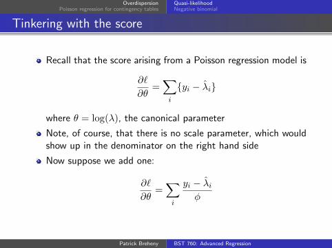
Recall that the score arising from a Poisson regression model is

∂`

∂θ=∑i

{yi − λ̂i}

where θ = log(λ), the canonical parameter

Note, of course, that there is no scale parameter, which wouldshow up in the denominator on the right hand side

Now suppose we add one:

∂`

∂θ=∑i

yi − λ̂iφ




Implications of our tinkering

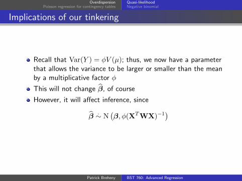
Recall that Var(Y ) = φV (µ); thus, we now have a parameterthat allows the variance to be larger or smaller than the meanby a multiplicative factor φ

This will not change β̂, of course

However, it will affect inference, since

β̂.∼ N

(β, φ(XTWX)−1

)




Quasi-likelihood

So what distribution is this, that gives rise to this score?

There isn’t one (at least, not one for which you can writedown the distribution in closed form)

This approach, where you modify the score directly and neveractually specify a distribution, is known as quasi-likelihood




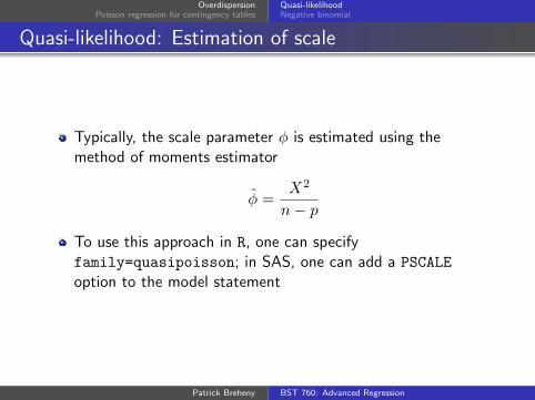
Quasi-likelihood: Estimation of scale

Typically, the scale parameter φ is estimated using themethod of moments estimator

φ̂ =X2

n− p

To use this approach in R, one can specifyfamily=quasipoisson; in SAS, one can add a PSCALE

option to the model statement




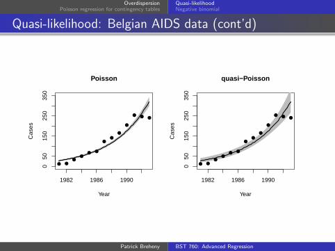
Quasi-likelihood: Belgian AIDS data

For our Belgian AIDS data, φ̂ = 6.7, implying that thevariance was nearly 7 times larger than that implied by thePoisson distribution

Again, the fit is the same

However, our standard errors are√6.7 ≈ 2.6 times larger




Quasi-likelihood: Belgian AIDS data (cont’d)

1982 1986 1990

050

150

250

350

Poisson

Year

Cas

es

● ●●

●● ●

●●

●

●

● ● ●

1982 1986 19900

5015

025

035

0

quasi−Poisson

Year

Cas

es● ●

●●

● ●

●●

●

●

● ● ●




Drawbacks of quasi-likelihood

The quasi-Poisson approach is attractive for several reasons,but its big drawback is that lacks a log-likelihood

This prevents you from using any of the likelihood-based toolswe have discussed for GLMs: likelihood ratio tests, AIC/BIC,deviance explained, deviance residuals

An alternative approach that allows all those maximumlikelihood tools is based on the negative binomial distribution




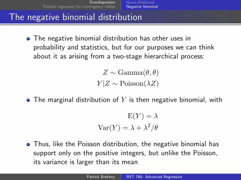
The negative binomial distribution

The negative binomial distribution has other uses inprobability and statistics, but for our purposes we can thinkabout it as arising from a two-stage hierarchical process:

Z ∼ Gamma(θ, θ)

Y |Z ∼ Poisson(λZ)

The marginal distribution of Y is then negative binomial, with

E(Y ) = λ

Var(Y ) = λ+ λ2/θ

Thus, like the Poisson distribution, the negative binomial hassupport only on the positive integers, but unlike the Poisson,its variance is larger than its mean




Negative binomial and exponential family

Note, however, that the negative binomial distribution is not amember of the exponential family

Thus, the theory and fitting procedures we have developed forGLMs do not directly apply here

For example, there is no “canonical link”; however, it iscustomary to employ a log link to make negative binomialregression look like Poisson regression




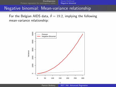
Negative binomial: Mean-variance relationship

For the Belgian AIDS data, θ̂ = 19.2, implying the followingmean-variance relationship:

0 50 100 150 200 250 300

010

0020

0030

0040

0050

00

λ

Var

ianc

e

PoissonNegative Binomial




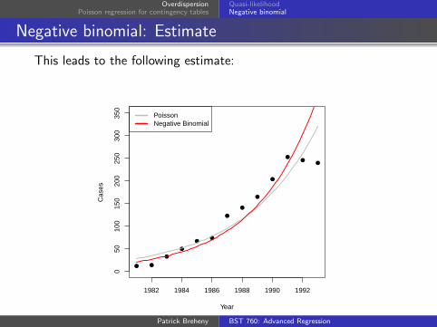
Negative binomial: Estimate

This leads to the following estimate:

● ●

●

●

●●

●

●

●

●

●●

●

1982 1984 1986 1988 1990 1992

050

100

150

200

250

300

350

Year

Cas

es

PoissonNegative Binomial




Remarks

By any reasonable assessment, the negative binomialestimates here are worse than the Poisson fit – and certainlydrastically worse than the quadratic Poisson model

However, its “goodness of fit” measures are much better

This is why I remarked earlier that it’s wrong to think of thedata as overdispersed – if the data show more variability thanthe model can explain, the most likely explanation is a badmodel

The quadratic Poisson fit shows no overdispersion (theresiduals are actually slightly “underdispersed”)




Remarks (cont’d)

The key concept here is that residual variance is caused bytwo things: random variation and systematic bias in the model

Many analysts have the mistaken view that quasi-Poisson ornegative binomial regression “automatically” fixes theoverdispersion problem

This is a dangerous misconception – systematic bias in themodel should take far greater priority than modeling therandom error

Quasi-Poisson or negative binomial should be thought of moreas a last resort to fixing overdispersion – the first step is fixingthe systematic component of the model



Poisson regression for contingency tables

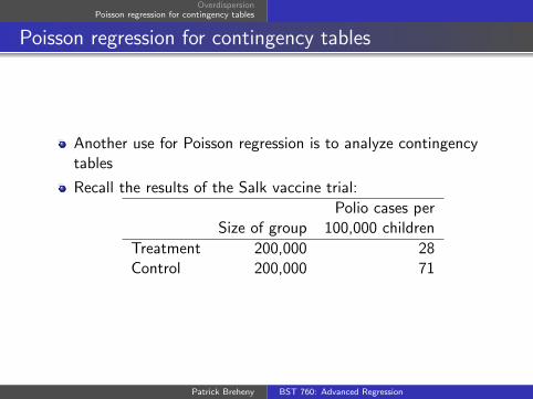
Another use for Poisson regression is to analyze contingencytables

Recall the results of the Salk vaccine trial:

Polio cases perSize of group 100,000 children

Treatment 200,000 28Control 200,000 71



Logistic vs. Poisson

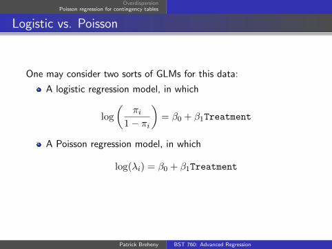
One may consider two sorts of GLMs for this data:

A logistic regression model, in which

log

(πi

1− πi

)= β0 + β1Treatment

A Poisson regression model, in which

log(λi) = β0 + β1Treatment



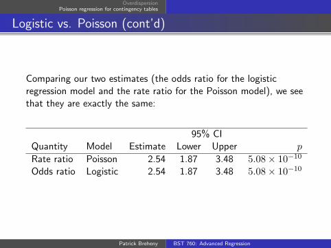
Logistic vs. Poisson (cont’d)

Comparing our two estimates (the odds ratio for the logisticregression model and the rate ratio for the Poisson model), we seethat they are exactly the same:

95% CIQuantity Model Estimate Lower Upper p

Rate ratio Poisson 2.54 1.87 3.48 5.08× 10−10

Odds ratio Logistic 2.54 1.87 3.48 5.08× 10−10



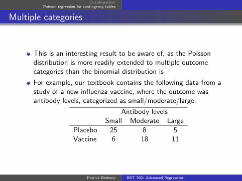
Multiple categories

This is an interesting result to be aware of, as the Poissondistribution is more readily extended to multiple outcomecategories than the binomial distribution is

For example, our textbook contains the following data from astudy of a new influenza vaccine, where the outcome wasantibody levels, categorized as small/moderate/large:

Antibody levelsSmall Moderate Large

Placebo 25 8 5Vaccine 6 18 11



Testing for association

We can model these six counts as Poisson random variableswith offset n0 = 38 for the placebo group and n1 = 35 for thevaccine group, then test the null hypothesis that thesmall/moderate/large rates are the same for the vaccine groupas they are for the placebo group

Assuming we parameterize the model in the usual way, thisamounts to a test of the interaction term between antibodylevels and group

A likelihood ratio test of the full model in which each cell hasits own Poisson rate vs. the restricted model in which therates are the same in each group points is highly significant(p = 0.00009), indicating that we are unlikely to have seensuch a large antibody response in the vaccine group due tochance alone



Remarks

In this case, we could just have used a χ2 or Fisher’s ExactTest to accomplish the same thing

The advantage of the Poisson model in general is that itallows us to build more complicated models with additionalexplanatory variables, and to model continuous variables usinglinear trends

In practice, these models become unwieldy rather quickly aswe try to add complexity

Next time, we’ll talk about ways to extend logistic regressionto the multi-category case


Patrick Breheny April 21

Documents

Transcript of Patrick Breheny April 21