Parametric estimation of a bivariate stable L´evy process
22
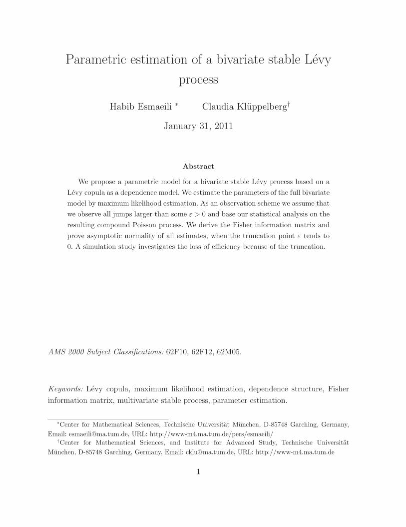
Parametric estimation of a bivariate stable L´ evy process Habib Esmaeili ∗ Claudia Kl¨ uppelberg † January 31, 2011 Abstract We propose a parametric model for a bivariate stable L´ evy process based on a L´ evy copula as a dependence model. We estimate the parameters of the full bivariate model by maximum likelihood estimation. As an observation scheme we assume that we observe all jumps larger than some ε> 0 and base our statistical analysis on the resulting compound Poisson process. We derive the Fisher information matrix and prove asymptotic normality of all estimates, when the truncation point ε tends to 0. A simulation study investigates the loss of efficiency because of the truncation. AMS 2000 Subject Classifications: 62F10, 62F12, 62M05. Keywords: L´ evy copula, maximum likelihood estimation, dependence structure, Fisher information matrix, multivariate stable process, parameter estimation. * Center for Mathematical Sciences, Technische Universit¨ at M¨ unchen, D-85748 Garching, Germany, Email: [email protected], URL: http://www-m4.ma.tum.de/pers/esmaeili/ † Center for Mathematical Sciences, and Institute for Advanced Study, Technische Universit¨ at M¨ unchen, D-85748 Garching, Germany, Email: [email protected], URL: http://www-m4.ma.tum.de 1
Transcript of Parametric estimation of a bivariate stable L´evy process
Parametric estimation of a bivariate stable Levy
process
Habib Esmaeili ∗ Claudia Kluppelberg†
January 31, 2011
Abstract
We propose a parametric model for a bivariate stable Levy process based on a
Levy copula as a dependence model. We estimate the parameters of the full bivariate
model by maximum likelihood estimation. As an observation scheme we assume that
we observe all jumps larger than some ε > 0 and base our statistical analysis on the
resulting compound Poisson process. We derive the Fisher information matrix and
prove asymptotic normality of all estimates, when the truncation point ε tends to
0. A simulation study investigates the loss of efficiency because of the truncation.
AMS 2000 Subject Classifications: 62F10, 62F12, 62M05.
Keywords: Levy copula, maximum likelihood estimation, dependence structure, Fisher
information matrix, multivariate stable process, parameter estimation.
∗Center for Mathematical Sciences, Technische Universitat Munchen, D-85748 Garching, Germany,
Email: [email protected], URL: http://www-m4.ma.tum.de/pers/esmaeili/†Center for Mathematical Sciences, and Institute for Advanced Study, Technische Universitat
Munchen, D-85748 Garching, Germany, Email: [email protected], URL: http://www-m4.ma.tum.de
1
1 Introduction
The problem of parameter estimation of one-dimensional stable Levy processes has been
investigated already in the seventies of the last century by Basawa and Brockwell [3, 4].
Starting with a subordinator model, they assumed that it is possible to observe n(ε) jumps
in a time interval [0, t], all larger than a certain small ε > 0. Based on this observation
scheme, they estimated the parameters by a maximum likelihood procedure, and investi-
gated the distributional limits of the MLEs for n(ε) → ∞, which in this model if either
t→ ∞ and/or ε→ 0.
The task of estimating multivariate stable processes is usually solved by estimating
the parameters of the marginal processes and the spectral measure separately; cf. Nolan,
Panorska and McCulloch [14] and Hopfner [10] and references therein.
The rather recent modelling of multivariate Levy processes by their marginal processes
and a Levy copula for the dependence structure (cf. Cont and Tankov [6], Kallsen and
Tankov [12], and Eder and Kluppelberg [7]) allows for the construction of new paramet-
ric models. This approach is similar to the representation of a multivariate distribution
function by its marginal distributions and a copula and is valid for all multivariate Levy
processes.
Moreover, various estimation methods of the parameters of the marginal processes
and the dependence structure either together or separately can be applied. Obviously, it
is more efficient to estimate all parameters of a model in one go, but often the attempt fails.
Problems may occur because of the complexity of the numerical optimization involved to
obtain the MLEs of the parameters or, given the estimates, their asymptotic properties
are not clear concerning their asymptotic covariance structure.
This is an important point in the context of Levy processes, since these properties
may depend on the observation scheme. In reality it is usually not possible to observe
the continuous-time sample path, but it may be possible to observe all jumps larger than
ε as in the one-dimensional problem studied by Basawa and Brockwell [4]. For a stable
subordinator we obtain asymptotic normality for such an observation scheme, provided
that n(ε) → ∞, equivalently ε → 0. In a general multivariate model this is not clear at
all, in particular, for the dependence parameters.
With this paper we want to start an investigation concerning statistical estimation
of multivariate Levy processes in a parametric framework. In a certain sense the present
paper is a follow-up of Esmaeili and Kluppelberg [8], where we concentrated on parametric
estimation of multivariate compound Poisson processes.
Since our observation scheme involves only jumps larger than ε, the observed process
is a multivariate compound Poisson process. But in contrast to [8], we now assume that
the Levy process has infinite Levy measure and we investigate asymptotic normality also
2
for ε→ 0.
Our paper is organised as follows. In Section 2 we present some basic facts about Levy
copulas and recall the estimation procedure as presented in Basawa and Brockwell [3, 4]
for one-dimensional α-stable subordinators in Section 3. Section 4 contains the theoretical
body of our new results. In Section 4.1 we present the small jumps truncation and its
consequences for the Levy copula; Section 4.2 presents the maximum likelihood estimation
for the α-stable Clayton subordinator, including an explicit calculation of the Fisher
information matrix, which ensures joint asymptotic normality of all estimates. Section 5
presents a simulation study and Section 6 concludes and gives an outlook to further work.
2 Levy processes and Levy copulas
Let S = (S(t))t≥0 be a Levy process with values in Rd defined on a filtered probability
space (Ω, (Ft)t≥0,F ,P); i.e S has independent and stationary increments, and we assume
that it has cadlag sample paths. For each t > 0, the random variable S(t) has an infinitely
divisible distribution, whose characteristic function has a Levy-Khintchine representation:
E[ei(z,Xt)] = exp
t
(i(γ, z) − 1
2z⊤Az +
∫
Rd
(ei(z,x) − 1 − i(z, x)1|x|≤1
)Π(dx)
), z ∈ R
d ,
where (·, ·) denotes the inner product in Rd, γ ∈ R
d and A is a symmetric nonnegative
definite d × d matrix. The Levy measure Π is a measure on Rd satisfying Π(0) = 0
and∫
Rd\0min1, |x|2Π(dx) < ∞. For every Levy process its distribution is defined by
(γ,A,Π), which is called the characteristic triplet. It is worth mentioning that the Levy
measure Π(B) for B ∈ B(Rd) is the expected number of jumps per unit time with size in
B.
Brownian motion is characterised by (0, A, 0) and Brownian motion with drift by
(γ,A, 0). Poisson processes and compound Poisson processes have characteristic triplet
(γ1, 0,Π). The class of Levy processes is very rich including prominent examples like sta-
ble processes, gamma processes, variance gamma processes, inverse Gaussian and normal
inverse Gaussian processes. Their applications reach from finance and insurance applica-
tions to the natural sciences and engineering. A particular role is played by subordinators,
which are Levy processes with increasing sample paths. Other important classes are spec-
trally one-sided Levy processes, which have only positive or only negative jumps.
We are concerned with dependence in the jump behaviour S, which we model by an
appropriate functional of the marginals of the Levy measure Π. Since, with the exception
of a compound Poisson model, all Levy measures have a singularity in 0, we follow Cont
and Tankov [6] and introduce a (survival) copula on the tail integral, which is called Levy
copula and, because of the singularity in 0, is defined for each quadrant separately; for
3
details we refer to Kallsen and Tankov [12] and to Eder and Kluppelberg [7] for a different
approach.
Throughout this paper we restrict the presentation to the positive cone Rd+, where
only common positive jumps in all component processes happen. To extend this theory
to general Levy processes is not difficult, but notationally involved.
We present the definition of the tail integral on the positive cone Rd+. For a spectrally
positive Levy process this characterises the jump behaviour completely.
Definition 2.1. Let Π be a Levy measure on Rd+. The tail integral is a function Π :
[0,∞]d → [0,∞] defined by
Π(x1, . . . , xd) =
Π([x1,∞) × · · · × [xd,∞)) , (x1, . . . , xd) ∈ [0,∞)d \ 00 , xi = ∞ for at least one i
∞ , (x1, . . . , xd) = 0.
The marginal tail integrals are defined analogously for i = 1, . . . , d as Πi(x) = Πi([x,∞))
for x ≥ 0.
Also the Levy copula is defined quadrantwise and characterises the dependence struc-
ture of a spectrally positive Levy process completely.
Definition 2.2. A d-dimensional positive Levy copula is a measure defining function
C : [0,∞]d → [0,∞] with margins Ck(u) = u for all u ∈ [0,∞] and k = 1, . . . , d.
The following theorem is a version of Sklar’s theorem for Levy processes with positive
jumps, proved in Tankov [17], Theorem 3.1; for the corresponding result for general Levy
processs we refer again to Kallsen and Tankov [12].
Theorem 2.3 (Sklar’s Theorem for Levy copulas). Let Π denote the tail integral of a
spectrally positive d-dimensional Levy process, whose components have Levy measures
Π1, . . . ,Πd. Then there exists a Levy copula C : [0,∞]d → [0,∞] such that for all
x1, x2, . . . , xd ∈ [0,∞]
Π(x1, . . . , xd) = C(Π1(x1), . . . ,Πd(xd)). (2.1)
If the marginal tail integrals are continuous, then this Levy copula is unique. Otherwise,
it is unique on RanΠ1 × · · · ×RanΠd.
Conversely, if C is a Levy copula and Π1, . . . ,Πd are marginal tail integrals of a spectrally
positive Levy process, then the relation (2.1) defines the tail integral of a d-dimensional
spectrally positive Levy process and Π1, . . . ,Πd are tail integrals of its components.
4
Remark 2.4. In the case of multivariate stable Levy processes the Levy copula carries the
same information as the spectral measure. By choosing a slightly different approach this
was shown in Eder and Kluppelberg [7]. Note, however, that the spectral measure restricts
to stable processes, whereas the Levy copula models the dependence for all Levy processes.
We are concerned with the estimation of the parameters of a multivariate Levy process
and assume for simplicity that we observe all jumps larger than ε > 0 of a subordinator.
This results in a compound Poisson process and we recall the following well-known results;
see e.g. Sato [16], Theorem 21.2 and Corollary 8.8.
Proposition 2.5. (a) A Levy process S in Rd is compound Poisson if and only if it has
a finite Levy measure Π with limx→0 Π(x) = λ, the intensity of the d-dimensional Poisson
process, and jump distribution F (dx) = λ−1Π(dx) for x ∈ Rd.
(b) Every Levy process is the limit of a sequence of compound Poisson processes.
3 Maximum likelihood estimation of the parameters
of a one-dimensional Levy process
3.1 Small jump truncation
With the understanding that the Levy measure can be decomposed in positive and neg-
ative jumps we restrict ourselves to subordinators.
Let S be a one-dimensional subordinator with unbounded Levy measure Π, without
drift or Gaussian part. For all t ≥ 0 its characteristic function has the representation
EeiuS(t) = etψ(u) for u ∈ R with
ψ(u) =
∫
0<x<ε
(eiux − 1
)Π(dx) +
∫
x≥ε
(eiux − 1
)Π(dx), u ∈ R , (3.1)
for arbitrary ε > 0. The last integral in (3.1) is the characteristic exponent of a compound
Poisson process with Poisson intensity λ(ε) ∈ (0,∞) and jump distribution function F (ε)
λ(ε) =
∫ ∞
ε
Π(dx) and F (ε)(dx) = Π(dx)/λ(ε) on [ε,∞).
As an observation scheme we assume that we observe the whole sample path of S
over a time interval [0, t], but that we only observe jumps of size larger than ε. Then
our observation scheme is equivalent to observing a compound Poisson process, say S(ε),
given in its marked point process representation as (T (ε)k , X
(ε)k ), k = 1, . . . , n(ε), where
n(ε) = n(ε)(t) = cardT (ε)k ∈ [0, t] : k ∈ N. We also assume that Π(dx) = ν(x; θ)dx
where θ is a vector of parameters of the Levy measure so that the density of X(ε)k is given
5
by f (ε)(x; θ) = ν(x, θ)/λ(ε) for x ≥ ε. The likelihood function of this compound Poisson
process is well-known, see e.g. Basawa and Prakasa Rao [5], and is given by
L(ε)(θ) = (λ(ε))n(ε)
e−λ(ε)t ×
n(ε)∏
i=1
f (ε)(xi, θ) = e−λ(ε)t ×
n(ε)∏
i=1
ν(xi; θ)1xi≥ε. (3.2)
3.2 Asymptotic behaviour of the MLEs
MLE is a well established estimation procedure and the asymptotic properties of the
estimators is well-known for iid data, but also for continuous-time stochastic processes,
see e.g. Kuchler and Sorensen [13] and references therein. However, this theory is usually
concerned about letting the observation time, i.e. t tends to infinity. We are more interested
in the case of fixed t and ε ↓ 0, and here there exist to our knowledge only some specific
results in the literature; see e.g. Basawa and Brockwell [3, 4] and Hopfner and Jacod [11].
We start with a general Levy process S and base the maximum likelihood estimation
on the jumps ∆Sv > ε for v ∈ [0, t]. The MLEs are, in fact, those obtained from the CPP
S(ε) as described in Section 3.1 above. Therefore, under some regularity conditions (see e.g.
Prakasa Rao [15], Section 3.11) the MLEs are consistent and asymptotically normal. In the
context of a compound Poisson process the asymptotic behavior of estimators is considered
for t → ∞. In our set-up, however, it is also relevant to consider the performance of
estimators as ε→ 0 with t fixed.
We investigate the asymptotic behavior of estimators for a stable Levy process as
n(ε) → ∞ and shall show that this covers the cases of t → ∞ as well as ε → 0. Asymp-
totic normality of the estimators has been derived in Basawa and Brockwell [3, 4]. For
comparison and later reference we summarize these results in some detail.
Example 3.1. [α-stable subordinator]
Let (S(t))t≥0 be a one dimensional α-stable subordinator with parameters c > 0 and
0 < α < 1, such that the tail integral Π(x) = cx−α for x > 0. Observing all jumps larger
than some ε > 0, the resulting CPP has intensity and jump size density
λ(ε) =
∫ ∞
ε
Π(dx) = cε−α , f (ε)(x) =Π(dx)/dx
λ(ε)= αεαx−1−α, x > ε.
If we observe n(ε) jumps larger than ε in [0, t], we estimate the intensity by λ(ε) = n(ε)
t.
Moreover, by (3.2) the loglikelihood function for θ = (α, log c) is given by
ℓ(α, c) = n(ε)(logα+ log c) − elog cε−αt− (1 + α)n(ε)∑
i=1
log xi .
6
We calculate the score functions as
∂ℓ
∂α=
n(ε)
α+ telog cε−α log ε−
n(ε)∑
i=1
log xi ,
∂ℓ
∂ log c= n(ε) − elog cε−αt
To obtain candidates for maxima we calculate
elog c =n(ε)
tε−α=λ(ε)
ε−α,
1
α= − t
n(ε)cε−α log ε+
1
n(ε)
n(ε)∑
i=1
log xi
=1
n(ε)
n(ε)∑
i=1
(log xi − log ε) + log ε(1 − λ(ε)
λ(ε)
).
Consequently, we have the maximum likelihood estimators
α =
1
n(ε)
n(ε)∑
i=1
(logX
(ε)i − log ε
)+ log ε
(1 − λ(ε)
λ(ε)
)−1
,
log c = log λ(ε) + α log ε .
Next we calculate the second derivatives as
∂2ℓ
∂α2= −n(ε) 1
α2− ctε−α(log ε)2 = −tcε−α
(λ(ε)
λ(ε)
1
α2+ (log ε)2
)
∂2ℓ
∂α ∂ log c= ctε−α log ε =
∂2ℓ
∂ log c∂α
∂2ℓ
∂(log c)2= −tcε−α .
Consequently, the Fisher information matrix is given by
I(ε)α,log c = tcε−α
(1α2 + (log ε)2 − log ε
− log ε 1
).
We calculate the determinant as det(I(ε)α,log c) = c2t2α−2ε−2α. Using Cramer’s rule of inver-
sion easily gives
(I(ε)α,log c)
−1 = (ct)−1εαα2
(1 log ε
log ε 1α2 + (log ε)2
).
7
We are interested in the asymptotic behaviour of the MLEs α and log c based on a fixed
time interval [0, t] and letting ε → 0. Note that we have to get the variance-covariance
matrix asymptotically independent of ε. Division of log c by log ε changes the matrix
I(ε)−1
α,log c into
(I(ε)
α, log clog ε
)−1 = t−1c−1εαα2
(1 1
1 1α2(log ε)2
+ 1
).
Since
√n(ε)
(λ(ε)
λ(ε)− 1
)=
√n(ε)
(n(ε)
tcε−α− 1
)d→ N(0, 1) , n(ε) → ∞ , (3.3)
and the regularity conditions of Section 3.11 of Prakasa Rao [15] are satisfied, classical
likelihood theory ensures that
√n(ε)
α− αlog c− log c
log ε
∼ AN
(0, α2
(1 1
1 1α2
1(log ε)2
+ 1
)), n(ε) → ∞ .
Consistency of λ(ε), obtained from (3.3), and a Taylor expansion of log x around c ensures
with Slutzky’s theorem that for ε→ 0,
√ctε−α/2
α
α− 1
1α log ε
(c
c− 1
)
d→ N
(0,
(1 1
1 1
))=
(N1
N2
),
where N1, N2 are standard normal random variables with Cov(N1, N2) = 1, which implies
that N1 = N2 = N . So the limit law is degenerate.
It has been shown in Jacod and Hopfner [11] that the natural parameterization is not
(c, α), but (λ(ε), α), which leads to asymptotically independent normal limits. Indeed, we
have
√n(ε)
α
α− 1
λ(ε)
λ(ε)− 1
d→ N
(0,
(1 0
0 1
)), n(ε) → ∞ ,
where n(ε) can again be replaced by tcε−α and the same result holds for t → ∞, equiva-
lently, ε→ 0.
8
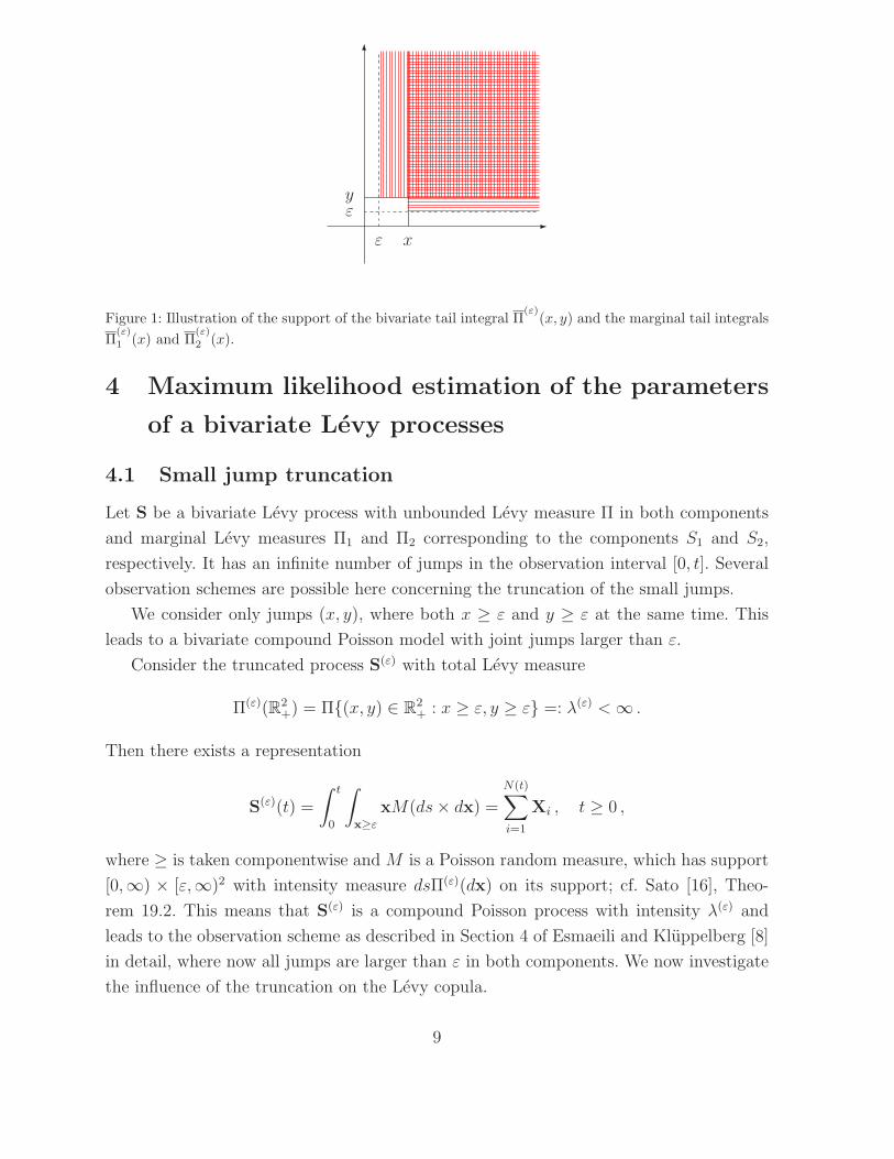
-
6
ε
ε x
y
Figure 1: Illustration of the support of the bivariate tail integral Π(ε)
(x, y) and the marginal tail integrals
Π(ε)
1 (x) and Π(ε)
2 (x).
4 Maximum likelihood estimation of the parameters
of a bivariate Levy processes
4.1 Small jump truncation
Let S be a bivariate Levy process with unbounded Levy measure Π in both components
and marginal Levy measures Π1 and Π2 corresponding to the components S1 and S2,
respectively. It has an infinite number of jumps in the observation interval [0, t]. Several
observation schemes are possible here concerning the truncation of the small jumps.
We consider only jumps (x, y), where both x ≥ ε and y ≥ ε at the same time. This
leads to a bivariate compound Poisson model with joint jumps larger than ε.
Consider the truncated process S(ε) with total Levy measure
Π(ε)(R2+) = Π(x, y) ∈ R
2+ : x ≥ ε, y ≥ ε =: λ(ε) <∞ .
Then there exists a representation
S(ε)(t) =
∫ t
0
∫
x≥ε
xM(ds× dx) =
N(t)∑
i=1
Xi , t ≥ 0 ,
where ≥ is taken componentwise and M is a Poisson random measure, which has support
[0,∞) × [ε,∞)2 with intensity measure dsΠ(ε)(dx) on its support; cf. Sato [16], Theo-
rem 19.2. This means that S(ε) is a compound Poisson process with intensity λ(ε) and
leads to the observation scheme as described in Section 4 of Esmaeili and Kluppelberg [8]
in detail, where now all jumps are larger than ε in both components. We now investigate
the influence of the truncation on the Levy copula.
9
Lemma 4.1. Let S be a bivariate Levy process with unbounded Levy measure Π concen-
trated on R2+ and Levy copula C, which is different from the independent Levy copula.
Consider only those jumps, which are larger than ε in both component processes. Then
the Levy copula of the resulting CPP is given by
C(ε)(u, v) = C(C←1 (u, λ
(ε)2 ),C←2 (λ
(ε)1 , v)), 0 < u, v ≤ λ(ε). (4.1)
where C←k , k = 1, 2 is the inverse of C with respect to the k-th argument, λ
(ε)k = Πk(ε), k =
1, 2, and λ(ε) = Π(ε, ε).
Proof. The marginal tail integrals of the CPP are given by
Π(ε)
1 (x) = Π(x, ε) = C(Π1(x),Π2(ε)) = C(Π1(x), λ(ε)2 ), x > ε,
Π(ε)
2 (y) = Π(ε, y) = C(Π1(ε),Π2(y)) = C(λ(ε)1 ,Π2(y)), y > ε,
(4.2)
whereas the bivariate tail integral is
Π(ε)
(x, y) = Π(x, y) = C(Π1(x),Π2(y)), x, y > ε. (4.3)
Denote by C(ε) the Levy copula of the CPP, and from (4.3) we have
C(ε)(Π
(ε)
1 (x),Π(ε)
2 (y)) = C(Π1(x),Π2(y)), x, y > ε.
Together with (4.2) this implies that
C(ε)(C(Π1(x), λ
(ε)2 ),C(λ
(ε)1 ,Π2(y))) = C(Π1(x),Π2(y)), x, y > ε.
Setting u := C(Π1(x), λ(ε)2 ) and v := C(λ
(ε)1 ,Π2(y)), we see that for x, y > ε
Π1(x) = C←1 (u, λ
(ε)2 ) and Π2(y) = C
←2 (λ
(ε)1 , v),
and, hence, for 0 < u, v ≤ λ(ε)
C(ε)(u, v) = C
(C←1 (u, λ
(ε)2 ),C←2 (λ
(ε)1 , v)
).
Proposition 4.2. Assume that the conditions of Lemma 4.1 hold. Then
limε→0
C(ε)(u, v) = C(u, v) , u, v > 0 .
10
Proof. Take arbitrary u, v > 0. Then there exists some ε > 0 such that 0 < u, v ≤ λ(ε).
Invoking the Lipschitz condition for Levy copula (Theorem 2.1, Barndorff-Nielsen and
Lindner [2])and (4.1), we have
|C(ε)(u, v) − C(u, v)| =∣∣∣C(C←1 (u, λ
(ε)2 ),C←2 (λ
(ε)1 , v)
)− C(u, v)
∣∣∣
≤∣∣∣C←1 (u, λ
(ε)2 ) − u
∣∣∣+∣∣∣C←2 (λ
(ε)1 , v) − v
∣∣∣ .
Since the Levy copula C has Lebesgue margins, i.e. C(u,∞) = u and C(∞, v) = v, we
have C←1 (u,∞) = u and C
←2 (∞, v) = v. This implies that
|C(ε)(u, v) − C(u, v)| ≤∣∣∣C←1 (u, λ
(ε)2 ) − C
←1 (u,∞)
∣∣∣+∣∣∣C←2 (λ
(ε)1 , v) − C
←2 (∞, v)
∣∣∣ .
The terms on the rhs tend to zero because the Levy measure is unbounded and limε→0 λ(ε)1 =
limε→0 λ(ε)2 = ∞.
Now we proceed as in Esmaeili and Kluppelberg [8] and use the same notation. Denote
by (x1, y1), . . . , (xn(ε) , yn(ε)) the observed jumps larger than ε in both components, i.e.
occurring at the same time during the observation interval [0, t]. Assume further that
the dependence structure of the process S = (S1, S2) is defined by a Levy copula C with
a parameter vector δ. We also assume that γ1 and γ2 are the parameter vectors of the
marginal Levy measures Π1 and Π2.
Using the notation νk(·) = λ(ε)k f
(ε)k (·) for the marginal Levy densities on (ε,∞) for
k = 1, 2 we can reformulate Theorem 4.1 of Esmaeili and Kluppelberg [8] as follows.
Theorem 4.3. Assume an observation scheme as above for a bivariate Levy process with
only non-negative jumps. Assume that γ1 and γ2 are the parameters of the marginal Levy
measures Π1 and Π2 with Levy densities ν1 and ν2, respectively, and a Levy copula C
with parameter vector δ. Assume further that ∂2
∂u∂vC(u, v; δ) exists for all (u, v) ∈ (0,∞)2,
which is the domain of C. Then the full likelihood of the bivariate CPP is given by
L(ε)(γ1, γ2, δ) = e−λ(ε)t
n(ε)∏
i=1
ν1(xi; γ1)ν2(yi; γ2)
∂2
∂u∂vC(u, v; δ)
∣∣∣∣u=Π1(xi;γ1),
v=Π2(yi;γ2)
(4.4)
where
λ(ε) =
∫ ∞
ε
∫ ∞
ε
Π(dx, dy) = C(Π1(ε; γ1),Π2(ε; γ2); δ).
4.2 Asymptotic behaviour of the MLEs of a bivariate stable
Clayton model
A spectrally positive Levy process is an α-stable subordinator if and only if 0 < α < 1
and there exists a finite measure ρ on the unit sphere Sd−1 := x ∈ Rd+ | ‖x‖ = 1 in R
d+
11

(for an arbitrary norm ‖ · ‖) such that the Levy measure
Π(B) =
∫
Sd−1
ρ(dξ)
∫ ∞
0
1B(rξ)dr
r1+α, B ∈ B(Rd
+) ,
(cf. Theorem 14.3(ii) and Example 21.7 in Sato [16]).
From Kallsen and Tankov [12], Theorem 4.6, it is known that a bivariate process is
α-stable if and only if it has α-stable marginal processes and a homogeneous Levy copula
of order 1; i.e. C(tu, tv) = t C(u, v). The Clayton Levy copula
C(u, v) =(u−δ + v−δ
)−1/δ
, u, v > 0 ,
is homogeneous of order 1. Hence it is a valid model to define a bivariate α-stable process.
Suppose S1 and S2 are two α-stable subordinators with same tail integrals
Πk(x) = cx−α , x > 0 , for k = 1, 2.
Assume further that S = (S1, S2) is a bivariate α-stable process with dependence structure
modeled by a Clayton Levy copula. The joint tail integral is then given by
Π(x, y) = C(Π1(x),Π2(y)) = c(xαδ + yαδ
)− 1δ , x, y > 0 . (4.5)
The bivariate Levy density is given by
ν(x, y) = c(1 + δ)α2(xy)αδ−1(xαδ + yαδ
)− 1δ−2, x, y > 0 , (4.6)
We assume the observation scheme as in Section 4.1. The Levy measure Π will be consid-
ered on the set [ε,∞) × [ε,∞) with jump intensity
λ(ε) = Π(ε, ε) = c(εαδ + εαδ
)− 1δ = c2−1/δε−α. (4.7)
and marginal tail integrals
Π(ε)
k (x) = c(xαδ + εαδ)−1/δ , k = 1, 2. (4.8)
Moreover, for k = 1, 2,
Π(ε)
k (ε) = c2−1/δε−α = λ(ε) ,
and
G(ε)
k (x) = P (X > x) = P (Y > x) =Π
(ε)
k (x)
λ(ε)
=[12
(1 +
(xε
)αδ)]−1/δ
, x > ε . (4.9)
12
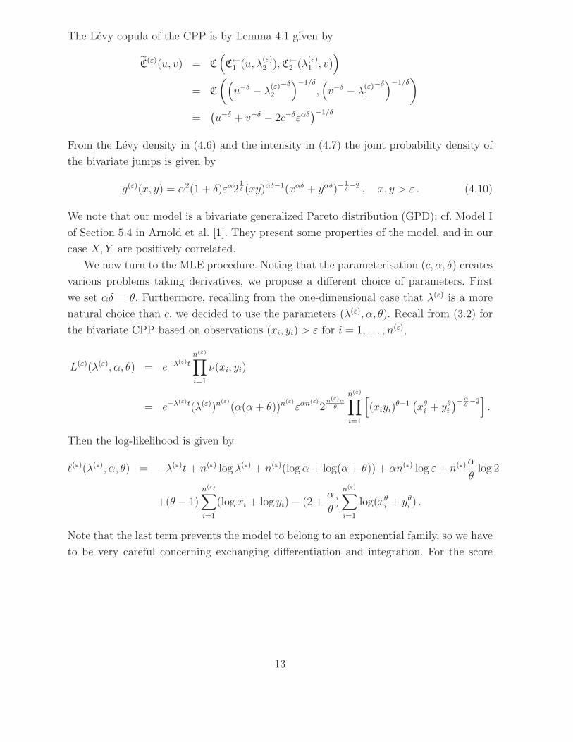
The Levy copula of the CPP is by Lemma 4.1 given by
C(ε)(u, v) = C
(C←1 (u, λ
(ε)2 ),C←2 (λ
(ε)1 , v)
)
= C
((u−δ − λ
(ε)2
−δ)−1/δ
,(v−δ − λ
(ε)1
−δ)−1/δ
)
=(u−δ + v−δ − 2c−δεαδ
)−1/δ
From the Levy density in (4.6) and the intensity in (4.7) the joint probability density of
the bivariate jumps is given by
g(ε)(x, y) = α2(1 + δ)εα21δ (xy)αδ−1(xαδ + yαδ)−
1δ−2 , x, y > ε . (4.10)
We note that our model is a bivariate generalized Pareto distribution (GPD); cf. Model I
of Section 5.4 in Arnold et al. [1]. They present some properties of the model, and in our
case X,Y are positively correlated.
We now turn to the MLE procedure. Noting that the parameterisation (c, α, δ) creates
various problems taking derivatives, we propose a different choice of parameters. First
we set αδ = θ. Furthermore, recalling from the one-dimensional case that λ(ε) is a more
natural choice than c, we decided to use the parameters (λ(ε), α, θ). Recall from (3.2) for
the bivariate CPP based on observations (xi, yi) > ε for i = 1, . . . , n(ε),
L(ε)(λ(ε), α, θ) = e−λ(ε)t
n(ε)∏
i=1
ν(xi, yi)
= e−λ(ε)t(λ(ε))n
(ε)
(α(α+ θ))n(ε)
εαn(ε)
2n(ε)α
θ
n(ε)∏
i=1
[(xiyi)
θ−1(xθi + yθi
)−αθ−2].
Then the log-likelihood is given by
ℓ(ε)(λ(ε), α, θ) = −λ(ε)t+ n(ε) log λ(ε) + n(ε)(logα+ log(α+ θ)) + αn(ε) log ε+ n(ε)α
θlog 2
+(θ − 1)n(ε)∑
i=1
(log xi + log yi) − (2 +α
θ)n(ε)∑
i=1
log(xθi + yθi ) .
Note that the last term prevents the model to belong to an exponential family, so we have
to be very careful concerning exchanging differentiation and integration. For the score
13
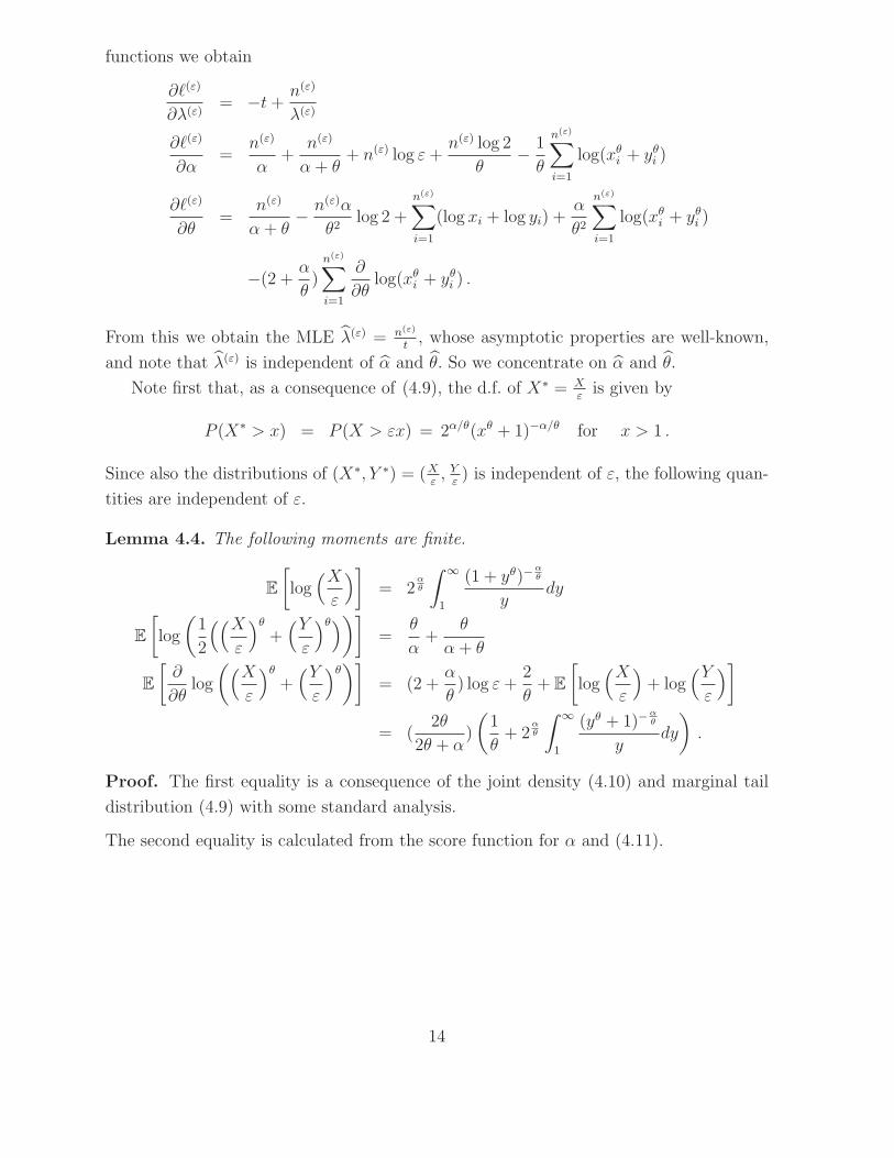
functions we obtain
∂ℓ(ε)
∂λ(ε)= −t+
n(ε)
λ(ε)
∂ℓ(ε)
∂α=
n(ε)
α+
n(ε)
α+ θ+ n(ε) log ε+
n(ε) log 2
θ− 1
θ
n(ε)∑
i=1
log(xθi + yθi )
∂ℓ(ε)
∂θ=
n(ε)
α+ θ− n(ε)α
θ2log 2 +
n(ε)∑
i=1
(log xi + log yi) +α
θ2
n(ε)∑
i=1
log(xθi + yθi )
−(2 +α
θ)n(ε)∑
i=1
∂
∂θlog(xθi + yθi ) .
From this we obtain the MLE λ(ε) = n(ε)
t, whose asymptotic properties are well-known,
and note that λ(ε) is independent of α and θ. So we concentrate on α and θ.
Note first that, as a consequence of (4.9), the d.f. of X∗ = Xε
is given by
P (X∗ > x) = P (X > εx) = 2α/θ(xθ + 1)−α/θ for x > 1 .
Since also the distributions of (X∗, Y ∗) = (Xε, Yε) is independent of ε, the following quan-
tities are independent of ε.
Lemma 4.4. The following moments are finite.
E
[log(Xε
)]= 2
αθ
∫ ∞
1
(1 + yθ)−αθ
ydy
E
[log
(1
2
((Xε
)θ+(Yε
)θ))]=
θ
α+
θ
α+ θ
E
[∂
∂θlog
((Xε
)θ+(Yε
)θ)]= (2 +
α
θ) log ε+
2
θ+ E
[log(Xε
)+ log
(Yε
)]
= (2θ
2θ + α)
(1
θ+ 2
αθ
∫ ∞
1
(yθ + 1)−αθ
ydy
).
Proof. The first equality is a consequence of the joint density (4.10) and marginal tail
distribution (4.9) with some standard analysis.
The second equality is calculated from the score function for α and (4.11).
14
For the last identity we calculate
(2 +α
θ)E
[∂
∂θlog(Xθ + Y θ)
]
=1
α+ θ− α
θ2log 2 + E [logX + log Y ] +
α
θ2E[log(Xθ + Y θ)
]
=1
α+ θ− α
θ2log 2 + E [logX + log Y ] +
α
θ2(θ log ε+
θ
α+
θ
α+ θ+ log 2)
=1
α+ θ(1 +
α
θ) + E [logX + log Y ] +
1
θ+α
θlog ε
= E [logX + log Y ] +2
θ+α
θlog ε
= (2 +α
θ) log ε+
2
θ+ 2
αθ+1
∫ ∞
1
(yθ + 1)−αθ
ydy .
The following is a first step for calculating the Fisher information matrix.
Lemma 4.5. For all ε > 0,
E[∂ℓ(ε)∂α
]= E
[∂ℓ(ε)∂θ
]= 0. (4.11)
Proof. We show the result for the partial derivative with respect to α, where we use a
dominated convergence argument. Since derivatives are local objects, it suffices to show
that for each α0 ∈ (0, 1) there exist a ξ > 0 such that for all α in a neighbourhood of α0,
given by Nξ(α0) := α ∈ (0, 1) : 0 < α0 − ξ ≤ α ≤ α0 + ξ < 1 there exists a dominating
integrable function, independent of α. We obtain
∣∣∣∣∂ℓ(ε)
∂α
∣∣∣∣ ≤ n(ε)
α0 − ξ+
n(ε)
α0 − ξ + θ+ n(ε) log ε+
n(ε) log 2
θ+
1
θ
n(ε)∑
i=1
∣∣∣ log(xθi + yθi )∣∣∣.
The right-hand side is integrable by Lemma 4.4, which can be seen by multiplying and
dividing the xi and yi by ε and using the second identity of Lemma 4.4.
The proof for the partial derivative with respect to θ is similar, invoking Lemma 4.4.
15

Next we calculate the second derivatives
∂2ℓ(ε)
∂α2= n(ε)
(− 1
α2− 1
(α+ θ)2
)
∂2ℓ(ε)
∂α∂θ= n(ε)
(− 1
(α+ θ)2− 1
θ2log 2
)− 1
θ
n(ε)∑
i=1
∂
∂θlog(xθi + yθi ) +
1
θ2
n(ε)∑
i=1
log(xθi + yθi )
∂2ℓ(ε)
∂θ∂α=
∂2ℓ(ε)
∂α∂θ
∂2ℓ(ε)
∂θ2= −n(ε)
(1
(α+ θ)2− 2α
θ3log 2
)− 2α
θ3
n(ε)∑
i=1
log(xθi + yθi ) +2α
θ2
n(ε)∑
i=1
∂
∂θlog(xθi + yθi )
−(2 +α
θ)n(ε)∑
i=1
∂2
∂θ2log(xθi + yθi ).
In order to calculate the Fisher information matrix we invoke Lemma 4.4. The compo-
nents of the Fisher information matrix are then given by
i11 = E
[− ∂2
∂α2ℓ(ε)]
= λ(ε)t
[1
α2+
1
(α+ θ)2
]
=: λ(ε)i11 t
i12 = i21 = E
[− ∂2
∂α∂θℓ(ε)]
= λ(ε)t
[1
(α+ θ)2− 1
αθ− 1
θ(α+ θ)+
1
θE
[∂
∂θlog
((Xε
)θ+(Yε
)θ)]]
= λ(ε)t
[1
(α+ θ)2+
2
θ(2θ + α)− 1
αθ− 1
θ(α+ θ)+
2α/θ+1
2θ + α
∫ ∞
1
(1 + uθ)−αθ
udu
]
=: λ(ε)i12 t = λ(ε)21 i12 t
i22 = E
[− ∂2
∂θ2ℓ(ε)]
= λ(ε)t
[1
(α+ θ)2− 2α log 2
θ3+
2α
θ3E(log(Xθ + Y θ)
)
−2α
θ2E
(∂
∂θlog(Xθ + Y θ)
)+ (
α
θ+ 2)E
(∂2
∂θ2log(Xθ + Y θ)
)]
= λ(ε)t
[1
(α+ θ)2+
2
θ2+
2α
θ2(α+ θ)− 4α
θ2(α+ 2θ)− α2α/θ+2
θ(2θ + α)
∫ ∞
1
(uθ + 1)−α/θ
udu
+(α
θ+ 2)g(α, θ)
]
=: λ(ε)i22 t ,
where
g(α, θ) := E
[∂2
∂θ2log(Xθ + Y θ)
]= E
[∂2
∂θ2log
((Xε
)θ+(Yε
)θ)]
16
does not depend on ε. This implies in particular that all ikl are independent of ε. Conse-
quently, the Fisher information matrix is given by
I(ε)α,θ = λ(ε)t
(i11 i12
i12 i22
).
Recall the asymptotic normality of the estimated parameters in the one-dimensional case
of Example 3.1. In our bivariate model we have additionally to those parameters the
dependence parameter θ. This means that we have to check the regularity conditions (A1)-
(A4) in Section 3.11 of Prakasa Rao [15] for this model. (A1) and (A2) are differentiability
conditions, which are satisfied. As a prerequisite for (A3) and (A4) we need to show
invertibility of the Fisher information matrix I(ε)α,θ, which we are not able to do analytically.
A numerical study for a large number of values for α and θ, however, always gave a positive
determinant, indicating that the inverse indeed exists. Since the Fisher information matrix
depends on t only by the common factor, it is not difficult to convince ourselves that also
(A3) and (A4) are satisfied. Hence, classical likelihood theory applies and ensures that
√n(ε)
(α− α
θ − θ
)∼ AN
0,
(i11 i12
i12 i22
)−1 , n(ε) → ∞ .
As in the one-dimensional case, we use the consistency result in (3.3) and Slutzky’s the-
orem, which gives for n(ε) → ∞, equivalently, ε→ 0,
√c2−α/θε−αt
(α− α
θ − θ
)d→ N
0,
(i11 i12
i12 i22
)−1 .
In reality the parameters are estimated from the data and plugged into the rate and the
ikl. Moreover, the unknown expectations in the Fisher information matrix have to be
either numerically calculated by the corresponding integrals or estimated by Monte Carlo
simulation. In Section 5 we shall perform a simulation study and also present an example
of the covariance matrix for some specific choice of parameters.
Before this we want to come back to our change of parameters and, in particular, want
to discuss estimation of the parameter c of the stable margins. From (3.3) and the fact
that λ(ε), α and θ are consistent, we know that for n(ε) → ∞,
c := λ(ε)2bα/bθεbα
is a consistent estimator of c.
We calculate as follows
log c = log λ(ε) +α
θlog 2 + α log ε
= logλ(ε)
λ(ε)+ log c− α
θlog 2 − α log ε+
α
θlog 2 + α log ε .
17
Consistency of λ(ε) implies that
log c− log c = oP (1) + (α− α) log ε+( αθ− α
θ
)log 2
= oP (1) + (α− α) log ε+(1
θ− 1
θ
)α log 2 + (α− α)
log 2
θ
= oP (1) + (α− α) log ε+(θθ− 1)αθ
log 2
+(α− α)log 2
θ(1 + oP (1)) ,
where we have used the consistency of α and θ. This implies for ε→ 0,
log c− log c
log ε= (α− α)(1 + oP (1)) .
Consequently, analogously to the one-dimensional case, we obtain the following result.
Theorem 4.6. Let (c, α, θ) denote the MLEs of the bivariate α-stable Clayton subordina-
tor. Then as ε→ 0,
√c2−α/θε−αt
log c− log c
log εα− α
θ − θ
d→
N1
N1
N2
, ε→ 0 ,
where Cov(N1, N2) =
(i11 i12
i12 i22
)−1
is independent of ε.
Obviously, we can do all again a Taylor expansion to obtain the limit law for c instead
of log c as in the one-dimensional case.
5 Simulation study for a bivariate α-stable Clayton
subordinator
We start generating data from a bivariate α-stable Clayton subordinator over a time
span [0, t], where we choose t = 1 for simplicity. Recall that our observation scheme
introduced in Section 4.1. assumes that from the α-stable Clayton subordinator we only
observe bivariate jumps larger than ε. Obviously, we cannot simulate a trajectory of a
stable process, since we are restricted to the simulation of a finite number of jumps. For
simulation purpose we choose a threshold ξ (which should be much smaller than ε) and
simulate jumps larger than ξ in one component, and arbitrary in the second component.
To this end we invoke Algorithm 6.15 in Cont and Tankov [6].
18
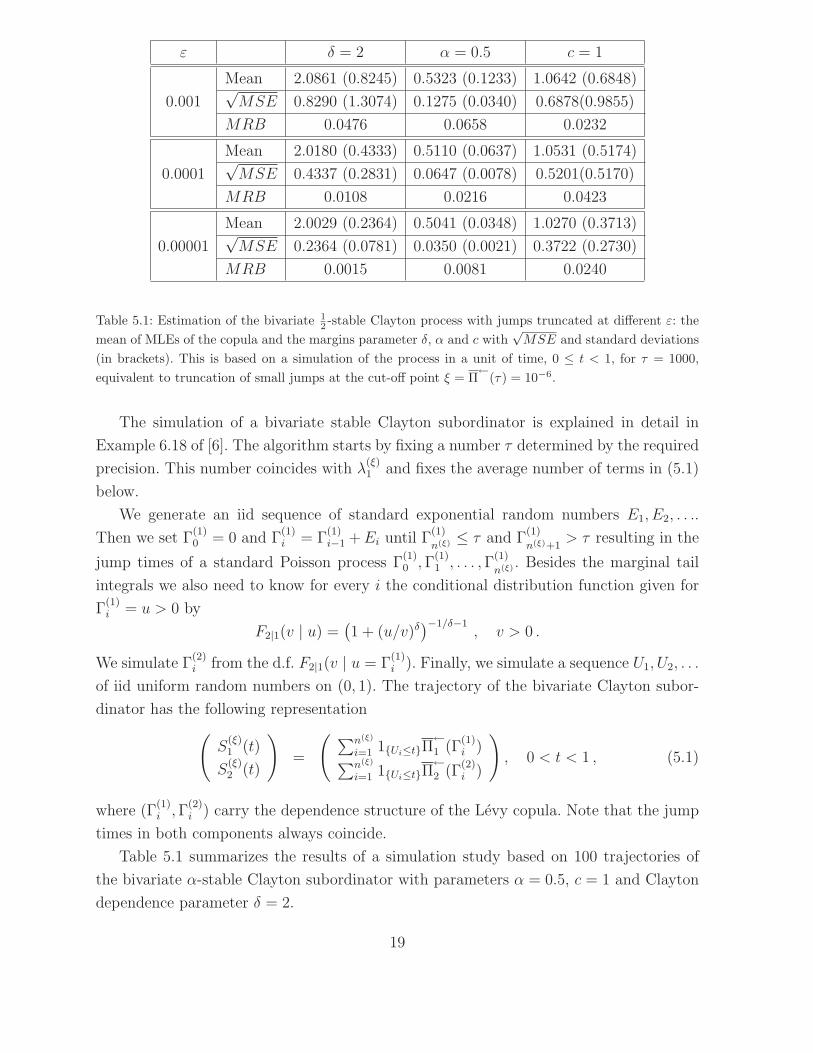
ε δ = 2 α = 0.5 c = 1
Mean 2.0861 (0.8245) 0.5323 (0.1233) 1.0642 (0.6848)
0.001√MSE 0.8290 (1.3074) 0.1275 (0.0340) 0.6878(0.9855)
MRB 0.0476 0.0658 0.0232
Mean 2.0180 (0.4333) 0.5110 (0.0637) 1.0531 (0.5174)
0.0001√MSE 0.4337 (0.2831) 0.0647 (0.0078) 0.5201(0.5170)
MRB 0.0108 0.0216 0.0423
Mean 2.0029 (0.2364) 0.5041 (0.0348) 1.0270 (0.3713)
0.00001√MSE 0.2364 (0.0781) 0.0350 (0.0021) 0.3722 (0.2730)
MRB 0.0015 0.0081 0.0240
Table 5.1: Estimation of the bivariate 12 -stable Clayton process with jumps truncated at different ε: the
mean of MLEs of the copula and the margins parameter δ, α and c with√
MSE and standard deviations
(in brackets). This is based on a simulation of the process in a unit of time, 0 ≤ t < 1, for τ = 1000,
equivalent to truncation of small jumps at the cut-off point ξ = Π←
(τ) = 10−6.
The simulation of a bivariate stable Clayton subordinator is explained in detail in
Example 6.18 of [6]. The algorithm starts by fixing a number τ determined by the required
precision. This number coincides with λ(ξ)1 and fixes the average number of terms in (5.1)
below.
We generate an iid sequence of standard exponential random numbers E1, E2, . . ..
Then we set Γ(1)0 = 0 and Γ
(1)i = Γ
(1)i−1 +Ei until Γ
(1)
n(ξ) ≤ τ and Γ(1)
n(ξ)+1> τ resulting in the
jump times of a standard Poisson process Γ(1)0 ,Γ
(1)1 , . . . ,Γ
(1)
n(ξ) . Besides the marginal tail
integrals we also need to know for every i the conditional distribution function given for
Γ(1)i = u > 0 by
F2|1(v | u) =(1 + (u/v)δ
)−1/δ−1, v > 0 .
We simulate Γ(2)i from the d.f. F2|1(v | u = Γ
(1)i ). Finally, we simulate a sequence U1, U2, . . .
of iid uniform random numbers on (0, 1). The trajectory of the bivariate Clayton subor-
dinator has the following representation
(S
(ξ)1 (t)
S(ξ)2 (t)
)=
( ∑n(ξ)
i=1 1Ui≤tΠ←
1 (Γ(1)i )
∑n(ξ)
i=1 1Ui≤tΠ←
2 (Γ(2)i )
), 0 < t < 1 , (5.1)
where (Γ(1)i ,Γ
(2)i ) carry the dependence structure of the Levy copula. Note that the jump
times in both components always coincide.
Table 5.1 summarizes the results of a simulation study based on 100 trajectories of
the bivariate α-stable Clayton subordinator with parameters α = 0.5, c = 1 and Clayton
dependence parameter δ = 2.
19
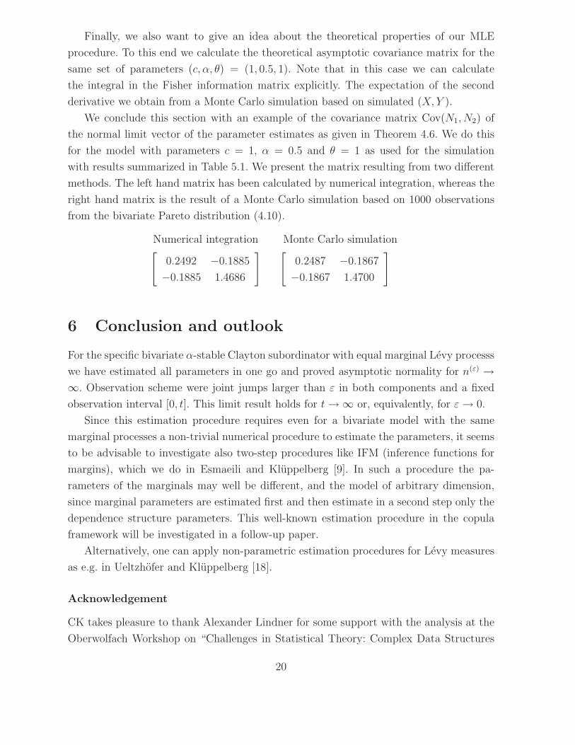
Finally, we also want to give an idea about the theoretical properties of our MLE
procedure. To this end we calculate the theoretical asymptotic covariance matrix for the
same set of parameters (c, α, θ) = (1, 0.5, 1). Note that in this case we can calculate
the integral in the Fisher information matrix explicitly. The expectation of the second
derivative we obtain from a Monte Carlo simulation based on simulated (X,Y ).
We conclude this section with an example of the covariance matrix Cov(N1, N2) of
the normal limit vector of the parameter estimates as given in Theorem 4.6. We do this
for the model with parameters c = 1, α = 0.5 and θ = 1 as used for the simulation
with results summarized in Table 5.1. We present the matrix resulting from two different
methods. The left hand matrix has been calculated by numerical integration, whereas the
right hand matrix is the result of a Monte Carlo simulation based on 1000 observations
from the bivariate Pareto distribution (4.10).
Numerical integration Monte Carlo simulation[
0.2492 −0.1885
−0.1885 1.4686
] [0.2487 −0.1867
−0.1867 1.4700
]
6 Conclusion and outlook
For the specific bivariate α-stable Clayton subordinator with equal marginal Levy processs
we have estimated all parameters in one go and proved asymptotic normality for n(ε) →∞. Observation scheme were joint jumps larger than ε in both components and a fixed
observation interval [0, t]. This limit result holds for t→ ∞ or, equivalently, for ε→ 0.
Since this estimation procedure requires even for a bivariate model with the same
marginal processes a non-trivial numerical procedure to estimate the parameters, it seems
to be advisable to investigate also two-step procedures like IFM (inference functions for
margins), which we do in Esmaeili and Kluppelberg [9]. In such a procedure the pa-
rameters of the marginals may well be different, and the model of arbitrary dimension,
since marginal parameters are estimated first and then estimate in a second step only the
dependence structure parameters. This well-known estimation procedure in the copula
framework will be investigated in a follow-up paper.
Alternatively, one can apply non-parametric estimation procedures for Levy measures
as e.g. in Ueltzhofer and Kluppelberg [18].
Acknowledgement
CK takes pleasure to thank Alexander Lindner for some support with the analysis at the
Oberwolfach Workshop on “Challenges in Statistical Theory: Complex Data Structures
20

and Algorithmic Optimization”.
References
[1] Arnold, B.C., Castillo, E. and Sarabia, J.M. (1999) Conditional Specification of Sta-
tistical Models. Springer, New York.
[2] Barndorff-Nielsen, O. and Lindner, A. (2007) Levy copulas: dynamics and transforms
of Upsilon type. Scand. J. Stat. 34, No. 2, 298-316(19).
[3] Basawa, I.V. and Brockwell, P.J. (1978) Inference for gamma and stable processes.
Biometrika 65, No. 1, 129-133.
[4] Basawa, I.V. and Brockwell, P.J. (1980) A note on estimation for gamma and stable
processes. Biometrika 67, No. 1, 234-236.
[5] Basawa, I.V. and Prakasa Rao, B.L.S. (1980) Statistical Inference for Stochastic Pro-
cesses. Academic Press, New York.
[6] Cont, R. and Tankov, P. (2004) Financial Modelling with Jump Processes. Chapman
& Hall/CRC, Boca Raton.
[7] Eder, I. and Kluppelberg, C. (2009) Pareto Levy measures and multivariate regular
variation. Submitted for publication.
[8] Esmaeili, H. and Kluppelberg, C. (2010) Parameter estimation of a bivariate com-
pound Poisson process. Insurance: Mathematics and Economics 47, 224-233.
[9] Esmaeili, H. and Kluppelberg, C. (2010) Two-step estimation of a multivariate Levy
process. Submitted for publication.
[10] Hopfner, R. (1999) On statistical models for d-dimensional stable processes, and some
generalisations. Scand. J. Stat. 26, 611-620.
[11] Hopfner, R. and Jacod, J. (1994) Some remarks on the joint estimation of the index
and the scale parameter for stable processes. In: Mandl, P. and Huskova, M. (Eds.)
Asymptotic Statistics. Proceedings of the Fifth Prague Symposium 1993, pp. 273-284.
Physica Verlag, Heidelberg.
[12] Kallsen, J. and Tankov, P. (2006) Characterization of dependence of multidimentional
Levy processes using Levy copulas. J. Mult. Anal. 97, 1551-1572.
21
[13] Kuchler, U. and Sørensen, M. (1997) Exponential Families of Stochastic Processes.
Springer, New York.
[14] Nolan, J.P., Panorska, A. and McCulloch, J.H. (2001) Estimation of stable spectral
measures Mathematical and Computer Modelling 34, 1113-1122.
[15] Prakasa Rao, B.L.S (1987) Asymptotic Theory of Statistical Inference. Wiley, New
York.
[16] Sato, K.-I. (1999) Levy Processes and Infinitely Divisible Distributions. Cambridge
University Press, Cambridge.
[17] Tankov, P. (2003) Dependence structure of spectrally positive multidimentional Levy
processes. Available at http://www.camp.polytechnique.fr/
[18] Ueltzhofer, F. and Kluppelberg, C. (2010) An oracle inequality for penalised projec-
tion estimation of Levy densities from high-frequency observations. Submitted for
publication.
22