Introduction to the theory of parametric resonance

LECTURE NOTES

Alexei A. Mailybaev

Instituto Nacional de Matematica Pura e Aplicada – IMPA

Rio de Janeiro, Brazil

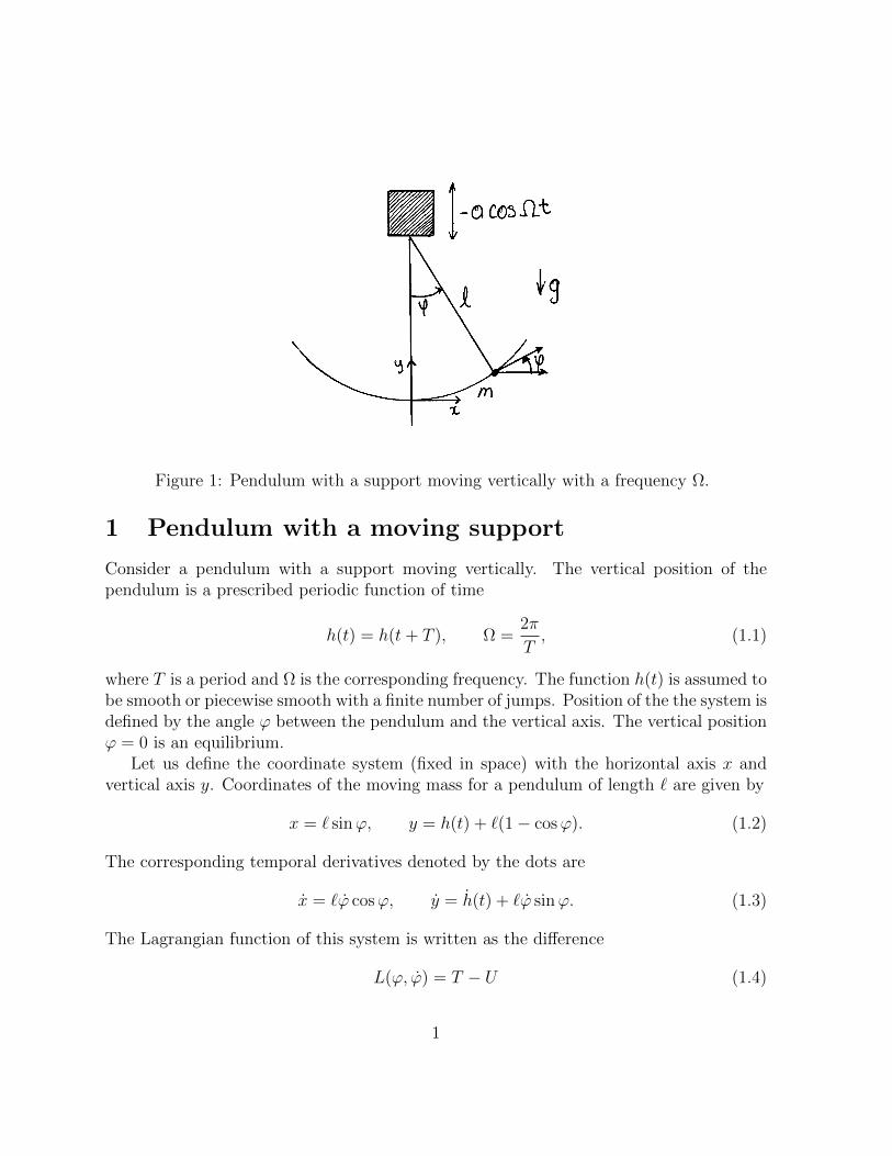
Figure 1: Pendulum with a support moving vertically with a frequency Ω.

1 Pendulum with a moving support

Consider a pendulum with a support moving vertically. The vertical position of thependulum is a prescribed periodic function of time

h(t) = h(t+ T ), Ω =2π

T, (1.1)

where T is a period and Ω is the corresponding frequency. The function h(t) is assumed tobe smooth or piecewise smooth with a finite number of jumps. Position of the the system isdefined by the angle ϕ between the pendulum and the vertical axis. The vertical positionϕ = 0 is an equilibrium.

Let us define the coordinate system (fixed in space) with the horizontal axis x andvertical axis y. Coordinates of the moving mass for a pendulum of length ` are given by

x = ` sinϕ, y = h(t) + `(1− cosϕ). (1.2)

The corresponding temporal derivatives denoted by the dots are

x = `ϕ cosϕ, y = h(t) + `ϕ sinϕ. (1.3)

The Lagrangian function of this system is written as the difference

L(ϕ, ϕ) = T − U (1.4)

1

of the kinetic and potential energies

T =m

2

(x2 + y2

), U = mgy, (1.5)

where g is the acceleration of gravity. Equations of motion are given by the Euler–Lagrange equation

d

dt

∂L

∂ϕ− ∂L

∂ϕ= 0, (1.6)

where d/dt is the material derivative taken along the system trajectory.Expressions (1.1)–(1.5) yield the final expression for the Lagrangian as

L = m`2

(ϕ2

2+hϕ

`sinϕ+

g

`cosϕ

), (1.7)

where we omitted all terms that do not depend on ϕ or ϕ and, therefore, will not appearin the final equation (1.6). Using this function in the Euler–Lagrange equation (1.6) yields

d

dt

(ϕ+

h

`sinϕ

)−

(hϕ

`cosϕ− g

`sinϕ

)= 0, (1.8)

where we dropped the common pre-factor m`2. Taking the material derivative, we derivethe final equation of motion in the form

ϕ+g

`

(1 +

h

g

)sinϕ = 0. (1.9)

This equation has a periodic coefficient h(t), which will lead to the phenomenon of para-metric resonance.

It is convenient to introduce and extra dependent variable ψ = ϕ and reduce thesystem to the system of first-order differential equations

y = g(y, t), (1.10)

where the vector y and the function g(y, t) are defined as

y =

(ϕ

ψ

), g(y, t) =

(ψ

−g`

(1 + h

g

)sinϕ

). (1.11)

This system has an equilibrium ϕ = ψ = 0 corresponding to the vertical position of thependulum.

2

2 Poincare map

Motivated by the example in the previous section, we consider a general system of theform

y = g(y, t), (2.1)

where y ∈ Rn and the right-hand side is a periodic function of time,

g(y, t) = g(y, t+ T ), (2.2)

with period T . Additionally, we assume that the system has an equilibrium (fixed-point)solution

y(t) ≡ y∗, (2.3)

which implies thatg(y∗, t) = 0 (2.4)

for all t ∈ R. This systems appear in various applications, where the periodic time-dependence may be caused by oscillations. For example, one may think of stability ofstructures under the action of waves, e.g., earthquakes or sea storms.

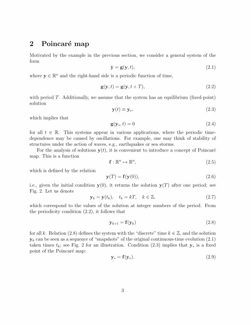
For the analysis of solutions y(t), it is convenient to introduce a concept of Poincaremap. This is a function

f : Rn 7→ Rn, (2.5)

which is defined by the relationy(T ) = f(y(0)), (2.6)

i.e., given the initial condition y(0), it returns the solution y(T ) after one period; seeFig. 2. Let us denote

yk = y(tk), tk = kT, k ∈ Z, (2.7)

which correspond to the values of the solution at integer numbers of the period. Fromthe periodicity condition (2.2), it follows that

yk+1 = f(yk) (2.8)

for all k. Relation (2.8) defines the system with the “discrete” time k ∈ Z, and the solutionyk can be seen as a sequence of “snapshots” of the original continuous-time evolution (2.1)taken times tk; see Fig. 2 for an illustration. Condition (2.3) implies that y∗ is a fixedpoint of the Poincare map:

y∗ = f(y∗). (2.9)

3

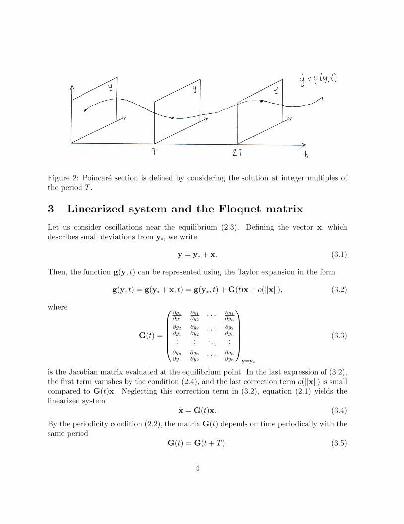
Figure 2: Poincare section is defined by considering the solution at integer multiples ofthe period T .

3 Linearized system and the Floquet matrix

Let us consider oscillations near the equilibrium (2.3). Defining the vector x, whichdescribes small deviations from y∗, we write

y = y∗ + x. (3.1)

Then, the function g(y, t) can be represented using the Taylor expansion in the form

g(y, t) = g(y∗ + x, t) = g(y∗, t) + G(t)x + o(‖x‖), (3.2)

where

G(t) =

∂g1∂y1

∂g1∂y2

· · · ∂g1∂yn

∂g2∂y1

∂g2∂y2

· · · ∂g2∂yn

......

. . ....

∂gn∂y1

∂gn∂y2

· · · ∂gn∂yn

y=y∗

(3.3)

is the Jacobian matrix evaluated at the equilibrium point. In the last expression of (3.2),the first term vanishes by the condition (2.4), and the last correction term o(‖x‖) is smallcompared to G(t)x. Neglecting this correction term in (3.2), equation (2.1) yields thelinearized system

x = G(t)x. (3.4)

By the periodicity condition (2.2), the matrix G(t) depends on time periodically with thesame period

G(t) = G(t+ T ). (3.5)

4

As an example, let us consider the system (1.11) with the equilibrium y∗ = 0. The matrixof the linearized system is easily derived as

G(t) =

(0 1

−g`

(1 + h

g

)0

). (3.6)

Similarly, one can linearize the discrete-time system (2.8). For this purpose, we definethe small deviation vectors xk from the fixed point as

yk = y∗ + xk. (3.7)

Using the Taylor expansion, the Poincare map is written as

f(yk) = f(y∗ + xk) = f(y∗) + Fxk + o(‖xk‖) = y∗ + Fxk + o(‖xk‖), (3.8)

where

F =

∂f1∂y1

∂f1∂y2

· · · ∂f1∂yn

∂f2∂y1

∂f2∂y2

· · · ∂f2∂yn

......

. . ....

∂fn∂y1

∂fn∂y2

· · · ∂fn∂yn

y=y∗

(3.9)

is the Jacobian matrix of f(y) evaluated at the fixed point. The matrix F does not dependon time and is called the Floquet matrix. Substituting yk+1 = y∗ + xk+1 and (3.8) into(2.8) and neglecting the nonlinear higher-order term o(‖xk‖), we obtain the linearizeddiscrete-time system in the form

xk+1 = Fxk. (3.10)

The relation between the continuous and discrete time variables (2.7) induces analo-gous relation for the linearized variables

xk = x(tk), tk = kT, k ∈ Z. (3.11)

This relation suggests a practical method for computing the Floquet matrix F as follows.Let us consider the Cauchy problem

X = G(t)X, X(0) = I (3.12)

for the n×n matrix function X(t), which is called the fundamental solution. Here, everycolumn of X(t) is a solution of the linearized system (3.4) for initial conditions equal tothe corresponding column of the identity matrix

I =

1 0 · · · 0

0 1 · · · 0...

.... . .

...

0 0 · · · 1

. (3.13)

5

One can see thatx(t) = X(t)x0 (3.14)

is a solution of the linearized system (3.4) for initial condition x(0) = x0. This yields

x1 = x(T ) = X(T )x0. (3.15)

Comparing this relation with (3.10) for k = 0, we obtain the Floquet matrix as

F = X(T ). (3.16)

This means that the Floquet matrix can be found by integrating the linearized system inone period.

4 Linear discrete-time dynamical system

In this section, we describe a general solution of the system

xk+1 = Fxk. (4.1)

For this purpose, let us consider the eigenvalue problem

Fu = ρu, (4.2)

where ρ ∈ C is an eigenvalue and u ∈ Cn is a corresponding eigenvector. Both ρ and umay take complex values. Each pair ρ and u defines an explicit solution

xk = ρku, (4.3)

which explains why eigenvalues of the Floquet matrix are also called the multipliers.When the multiplier ρ is real, the eigenvector u can also be taken real, which yields a realsolution (4.3). When ρ = |ρ|eiϕ is a complex number, we can construct real solutions bytaking real and imaginary parts of (4.3). This yields two different solutions

xk = |ρ|k [Re u cos(kϕ)− Im u sin(kϕ)] (4.4)

andxk = |ρ|k [Re u sin(kϕ) + Im u cos(kϕ)] . (4.5)

Exactly the same pair of solution is obtained for the complex conjugate eigenvalue ρ andeigenvector u. Thus the two solutions (4.4) and (4.5) are associated with the complexconjugate pair ρ and ρ.

Writing equation (4.2) as(F− ρI)u = 0, (4.6)

6

we conclude that the non-trivial solution u exists if and only if

det(F− ρI) = 0. (4.7)

This is the so-called characteristic equation. The left-hand side of this equation is apolynomial of degree n, which has n complex roots ρ1, . . . , ρn. In the case, when all theroots are simple (distinct), there are n corresponding eigenvector u1, . . . ,un, which arelinearly independent. Taking the linear combination of solutions (4.3) for all multipliers,we obtain a general solution

xk =n∑j=1

cjρkjuj, (4.8)

where cj are arbitrary coefficients. These coefficients are determined uniquely by theinitial condition

x0 =n∑j=1

cjuj, (4.9)

because the vectors u1, . . . ,un form a basis. This solution can be written in the real formby using expressions (4.4) and (4.5) instead of (4.3) for each complex conjugate pair ofmultipliers.

Example 1. Let is consider the matrix

F =

(2 11 2

). (4.10)

Characteristic equation (4.7) for this matrix takes the form

ρ2 − 4ρ+ 3 = 0 (4.11)

and yields two multipliersρ1 = 1, ρ2 = 3. (4.12)

The corresponding eigenvectors are found by solving the system (4.6) for each multiplieras

u1 =

(1−1

), u2 =

(11

). (4.13)

The general solution (4.8) is written in the form

xk = c1

(1−1

)+ c23

k

(11

)(4.14)

with arbitrary real coefficients c1 and c2.

7

Example 2. Let is consider the matrix

F =

(0 1−1 0

). (4.15)

Characteristic equation (4.7) for this matrix takes the form

ρ2 + 1 = 0 (4.16)

and yields two complex conjugate multipliers

ρ1 = i = eiπ/2, ρ2 = −i = e−iπ/2. (4.17)

The corresponding eigenvectors are found by solving the system (4.6) as

u1 =

(1i

), u2 =

(1−i

). (4.18)

The general solution (4.8) is written in the complex form

xk = c1ik

(1i

)+ c2(−i)k

(1−i

)(4.19)

with the complex coefficients c1 and c2. In order to obtain a real solution, one can takec1 = (a + ib)/2 and c2 = (a − ib)/2 with real numbers a and b. Then, expression (4.19)takes the form

xk = a

[(10

)cos

kπ

2−(

01

)sin

kπ

2

]+ b

[(10

)sin

kπ

2+

(01

)cos

kπ

2

]. (4.20)

The two solutions multiplied by a and b in this expression are exactly the two real solutions(4.4) and (4.5).

Example 3. Let is consider the matrix

F =

(3 1−1 1

). (4.21)

Characteristic equation (4.7) for this matrix takes the form

ρ2 − 4ρ+ 4 = 0 (4.22)

and yields two coincident rootsρ1 = ρ2 = 2. (4.23)

From the system (4.6) one obtains a single eigenvector

u =

(1−1

). (4.24)

In this case the general solution cannot be constructed in the form (4.8), because theeigenvectors do not form a basis. This example shows that the general solution is morecomplicated, when some of the eigenvalues are multiple.

8

5 Multiple eigenvalues and Jordan chains

Let us consider now the general case, when the eigenvalue ρ is not simple, i.e., it appearsma > 1 times as the root of the characteristic equation (4.7). The number ma is calledthe algebraic multiplicity (or simply the multiplicity) of the eigenvalue. Recall that theeigenvalue is called simple if ma = 1.

The number mg of linear independent eigenvectors corresponding to ρ is called itsgeometric multiplicity. From the linear algebra, we know that

1 ≤ mg ≤ ma. (5.1)

In the case mg = ma > 1, the eigenvalue ρ is called semi-simple: it is multiple, but has thesame number of linearly independent eigenvectors as the number of roots of characteristicequation. If all roots are simple or semi-simple, one can still write the general solution inthe form (4.8), because it is possible to form a basis with eigenvectors.

The solution becomes more complicated if mg < ma. In this case extra solutionsmust be determined. The linearly independent vectors u1, . . . ,u` form a Jordan chaincorresponding to ρ if they satisfy the system of equations

Fu1 = ρu1 (5.2)

Fu2 = ρu2 + u1 (5.3)...

Fu` = ρu` + u`−1, (5.4)

whileFu`+1 6= ρu`+1 + u` (5.5)

for any vector u`+1. Here u1 is the eigenvector and the other vectors u2, . . . ,u` are calledassociated vectors (or generalized eigenvectors). Note that these vectors are real for thereal ρ and complex for the complex ρ. Let us define a single n × ` matrix U with theJordan chains vectors takes as columns:

U = [u1 u2 · · · u`]. (5.6)

Then the chain (5.2)–(5.4) can be written as a single relatoin

FU = UJ, (5.7)

where

J =

ρ 1

ρ. . .. . . 1

ρ

(5.8)

9

is the m×m matrix called the Jordan block (it has the eigenvalue ρ on the main diagonal,unity on the upper diagonal and zeros otherwise).

Proposition 1. If u1, . . . ,u` are the Jordan chain vectors, then the following ` expressions

xk = ρku1, (5.9)

xk = ρku2 + kρk−1u1, (5.10)

...

xk = ρku` + kρk−1u`−1 + · · ·+ k!

`!(k − `)!ρk−`u1 (5.11)

are solutions of the system (4.1).

This statement can be verified by the direct substitution. For example, for the secondexpression, we have

Fxk = F(ρku2 +kρk−1u1) = ρk(ρu2 +u1)+kρku1 = ρk+1u2 +(k+1)ρku1 = xk+1, (5.12)

where we used the equations (5.2) and (5.3). Note that, for k = 0, expressions of Propo-sition 1 become

x0 = u1, (5.13)

x0 = u2, (5.14)

...

x0 = u`, (5.15)

which means that these ` solutions are linearly independent. We showed that a Jordanchain of length ` defines ` linearly independent solutions, which all stay in the linearsubspace spanned by the vectors of the Jordan chain.

The well-known result of linear algebra is the Jordan normal form theorem. It saysthat any matrix can be reduced to the Jordan canonical form by a non-singular complexmatrix C, i.e.,

C−1FC =

J1

. . .

JA

, (5.16)

where the right-hand side is a block-diagonal matrix and J1, . . . ,JA are Jordan blocks thatcontain all eigenvalues of the matrix F. Splitting the columns of matrix C = [U1 · · · UA],one can see that each set of vectors Ua is the Joran chain with the Jordan block Ja, wherea = 1, . . . , A; see Eq. 5.7.

10

Theorem 1. Consider a basis provided by the Jordan form theorem and constructed withthe vectors of Jordan chains for all eigenvalues. Then, the general solution of system(4.1) is obtained by taking a linear combination of solutions described in Proposition 1 forall eigenvalues and corresponding Jordan chains.

Note that the geometric multiplicity mg of the eigenvalue defines a number differentJordan chains (Jordan blocks). Let `1, . . . , `mg are lengths of such Jordan chains (sizes ofJordan blocks). Then, the algebraic multiplicity is equal to the total number of vectorsin these chains: ma = `1 + · · ·+ `mg .

Example 4. We have shown in Example 3 that the matrix (4.21) has a multipleeigenvalue ρ = 2 of algebraic multiplicity ma = 2 and geometric multiplicity mg = 1.This means that there must be a Jordan chain, which consists of the eigenvector u1 andthe associated vector u2. By solving equations (5.2) and (5.3), we obtain

u1 =

(1−1

), u2 =

(10

). (5.17)

The general solution is obtained as a linear combination of solutions (5.9) and (5.10):

xk = (c12k + c2k2k−1)

(1−1

)+ c22

k

(10

). (5.18)

6 Stability theory

We now can formulate the concepts of Lyapunov stability for equilibrium solutions incontinuous- and discrete-time systems.

Definition 1. The equilibrium solution y(t) ≡ y∗ of system (2.1) is called

• stable if for any ε > 0 there exists δ > 0, such that solutions remain ε-close to theequilibrium, i.e.,

‖y(t)− y∗‖ < ε, (6.1)

for all times t ≥ 0 and initial conditions satisfying

‖y(0)− y∗‖ < δ. (6.2)

• asymptotically stable if for any ε > 0 there exists δ > 0, such that

‖y(t)− y∗‖ < ε for t ≥ 0 (6.3)

andlimt→+∞

y(t)− y∗ (6.4)

for all initial conditions satisfying (6.2).

11

The concept of stability is formulated similarly for discrete-time systems.

Definition 2. The equilibrium solution yk ≡ y∗ of system (2.8) is called

• stable if for any ε > 0 there exists δ > 0, such that solutions remain ε-close to theequilibrium, i.e.,

‖yk − y∗‖ < ε, (6.5)

for all k ≥ 0 and initial conditions satisfying

‖y0 − y∗‖ < δ. (6.6)

• asymptotically stable if for any ε > 0 there exists δ > 0, such that

‖yk − y∗‖ < ε for k ≥ 0 (6.7)

andlim

k→+∞yk = y∗ (6.8)

for all initial conditions satisfying (6.6).

In our case, these two definitions are in fact equivalent:

Proposition 2. The equilibrium solution y(t) ≡ y∗ of system (2.1) is (asymptotically)stable if and only if the equilibrium solution yk ≡ y∗ is (asymptotically) stable for thePoincare map (2.8).

This proposition follows from the continuous dependence of solutions of ordinary differ-ential equations on initial conditions. Now, let us formulate the stability criteria. Thefirst result provides the complete stability description in the case of linear systems.

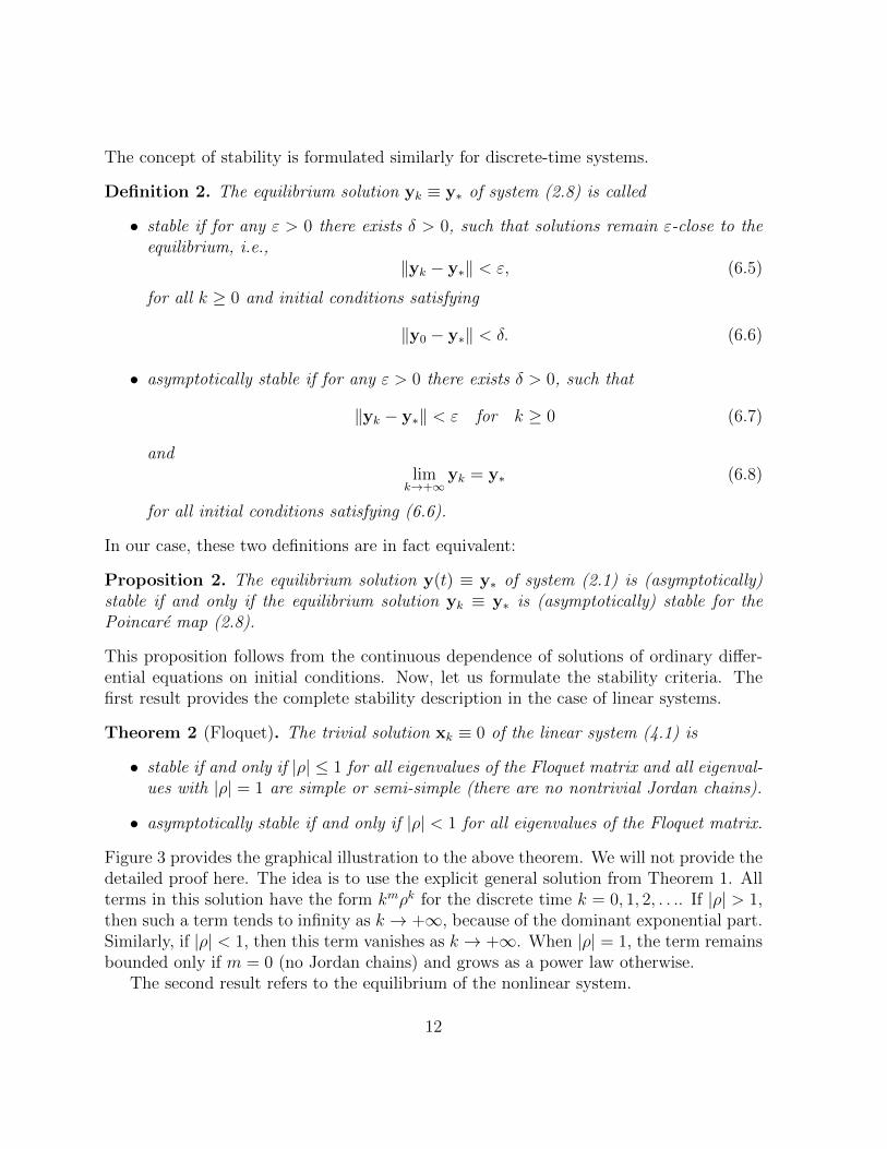
Theorem 2 (Floquet). The trivial solution xk ≡ 0 of the linear system (4.1) is

• stable if and only if |ρ| ≤ 1 for all eigenvalues of the Floquet matrix and all eigenval-ues with |ρ| = 1 are simple or semi-simple (there are no nontrivial Jordan chains).

• asymptotically stable if and only if |ρ| < 1 for all eigenvalues of the Floquet matrix.

Figure 3 provides the graphical illustration to the above theorem. We will not provide thedetailed proof here. The idea is to use the explicit general solution from Theorem 1. Allterms in this solution have the form kmρk for the discrete time k = 0, 1, 2, . . .. If |ρ| > 1,then such a term tends to infinity as k → +∞, because of the dominant exponential part.Similarly, if |ρ| < 1, then this term vanishes as k → +∞. When |ρ| = 1, the term remainsbounded only if m = 0 (no Jordan chains) and grows as a power law otherwise.

The second result refers to the equilibrium of the nonlinear system.

12

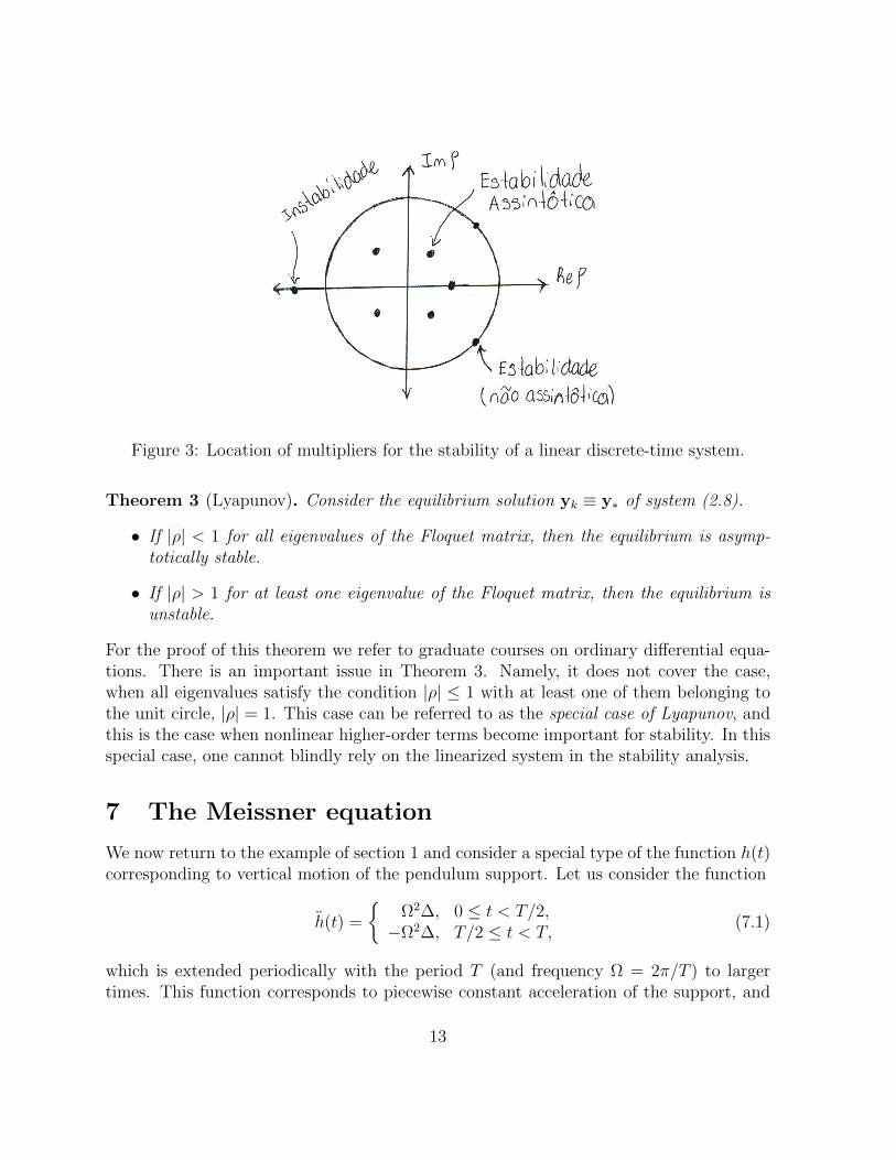
Figure 3: Location of multipliers for the stability of a linear discrete-time system.

Theorem 3 (Lyapunov). Consider the equilibrium solution yk ≡ y∗ of system (2.8).

• If |ρ| < 1 for all eigenvalues of the Floquet matrix, then the equilibrium is asymp-totically stable.

• If |ρ| > 1 for at least one eigenvalue of the Floquet matrix, then the equilibrium isunstable.

For the proof of this theorem we refer to graduate courses on ordinary differential equa-tions. There is an important issue in Theorem 3. Namely, it does not cover the case,when all eigenvalues satisfy the condition |ρ| ≤ 1 with at least one of them belonging tothe unit circle, |ρ| = 1. This case can be referred to as the special case of Lyapunov, andthis is the case when nonlinear higher-order terms become important for stability. In thisspecial case, one cannot blindly rely on the linearized system in the stability analysis.

7 The Meissner equation

We now return to the example of section 1 and consider a special type of the function h(t)corresponding to vertical motion of the pendulum support. Let us consider the function

h(t) =

Ω2∆, 0 ≤ t < T/2,−Ω2∆, T/2 ≤ t < T,

(7.1)

which is extended periodically with the period T (and frequency Ω = 2π/T ) to largertimes. This function corresponds to piecewise constant acceleration of the support, and

13

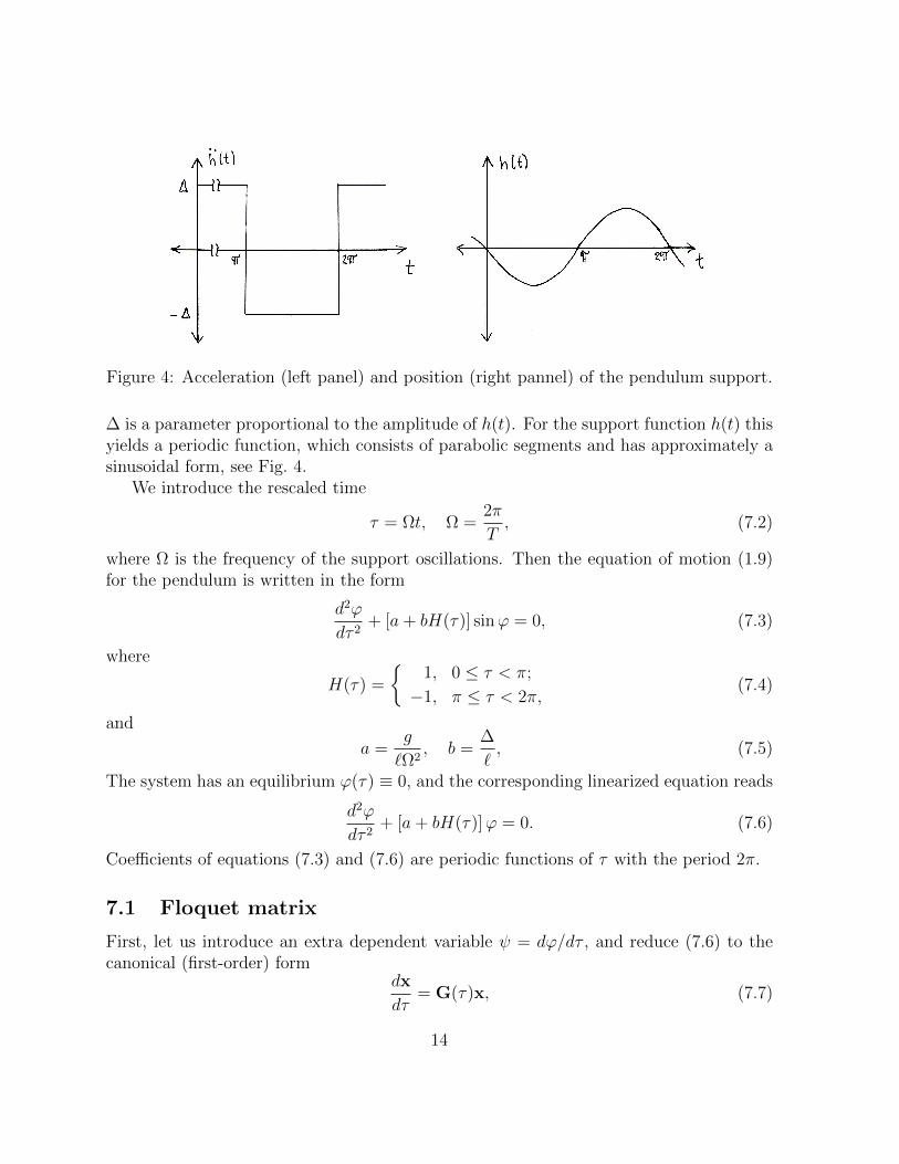
Figure 4: Acceleration (left panel) and position (right pannel) of the pendulum support.

∆ is a parameter proportional to the amplitude of h(t). For the support function h(t) thisyields a periodic function, which consists of parabolic segments and has approximately asinusoidal form, see Fig. 4.

We introduce the rescaled time

τ = Ωt, Ω =2π

T, (7.2)

where Ω is the frequency of the support oscillations. Then the equation of motion (1.9)for the pendulum is written in the form

d2ϕ

dτ 2+ [a+ bH(τ)] sinϕ = 0, (7.3)

where

H(τ) =

1, 0 ≤ τ < π;

−1, π ≤ τ < 2π,(7.4)

and

a =g

`Ω2, b =

∆

`, (7.5)

The system has an equilibrium ϕ(τ) ≡ 0, and the corresponding linearized equation reads

d2ϕ

dτ 2+ [a+ bH(τ)]ϕ = 0. (7.6)

Coefficients of equations (7.3) and (7.6) are periodic functions of τ with the period 2π.

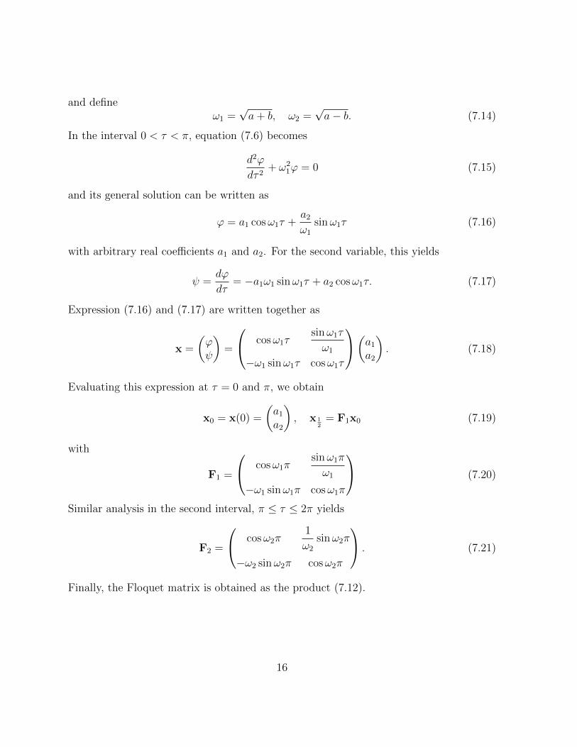
7.1 Floquet matrix

First, let us introduce an extra dependent variable ψ = dϕ/dτ , and reduce (7.6) to thecanonical (first-order) form

dx

dτ= G(τ)x, (7.7)

14

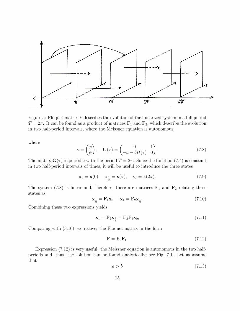
Figure 5: Floquet matrix F describes the evolution of the linearized system in a full periodT = 2π. It can be found as a product of matrices F1 and F2, which describe the evolutionin two half-period intervals, where the Meissner equation is autonomous.

where

x =

(ϕψ

), G(τ) =

(0 1

−a− bH(τ) 0

). (7.8)

The matrix G(τ) is periodic with the period T = 2π. Since the function (7.4) is constantin two half-period intervals of times, it will be useful to introduce the three states

x0 = x(0), x 12

= x(π), x1 = x(2π). (7.9)

The system (7.8) is linear and, therefore, there are matrices F1 and F2 relating thesestates as

x 12

= F1x0, x1 = F2x 12. (7.10)

Combining these two expressions yields

x1 = F2x 12

= F2F1x0, (7.11)

Comparing with (3.10), we recover the Floquet matrix in the form

F = F2F1. (7.12)

Expression (7.12) is very useful: the Meissner equation is autonomous in the two half-periods and, thus, the solution can be found analytically; see Fig. 7.1. Let us assumethat

a > b (7.13)

15

and defineω1 =

√a+ b, ω2 =

√a− b. (7.14)

In the interval 0 < τ < π, equation (7.6) becomes

d2ϕ

dτ 2+ ω2

1ϕ = 0 (7.15)

and its general solution can be written as

ϕ = a1 cosω1τ +a2ω1

sinω1τ (7.16)

with arbitrary real coefficients a1 and a2. For the second variable, this yields

ψ =dϕ

dτ= −a1ω1 sinω1τ + a2 cosω1τ. (7.17)

Expression (7.16) and (7.17) are written together as

x =

(ϕψ

)=

cosω1τsinω1τ

ω1

−ω1 sinω1τ cosω1τ

(a1a2

). (7.18)

Evaluating this expression at τ = 0 and π, we obtain

x0 = x(0) =

(a1a2

), x 1

2= F1x0 (7.19)

with

F1 =

cosω1πsinω1π

ω1

−ω1 sinω1π cosω1π

(7.20)

Similar analysis in the second interval, π ≤ τ ≤ 2π yields

F2 =

cosω2π1

ω2

sinω2π

−ω2 sinω2π cosω2π

. (7.21)

Finally, the Floquet matrix is obtained as the product (7.12).

16

7.2 Stability conditions

It is easy to see thatdet F1 = 1, det F2 = 1. (7.22)

This means thatdet F = det (F2F1) = det F1 det F2 = 1. (7.23)

Recall that the determinant of the Floquet matrix equals to the product of its eigenvaluesρ1 and ρ2:

det F = ρ1ρ2. (7.24)

At the same time, the sum of the eigenvalues equals to the trance of the matrix:

tr F = ρ1 + ρ2. (7.25)

Also, if ρ1 is complex, we have ρ2 = ρ1.Hence, there are three possibilities:

(a) the eigenvalues are real and distinct with ρ2 = 1/ρ1. In this case |tr F| > 2. ByTheorem 2, the equilibrium of the linear system is unstable, because |ρ| > 1 for oneof the eigenvalues.

(b) the two distinct eigenvalues are complex conjugate with the unit absolute value:ρ1,2 = e±iα. In this case |tr F| < 2. By Theorem 2, the equilibrium of the linearsystem is stable.

(c) The intermediate case, when the eigenvalues are mulitple (double) with the valueρ1 = ρ2 = 1 or ρ1 = ρ2 = −1. In this case |tr F| = 2. Stability or instability dependson the Jordan structure of this double eigenvalue.

Summarizing, we have the following stability criteria

stability : tr F < 2, (7.26)

instability : tr F > 2, (7.27)

stability boundary : tr F = 2. (7.28)

The trace of the Floquet matrix is computed from the relations (7.12), (7.20) and (7.21)as

tr F = 2 cosω1π cosω2π −(ω1

ω2

+ω2

ω1

)sinω1π sinω2π. (7.29)

17

7.3 Stability diagram

Let us describe now the structure of instability regions in the parameter plane (a, b).These parameters are related to ω1 and ω2 by relations (7.14). Our analysis will be basedon the relation

tr F = 2

∣∣∣∣cosω1π cosω2π −(ω1

ω2

+ω2

ω1

)sinω1π sinω2π

∣∣∣∣ = 2, (7.30)

which according to (7.28) and (7.29) defines the boundary between stability and instabilitydomains. small amplitudes ∆ of the support oscillation correspond to small values of b,which implies ω1 ≈ ω2. In particular, for the case ∆ = 0 (pendulum with a fixed support),we have b = 0 and ω1 = ω2 =

√a. Then, expression (7.29) reduces to

tr F = 2 cos2(π√a)− 2 sin2

(π√a)

= 2 cos(2π√a). (7.31)

Thus, tr F ≤ 2 and, hence, the system is stable. This is expected because the pendulumwith a fixed support is stable. However, the boundary condition (7.30) is satisfied onlywhen 2

√a is integer. This yields a set of resonant points

(a, b) =

(n2

4, 0

), n = 1, 2, . . . (7.32)

These points mark the locations of possible instability regions, which may appear fornonzero but small values of b. Odd and even values of n correspond to different types ofdouble eigenvalues

odd n : ρ1 = ρ2 = −1; even n : ρ1 = ρ2 = 1. (7.33)

For example, let us consider the parameters

a =1

4+ε2

π2, b =

ε

π(7.34)

for small ε, in which case

ω1 =1

2+ε

π, ω2 =

1

2− ε

π. (7.35)

Computing the trace (7.29) yields

tr F = −2

(sin2 ε+

1/4 + ε2/π2

1/4− ε2/π2cos2 ε

). (7.36)

Since the pre-factor of cos2 ε is greater than unity, we have |tr F| > 2 for small positive εand, hence, the system is unstable.

18

The form of instability zones near the resonant points (7.32) can be found by asymp-totic methods or numerically. They have the form of “tongues” as illustrated in Fig. 6; thestability diagram is symmetric for positive and negative b. The form of instability zonesfor larger values of b is presented in Fig. 7. Note that the boundaries of each instabilityzone passing through a resonant point (7.32) is characterized by a negative (for odd n)or positive (for even n) double eigenvalue, as described in (7.33). Since the boundariesof the adjacent zones correspond to different double eigenvalues, they cannot intersect.However, boundaries of the same zone may have self-intersections. Figure 8 shows thechange of eigenvalues with increasing a and fixed small value of b.

8 Mathieu equation

Let us considers the support of the pendulum oscillating as

h(t) = −∆ cos Ωt. (8.1)

The change of variables (7.2) and parameters (7.5) yields the Mathieu equation

d2ϕ

dτ 2+ (a+ b cos τ)ϕ = 0. (8.2)

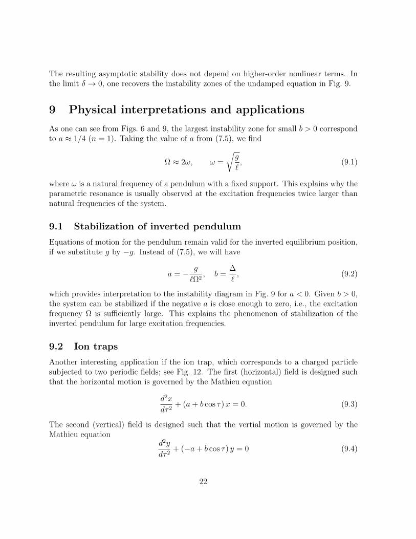
Analysis of this equation is similar to the case of the Meissner equation, except thatthe solution for the Floquet matrix cannot be found analytically. However, both systemscoincide for b = 0 and, therefore, the resonant points (7.32) are the same. These resonancepoints give rise to instability regions shown in Fig. 9. In this figure we also showed theinstability region for negative values of a.

Notice that the stability in (7.26) was not asymptotic, because both eigenvalues belongto the unit circle. Thus, this is the special case of Lyaunov, and one cannot say ifthe equilibrium is stable or not for the original nonlinear system. One of the ways tounderstand the stability properties for the nonlinear system is to add a small dissipativeterm into the equation of motion. For the linearized system the resulting damped Mathieuequation becomes

d2ϕ

dτ 2+ δ

dϕ

dτ+ (a+ b cos τ)ϕ = 0, (8.3)

where δ > 0 is a small damping coefficient. Stability analysis of this system, or analogoussystem for the damped Meissner equation, uses the same ideas, with the difference thatthe eigenvalues do not satisfy any more the relation ρ1ρ2 = 1. It turns out that theeigenvalues, which were on the unit circle for the undamped system, are shifted inside theunit circle, when small damping is added; see Fig. 10. As a result, the stability regionsincrease and become the regions of asymptotic stability with both eigenvalues |ρ| < 1when we add a damping term; see Fig. 11. Accordingly, the instability zones decrease.

19

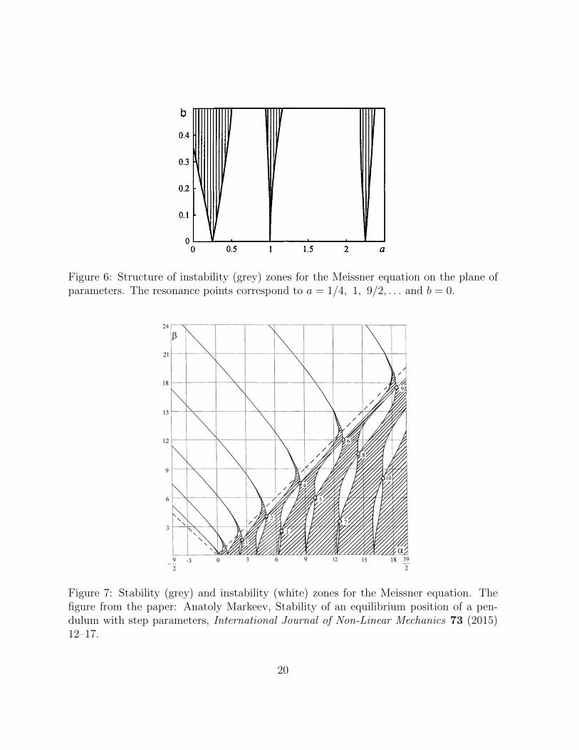
Figure 6: Structure of instability (grey) zones for the Meissner equation on the plane ofparameters. The resonance points correspond to a = 1/4, 1, 9/2, . . . and b = 0.

Figure 7: Stability (grey) and instability (white) zones for the Meissner equation. Thefigure from the paper: Anatoly Markeev, Stability of an equilibrium position of a pen-dulum with step parameters, International Journal of Non-Linear Mechanics 73 (2015)12–17.

20

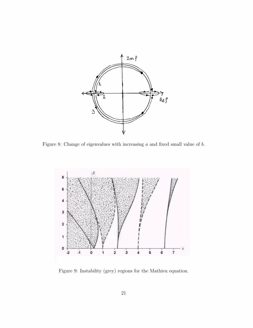
Figure 8: Change of eigenvalues with increasing a and fixed small value of b.

Figure 9: Instability (grey) regions for the Mathieu equation.

21

The resulting asymptotic stability does not depend on higher-order nonlinear terms. Inthe limit δ → 0, one recovers the instability zones of the undamped equation in Fig. 9.

9 Physical interpretations and applications

As one can see from Figs. 6 and 9, the largest instability zone for small b > 0 correspondto a ≈ 1/4 (n = 1). Taking the value of a from (7.5), we find

Ω ≈ 2ω, ω =

√g

`, (9.1)

where ω is a natural frequency of a pendulum with a fixed support. This explains why theparametric resonance is usually observed at the excitation frequencies twice larger thannatural frequencies of the system.

9.1 Stabilization of inverted pendulum

Equations of motion for the pendulum remain valid for the inverted equilibrium position,if we substitute g by −g. Instead of (7.5), we will have

a = − g

`Ω2, b =

∆

`, (9.2)

which provides interpretation to the instability diagram in Fig. 9 for a < 0. Given b > 0,the system can be stabilized if the negative a is close enough to zero, i.e., the excitationfrequency Ω is sufficiently large. This explains the phenomenon of stabilization of theinverted pendulum for large excitation frequencies.

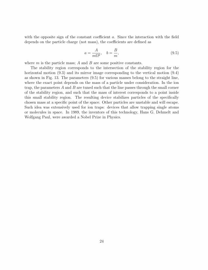
9.2 Ion traps

Another interesting application if the ion trap, which corresponds to a charged particlesubjected to two periodic fields; see Fig. 12. The first (horizontal) field is designed suchthat the horizontal motion is governed by the Mathieu equation

d2x

dτ 2+ (a+ b cos τ)x = 0. (9.3)

The second (vertical) field is designed such that the vertial motion is governed by theMathieu equation

d2y

dτ 2+ (−a+ b cos τ) y = 0 (9.4)

22

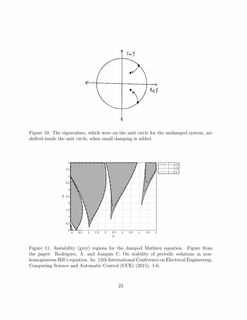
Figure 10: The eigenvalues, which were on the unit circle for the undamped system, areshifted inside the unit circle, when small damping is added.

Figure 11: Instability (grey) regions for the damped Mathieu equation. Figure fromthe paper: Rodriguez, A. and Joaquın C. On stability of periodic solutions in non-homogeneous Hill’s equation. In: 12th International Conference on Electrical Engineering,Computing Science and Automatic Control (CCE) (2015): 1-6.

23

with the opposite sign of the constant coefficient a. Since the interaction with the fielddepends on the particle charge (not mass), the coefficients are defined as

a =A

mΩ2, b =

B

m, (9.5)

where m is the particle mass; A and B are some positive constants.The stability region corresponds to the intersection of the stability region for the

horizontal motion (9.3) and its mirror image corresponding to the vertical motion (9.4)as shown in Fig. 13. The parameters (9.5) for various masses belong to the straight line,where the exact point depends on the mass of a particle under consideration. In the iontrap, the parameters A and B are tuned such that the line passes through the small cornerof the stability region, and such that the mass of interest corresponds to a point insidethis small stability region. The resulting device stabilizes particles of the specificallychosen mass at a specific point of the space. Other particles are unstable and will escape.Such idea was extensively used for ion traps: devices that allow trapping single atomsor molecules in space. In 1989, the inventors of this technology, Hans G. Dehmelt andWolfgang Paul, were awarded a Nobel Prize in Physics.

24

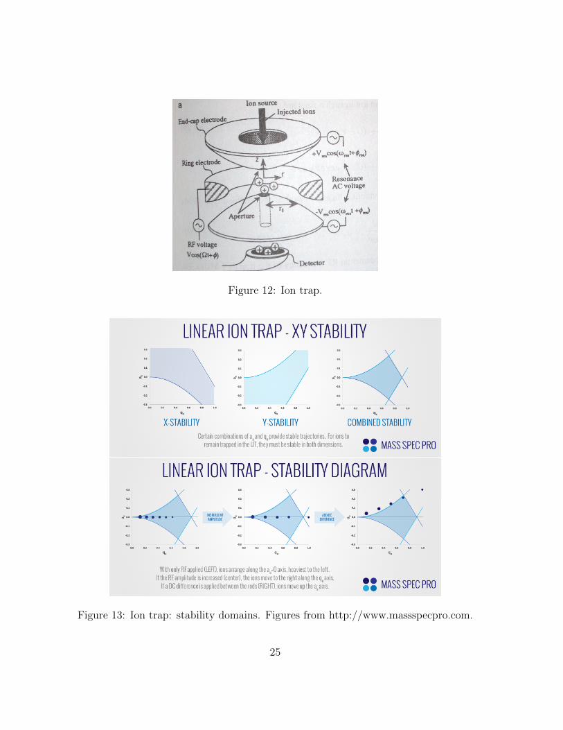
Figure 12: Ion trap.

Figure 13: Ion trap: stability domains. Figures from http://www.massspecpro.com.

25