Nils Lid Hjort1, Ian W. McKeague2, and Ingrid Van Keilegom3
University of Oslo, Columbia University, and KU Leuven
Abstract: This paper develops a hybrid likelihood (HL) method based on a compromise between
parametric and nonparametric likelihoods. Consider the setting of a parametric model for the
distribution of an observation Y with parameter θ. Suppose there is also an estimating function
m(·, µ) identifying another parameter µ via Em(Y, µ) = 0, at the outset defined independently of
the parametric model. To borrow strength from the parametric model while obtaining a degree of
robustness from the empirical likelihood method, we formulate inference about θ in terms of the
hybrid likelihood function Hn(θ) = Ln(θ)1−aRn(µ(θ))a. Here a ∈ [0, 1) represents the extent of the
compromise, Ln is the ordinary parametric likelihood for θ, Rn is the empirical likelihood function,
and µ is considered through the lens of the parametric model. We establish asymptotic normality
of the corresponding HL estimator and a version of the Wilks theorem. We also examine extensions
of these results under misspecification of the parametric model, and propose methods for selecting
the balance parameter a.
tion, Robust methods
Some personal reflections on Peter
We are all grateful to Peter for his deeply influential contributions to the field of statistics, in particular to
the areas of nonparametric smoothing, bootstrap, empirical likelihood (what this paper is about), functional
data, high-dimensional data, measurement errors, etc., many of which were major breakthroughs in the area.
His services to the profession were also exemplary and exceptional. It seems that he could simply not say
‘no’ to the many requests for recommendation letters, thesis reports, editorial duties, departmental reviews,
and various other requests for help, and as many of us have experienced, he handled all this with an amazing
speed, thoroughness and efficiency. We will also remember Peter as a very warm, gentle and humble person,
who was particularly supportive to young people.
Nils Lid Hjort: I have many and uniformly warm remembrances of Peter. We had met and talked a few
times at conferences, and then Peter invited me for a two-month stay in Canberra in 2000. This was both
1N.L. Hjort is supported via the Norwegian Research Council funded project FocuStat. 2I.W. McKeague is partially supported by NIH Grant R01GM095722. 3I. Van Keilegom is financially supported by the European Research Council (2016-2021, Horizon 2020, grant agreement No.
694409), and by IAP research network grant nr. P7/06 of the Belgian government (Belgian Science Policy).
2 NILS LID HJORT, IAN W. MCKEAGUE, and INGRID VAN KEILEGOM
enjoyable, friendly and fruitful. I remember fondly not only technical discussions and the free-flowing of ideas
on blackboards (and since Peter could think twice as fast as anyone else, that somehow improved my own
arguing and thinking speed, or so I’d like to think), but also the positive, widely international, upbeat, but
unstressed working atmosphere. Among the pluses for my Down Under adventures were not merely meeting
kangaroos in the wild while jogging and singing Schnittke, but teaming up with fellow visitors for several
good projects, in particular with Gerda Claeskens; another sign of Peter’s deep role in building partnerships
and teams around him, by his sheer presence.
Then Peter and Jeannie visited us in Oslo for a six-week period in the autumn of 2003. For their first day
there, at least Jeannie was delighted that I had put on my Peter Hall t-shirt and that I gave him a Hall of
Fame wristwatch. For these Oslo weeks he was therefore elaboratedly introduced at seminars and meetings
as Peter Hall of Fame; everyone understood that all other Peter Halls were considerably less famous. A
couple of project ideas we developed together, in the middle of Peter’s dozens and dozens of other ongoing
real-time projects, are still in my drawers and files, patiently awaiting completion. Very few people can be
as quietly and undramatically supremely efficient and productive as Peter. Luckily most of us others don’t
really have to, as long as we are doing decently well a decent proportion of the time. But once in a while, in
my working life, when deadlines are approaching and I’ve lagged far behind, I put on my Peter Hall t-shirt,
and think of him. It tends to work.
Ingrid Van Keilegom: I first met Peter in 1995 during one of Peter’s many visits to Louvain-la-Neuve
(LLN). At that time I was still a graduate student at Hasselt University. Two years later, in 1997, Peter
obtained an honorary doctorate from the Institute of Statistics in LLN (at the occasion of the fifth anniversary
of the Institute), during which I discovered that Peter was not only a giant in his field but also a very human,
modest and kind person. Figure 1(a) shows Peter at his acceptance speech. Later, in 2002, soon after I
started working as a young faculty member in LLN, Peter invited me to Canberra for six weeks, a visit of
which I have extremely positive memories. I am very grateful to Peter for having given me the opportunity
to work with him there. During this visit Peter and I started working on two papers, and although Peter
HYBRID EMPIRICAL LIKELIHOOD 3
(a) (b)
Figure 1: (a) Peter at the occasion of his honorary doctorate at the Institute of Statistics in Louvain-la-Neuve in 1997; (b) Peter and Ingrid Van Keilegom in Tidbinbilla Nature Reserve near Canberra in 2002 (picture taking by Jeannie Hall).
was very busy with many other things, it was difficult to stay on top of all new ideas and material that he
was suggesting and adding to the papers, day after day. At some point during this visit Peter left Canberra
for a 10-day visit to London, and I (naively) thought I could spend more time on broadening my knowledge
on the two topics Peter had introduced to me. However, the next morning I received a fax of 20 pages of
hand-written notes, containing a difficult proof that Peter had found during the flight to London. It took
me the full next 10 days to unraffle all the details of the proof! Although Peter was very focused and busy
with his work, he often took his visitors on a trip during the weekends. I enjoyed very much the trip to the
Tidbinbilla Nature Reserve near Canberra, together with him and his wife Jeannie. A picture taken in this
park by Jeannie is seen in Figure 1(b).
After the visit to Canberra, Peter and I continued working on other projects, and in around 2004 Peter
visited LLN for several weeks. I picked him up in the morning from the airport in Brussels. He came straight
from Canberra and had been more or less 30 hours underway. I supposed without asking that he would like
to go to the hotel to take a rest. But when we were approaching the hotel, Peter insisted that I would drive
immediately to the Institute in order to start working straight away. He spent the whole day at the Institute
discussing with people and working in his office, before going finally to his hotel! I always wondered where
4 NILS LID HJORT, IAN W. MCKEAGUE, and INGRID VAN KEILEGOM
he found the energy, the motivation and the strength to do this. He will be remembered by many of us as
an extremely hard working person, and as an example to all of us.
HYBRID EMPIRICAL LIKELIHOOD 5
1 Introduction
For modelling data there are usually many options, ranging from purely parametric, semiparametric, to fully
nonparametric. There are also numerous ways in which to combine parametrics with nonparametrics, say
estimating a model density by a combination of a parametric fit with a nonparametric estimator, or by taking
a weighted average of parametric and nonparametric quantile estimators. This article concerns a proposal
for a bridge between a given parametric model and a nonparametric likelihood-ratio method. We construct
a hybrid likelihood function, based on (i) the usual likelihood function for the parametric model, say Ln(θ),
with n referring to sample size, as usual; and (ii) the empirical likelihood function for a given set of control
parameters, say Rn(µ), where the µ parameters in question are “pushed through” the parametric model,
leading to Rn(µ(θ)), say. Our hybrid likelihood Hn(θ), defined in (2) below, will be used for estimating
the parameter vector of the working model; we term the θhl in question the maximum hybrid likelihood
estimator. This in turn leads to estimates of other quantities of interest. If ψ is such a focus parameter,
expressed via the working model as ψ = ψ(θ), then it will be estimated using ψhl = ψ(θhl).
If the working parametric model is correct, these hybrid estimators will lose a certain amount in terms of
efficiency, when compared to the usual maximum likelihood estimator. We shall demonstrate, however, that
the efficiency loss under ideal model conditions is typically a small one, and that the hybrid estimators often
will outperform the maximum likelihood when the working model is not correct. Thus the hybrid likelihood
will be seen to offer parametric robustness, or protection against model misspecification, by borrowing
strength from the empirical likelihood, via the selected control parameters.
Though our construction and methods can be lifted to e.g. regression models, see Section S.5 in the
supplementary material, it is practical to start with the simpler i.i.d. framework, both for conveying the
basic ideas and for developing theory. Thus let Y1, ..., Yn be i.i.d. observations, stemming from some unknown
density f . We wish to fit the data to some parametric family, say fθ(y) = f(y, θ), with θ = (θ1, . . . , θp) t ∈ Θ,
where Θ is an open subset of Rp . The purpose of fitting the data to the model is typically to make inference
about certain quantities ψ = ψ(f), termed focus parameters, but without necessarily trusting the model
6 NILS LID HJORT, IAN W. MCKEAGUE, and INGRID VAN KEILEGOM
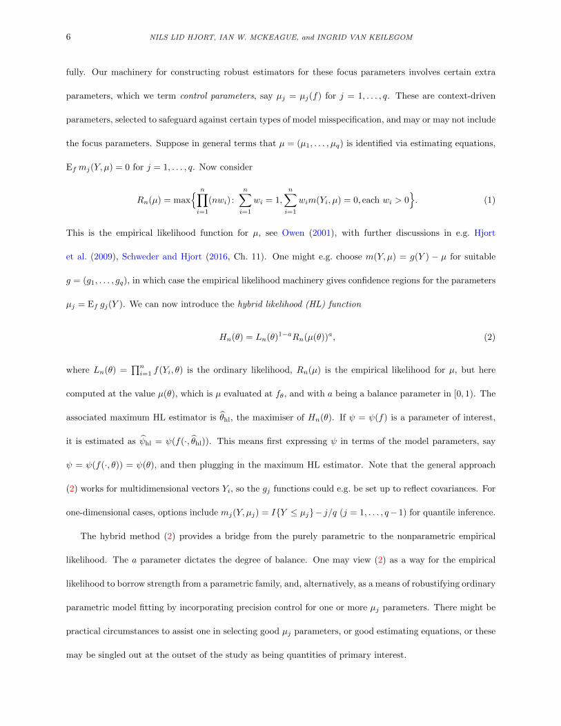
fully. Our machinery for constructing robust estimators for these focus parameters involves certain extra
parameters, which we term control parameters, say µj = µj(f) for j = 1, . . . , q. These are context-driven
parameters, selected to safeguard against certain types of model misspecification, and may or may not include
the focus parameters. Suppose in general terms that µ = (µ1, . . . , µq) is identified via estimating equations,
Ef mj(Y, µ) = 0 for j = 1, . . . , q. Now consider
Rn(µ) = max { n∏ i=1
(nwi) :
wim(Yi, µ) = 0, each wi > 0 } . (1)
This is the empirical likelihood function for µ, see Owen (2001), with further discussions in e.g. Hjort
et al. (2009), Schweder and Hjort (2016, Ch. 11). One might e.g. choose m(Y, µ) = g(Y ) − µ for suitable
g = (g1, . . . , gq), in which case the empirical likelihood machinery gives confidence regions for the parameters
µj = Ef gj(Y ). We can now introduce the hybrid likelihood (HL) function
Hn(θ) = Ln(θ)1−aRn(µ(θ))a, (2)
where Ln(θ) = ∏n i=1 f(Yi, θ) is the ordinary likelihood, Rn(µ) is the empirical likelihood for µ, but here
computed at the value µ(θ), which is µ evaluated at fθ, and with a being a balance parameter in [0, 1). The
associated maximum HL estimator is θhl, the maximiser of Hn(θ). If ψ = ψ(f) is a parameter of interest,
it is estimated as ψhl = ψ(f(·, θhl)). This means first expressing ψ in terms of the model parameters, say
ψ = ψ(f(·, θ)) = ψ(θ), and then plugging in the maximum HL estimator. Note that the general approach
(2) works for multidimensional vectors Yi, so the gj functions could e.g. be set up to reflect covariances. For
one-dimensional cases, options include mj(Y, µj) = I{Y ≤ µj}− j/q (j = 1, . . . , q−1) for quantile inference.
The hybrid method (2) provides a bridge from the purely parametric to the nonparametric empirical
likelihood. The a parameter dictates the degree of balance. One may view (2) as a way for the empirical
likelihood to borrow strength from a parametric family, and, alternatively, as a means of robustifying ordinary
parametric model fitting by incorporating precision control for one or more µj parameters. There might be
practical circumstances to assist one in selecting good µj parameters, or good estimating equations, or these
may be singled out at the outset of the study as being quantities of primary interest.
HYBRID EMPIRICAL LIKELIHOOD 7
Example 1. Let fθ be the normal density with parameters (ξ, σ2), and use mj(y, µj) = I{y ≤ µj}− j/4 for
j = 1, 2, 3. Then (1.1), with the ensuing µj(ξ, σ) = ξ + σΦ−1(j/4) for j = 1, 2, 3, may be seen as estimating
the normal parameters in a way which modifies the parametric ML method by taking into account the wish
to have good model fit for the three quartiles. Alternatively, it may be viewed as a way of making inference
for the three quartiles, borrowing strength from the normal family in order to hopefully do better than
simply using the three empirical quartiles.
Example 2. Let fθ be the Beta family with parameters (b, c), where ML estimates match moments for
log Y and log(1− Y ). Add to these the functions mj(y, µj) = yj −µj for j = 1, 2. Again, this is Beta fitting
with modification for getting the mean and variance about right, or moment estimation borrowing strength
from the Beta family.
Example 3. Take your favourite parametric family f(y, θ), and for an appropriate data set specify an
interval or region A that actually matters. Then use m(y, p) = I{y ∈ A}−p as ‘control equation’ above, with
p = P{Y ∈ A} = ∫ A f(y, θ) dy. The effect will be to push the parametric ML estimates, softly or not softly
depending on the size of a, so as to make sure that the empirical binomial estimate p = n−1 ∑n i=1 I{Yi ∈ A}
is not far off from the estimated p(A, θ) = ∫ A f(y, θ) dy. This can also be extended to using a partition of
the sample space, say A1, . . . , Ak, with control equations mj(y, p) = I{y ∈ Aj} − pj for j = 1, . . . , k − 1
(there is redundancy if trying to include also mk). It will be seen via our theory, developed below, that the
hybrid likelihood estimation strategy in this case is large-sample equivalent to maximising
(1− a)`n(θ)− 1 2an r(Qn(θ)) = (1− a)
n∑ i=1
Qn(θ)
1 +Qn(θ) ,
where r(w) = w/(1 + w) and Qn(θ) = ∑k j=1{pj − pj(θ)}2/pj . Here pj is the direct empirical binomial
estimate of P{Y ∈ Aj} and pj(θ) the model-based estimate.
In Section 2 we explore the basic properties of HL estimators and the ensuing ψhl = ψ(θhl), under
model conditions. Results here entail that the efficiency loss is typically small, and of size O(a2) in terms
of the balance parameter a. In Section 3 we study the behaviour of HL in O(1/ √ n) neighbourhoods of the
parametric model. It turns out that the HL estimator enjoys certain robustness properties, as compared to
8 NILS LID HJORT, IAN W. MCKEAGUE, and INGRID VAN KEILEGOM
the ML estimator. Section 4 examines aspects related to fine-tuning the balance parameter a of (2), and
we provide a recipe for its selection. An illustration of our HL methodology is given in Section 5, involving
fitting a Gamma model to data of Roman era Egyptian life-lengths, a century BC.
Finally, coming back to the work of Peter Hall, a nice overview of all papers of Peter on EL can be found
in Chang et al. (2017). We like to mention in particular the paper by DiCiccio et al. (1989), in which the
features and behaviour of parametric and empirical likelihood functions are compared. Let us also mention
that Peter also made very influential contributions to the somewhat related area of likelihood tilting, see
e.g. Choi et al. (2000).
2 Behaviour of HL under the parametric model
The aim of this section is to explore asymptotic properties of the HL estimator under the parametric model
f(·) = f(·, θ0) for an appropriate true θ0. We establish the local asymptotic normality of HL, the asymptotic
normality of the estimator θhl, and a version of the Wilks theorem. The HL estimator θhl maximises
hn(θ) = logHn(θ) = (1− a)`n(θ) + a logRn(µ(θ)) (3)
over θ (assumed here to be unique), where `n(θ) = logLn(θ). We need to analyse the local behaviour of the
two parts of hn(·).
Consider the localised empirical likelihood Rn(µ(θ0+s/ √ n)), where s belongs to some arbitrary compact
S ⊂ Rp. For simplicity of notation we write mi,n(s) = m(Yi, µ(θ0 + s/ √ n)). Also, consider the functions
Gn(λ, s) = ∑n i=1 2 log{1+λtmi,n(s)/
√ n} and G∗n(λ, s) = 2λtVn(s)−λtWn(s)λ of the q-dimensional λ, where
Vn(s) = n−1/2 ∑n i=1mi,n(s) and Wn(s) = n−1
∑n i=1mi,n(s)mi,n(s)t. Note that G∗n is the two-term Taylor
expansion of Gn.
We now re-express the EL statistic in terms of Lagrange multipliers λn, which is pure analysis, not
yet having anything to do with random variables, per se: −2 logRn(µ(θ0 + s/ √ n)) = maxλGn(λ, s) =
Gn(λn(s), s), with λn(s) the solution to ∑n i=1mi,n(s)/{1+λtmi,n(s)/
√ n} = 0 for all s. This basic translation
from the EL definition via Lagrange multipliers is contained in Owen (2001, Ch. 11); for a detailed proof,
HYBRID EMPIRICAL LIKELIHOOD 9
along with further discussion, see Hjort et al. (2009, Remark 2.7). The following lemma is crucial for
understanding the basic properties of HL. The proof is in Section S.1 in the supplementary material. For
any matrix A = (aj,k), A = ( ∑ j,k a
2 j,k)1/2 denotes the Euclidean norm.
Lemma 1. For a compact S ⊂ Rp, suppose that (i) sups∈S Vn(s) = Opr(1); (ii) sups∈S Wn(s)−W →pr
0, where W = Varm(Y, µ(θ0)) is of full rank; (iii) n−1/2 sups∈S maxi≤n mi,n(s) →pr 0. Then, the max-
imisers λn(s) = argmaxλGn(λ, s) and λ∗n(s) = argmaxλG ∗ n(λ, s) = W−1n (s)Vn(s) are both Opr(1) uniformly
in s ∈ S, and sups∈S |maxλGn(λ, s)−maxλG ∗ n(λ, s)| = sups∈S |Gn(λn(s), s)−G∗n(λ∗n(s), s)| →pr 0.
Note that we have an explicit expression for the maximiser of G∗n(·, s), hence also its maximum,
maxλG ∗ n(λ, s) = Vn(s)tW−1n (s)Vn(s). It follows that in situations covered by Lemma 1, −2 logRn(µ(θ0 +
s/ √ n)) = Vn(s)tW−1n (s)Vn(s) + opr(1), uniformly in s ∈ S. Also note that, by the law of large numbers,
condition (ii) of Lemma 1 is valid if sups Wn(s) −Wn(0) →pr 0. If m and µ are smooth, then the latter
holds using the mean value theorem. For the quantile example (see Example 1) we can use results on the
oscillation behaviour of empirical distributions (see Stute (1982)).
For our Theorem 1 below we need assumptions on the m(y, µ) function involved in (1), and also on how
µ = µ(fθ) = µ(θ) is behaved close to θ0. In addition to Em(Y, µ(θ0)) = 0, we assume that
sup s∈S Vn(s)− Vn(0)− ξns = opr(1), (4)
with ξn of dimension q×p tending in probability to ξ0. Suppose for illustration thatm(y, µ(θ)) has a derivative
at θ0, and write m(y, µ(θ0 + ε)) = m(y, µ(θ0)) + ξ(y)ε+ r(y, ε), for the appropriate ξ(y) = ∂m(y, µ(θ0))/∂θ,
a q × p matrix, and with a remainder term r(y, ε). This fits with (4), with ξn = n−1 ∑n i=1 ξ(Yi) →pr ξ0 =
E ξ(Y ), as long as n−1/2 ∑n i=1 r(Yi, s/
√ n) →pr 0 uniformly in s. In smooth cases we would typically have
r(y, ε) = O(ε2), making the mentioned term of size Opr(1/ √ n). On the other hand, when m(y, µ(θ)) =
I{y ≤ µ(θ)} − α, we have Vn(s)− Vn(0) = f(µ(θ0), θ0)s+Opr(n −1/4) uniformly in s (see Stute (1982)).
We rewrite the log-HL in terms of a local 1/ √ n-scale perturbation around θ0:
An(s) = hn(θ0 + s/ √ n)− hn(θ0)
= (1− a){`n(θ0 + s/ √ n)− `n(θ0)}+ a{logRn(µ(θ0 + s/
√ n))− logRn(µ(θ0))}.
(5)
10 NILS LID HJORT, IAN W. MCKEAGUE, and INGRID VAN KEILEGOM
Below we show that An(s) converges weakly to a quadratic limit A(s), uniformly in s over compacta,
which will then lead to our most important insights concerning HL based estimation and inference. By the
multivariate central limit theorem,Un,0 Vn,0
=
n−1/2 ∑n i=1m(Yi, µ(θ0))
→d
U0
V0
. (6)
Here, u(y, θ) = ∂ log f(y, θ)/∂θ is the score function, J = Varu(Y, θ0) is the Fisher information matrix of
dimension p× p, C = Eu(Y, θ0)m(Y, µ(θ0))t is of dimension p× q, and W = Varm(Y, µ(θ0)) as before. The
(p+ q)× (p+ q) variance matrix Σ is assumed to be positive definite. This ensures that the parametric and
empirical likelihoods do not “tread on one another’s toes”, i.e. that the mj(y, µ(θ)) functions are not in the
span of the score functions, and vice versa.
Theorem 1. Suppose that smootheness conditions on log f(y, θ) hold, spelled out in Section S.2; the condi-
tions of Lemma 1 are in force, along with condition (4) with the appropriate ξ0, for each compact S ⊂ Rp;
and that Σ has full rank. Then, for each compact S, An(s) converges weakly to A(s) = stU∗− 1 2s
tJ∗s, in the
function space `∞(S), and with the uniform topology (cf. van der Vaart and Wellner (1996, Ch. 1)), where
U∗ = (1 − a)U0 − aξt0W−1V0 and J∗ = (1 − a)J + aξt0W −1ξ0. Here U∗ ∼ Np(0,K
∗), with variance matrix
−1Ct).
The theorem, proved in Section S.2 of the supplementary material, is valid for each fixed balance param-
eter a in (2), with J∗ and K∗ also depending on a. We discuss ways of fine-tuning a in Section 4.
The p× q-dimensional block component C of the variance matrix Σ of (6) can be worked with and repre-
sented in different ways. Suppose that µ is differentiable at θ = θ0, and denote the vector of partial derivatives
by ∂µ ∂θ , with derivatives at θ0, and with this matrix arranged as a p × q matrix, with columns ∂µj(θ0)/∂θ
for j = 1, . . . , q. Note that from ∫ m(y, µ(θ))f(y, θ) dy = 0 for all θ follows the q × p-dimensional equation∫
m∗(y, µ(θ0))f(y, θ0) dy (∂µ∂θ )t + ∫ m(y, µ(θ0))f(y, θ0)u(y, θ0)t dy = 0, where m∗(y, µ) = ∂m(y, µ)/∂µ, in
case m is differentiable with respect to µ. This means C = −∂µ∂θ Eθm ∗(Y, µ(θ0)). If m(y, µ) = g(y)− µ, for
example, corresponding to parameters µ = E g(Y ), we have C = ∂µ ∂θ . Also, using (4) we have ξ0 = −(∂µ∂θ )t,
of dimension q × p. Applying Theorem 1 yields U∗ = (1− a)U0 + a∂µ∂θW −1V0, along with
HYBRID EMPIRICAL LIKELIHOOD 11
∂θ W−1
∂θ W−1
(∂µ ∂θ
)t . (7)
For the following corollary of Theorem 1, we need to introduce the random function Γn(θ) = n−1{hn(θ)−
hn(θ0)} along with its population version
Γ(θ) = −(1− a) KL(fθ0 , fθ)− aE log ( 1 + ξ(θ)tm(Y, µ(θ))
) ; (8)
note that θhl is the argmax of Γn(·). Here KL(f, fθ) = ∫ f log(f/fθ) dy is the Kullback–Leibler divergence,
in this case from fθ0 to fθ, and with ξ(θ) the solution of Em(Y, µ(θ))/{1 + ξtm(Y, µ(θ)} = 0 (that this
solution exists and is unique is a consequence of the proof of Corollary 1 below).
Corollary 1. Under the conditions of Theorem 1 and under conditions (A1)–(A3) given in Section S.3 of
the supplementary material, (i) there is consistency of θhl towards θ0; (ii) √ n(θhl − θ0) →d (J∗)−1U∗ ∼
Np
) ; and (iii) 2{hn(θhl)− hn(θ0)} →d (U∗)t(J∗)−1U∗.
These results allow us to construct confidence regions for θ0 and confidence intervals for its components.
Of course we are not merely interested in the individual parameters of a model, but in certain functions of
these, namely focus parameters. Assume ψ = ψ(θ) = ψ(θ1, . . . , θp) is such a parameter, with ψ differentiable
at θ0 and denote c = ∂ψ(θ0)/∂θ. The HL estimator for this ψ is the plug-in ψhl = ψ(θhl). With ψ0 = ψ(θ0)
as the true parameter value, we then have via the delta method that
√ n(ψhl − ψ0)→d c
t(J∗)−1U∗ ∼ N(0, κ2), where κ2 = ct(J∗)−1K∗(J∗)−1c. (9)
The focus parameter ψ could, for example, be one of the components of µ = µ(θ) used in the EL part of the
HL, say µj , for which √ n(µj,hl−µ0,j) has a normal limit with variance (
∂µj
∂θ , in terms
of ∂µj
∂θ = ∂µj(θ0)/∂θ. Armed with results reached in Corollary 1, we can set up Wald and likelihood-ratio
type confidence regions and tests for θ, and confidence intervals for ψ. Consistent estimators J∗ and K∗ of
J∗ and K∗ would then be required, but these are readily obtained via plug-in. Also, an estimate of J∗ is
typically obtained via the Hessian of the optimisation algorithm used to find the HL estimator in the first
place.
12 NILS LID HJORT, IAN W. MCKEAGUE, and INGRID VAN KEILEGOM
In order to investigate how much is lost in efficiency when using the HL estimator under model conditions,
consider the case of small a. We have J∗ = J+aA1 and K∗ = J+aA2 +O(a2), with A1 = ξt0W −1ξ0−J and
A2 = −2J−CW−1ξ0−ξt0W−1Ct. For the class of functions of the form m(y, µ) = g(y)−T (µ), corresponding
to µ = T−1(E g(Y )), we have A2 = 2A1. It is assumed that T (·) has a continuous inverse at µ(θ) for θ in a
neighbourhood of θ0. Writing (J∗)−1K∗(J∗)−1 as (J−1−aJ−1A1J −1)(J+aA2)(J−1−aJ−1A1J
−1)+O(a2),
therefore, one finds that this is J−1 +O(a2), which in particular means that the efficiency loss is a very small
one when a is small.
3 Hybrid likelihood outside model conditions
In Section 2 we investigated the hybrid likelihood estimation strategy under the conditions of the parametric
model. Under suitable conditions, the HL will be consistent and asymptotically normal, with a certain
mild loss of efficiency under model conditions, compared to the parametric ML method, i.e. to the special
case a = 0. In the present section we investigate the behaviour of the HL outside the conditions of the
parametric model, which is now viewed as a working model. It will turn out that HL often outperforms
ML by reducing model bias, which in mean squared error terms might more than compensate for a slight
increase in variability. This in turn calls for methods for fine-tuning the balance parameter a in our basic
hybrid construction (2), and we shall deal with this problem too, in Section 4.
Our framework for investigating such properties involves extending the working model f(y, θ) to a
f(y, θ, γ) model, where γ = (γ1, . . . , γr) is a vector of extra parameters. There is a null value γ = γ0
which brings this extended model back to the working model. We shall examine behaviour of the ML and
the HL schemes when γ is in the neighbourhood of γ0. Suppose in fact that
ftrue(y) = f(y, θ0, γ0 + δ/ √ n), (10)
with the δ = (δ1, . . . , δr) parameter dictating the relative distance from the null model. In this framework,
suppose an estimator θ has the property that
√ n(θ − θ0)→d Np(Bδ,), (11)
HYBRID EMPIRICAL LIKELIHOOD 13
with a suitable p×r matrix B related to how much the model bias affects the estimator of θ, and limit variance
matrix . Then a parameter ψ = ψ(f) of interest can in this wider framework be expressed as ψ = ψ(θ, γ),
with true value ψtrue = ψ(θ0, γ0 + δ/ √ n). The spirit of these investigations is that the statistician uses the
working model with only θ present, without knowing the extension model or the size of the δ discrepancy.
The ensuing estimator for ψ is hence ψ = ψ(θ, γ0). The delta method then leads to
√ n(ψ − ψtrue)→d N(btδ, τ2), (12)
with b = Bt ∂ψ ∂θ −
∂ψ ∂γ and τ2 = (∂ψ∂θ )t∂ψ
∂θ , and with partial derivatives evaluated at the working model, i.e. at
(θ0, γ0). The limiting mean squared error, for such an estimator of µ, is mse(δ) = (btδ)2 + τ2. Among the
consequence of using the narrow working model when it is moderately wrong, at the level of γ = γ0 + δ/ √ n,
is the bias btδ. Note that the size of this bias depends on the focus parameter, and that it may be zero for
some foci, even when the model is incorrect.
We shall now examine both the ML and the HL methods in this framework, exhibiting the associated
B and matrices and hence the mean squared errors, via (12). Consider the parametric ML estimator θml
first. To present the necessary results, consider the (p+ r)× (p+ r) Fisher information matrix
Jwide =
(13)
for the f(y, θ, γ) model, computed at the null values (θ0, γ0). In particular, the p×p block J00, corresponding
to the model with only θ and without γ, is equal to the earlier J matrix of (6) and appearing in Theorem 1
etc. Here one may demonstrate, under appropriate mild regularity conditions, that √ n(θnarr − θ0) →d
Np(J −1 00 J01δ, J
−1 00 ). Just as (12) followed from (11), one finds for ψml = ψ(θml) that
√ n(ψml − ψtrue)→d N(ωtδ, τ20 ), (14)
featuring ω = J10J −1 00
∂ψ ∂θ −
∂ψ ∂θ . See also Hjort and Claeskens (2003) and Claeskens
and Hjort (2008, Chs. 6, 7) for further details, discussion, and precise regularity conditions.
In such a situation, with a clear interest parameter ψ, we use the HL to get ψhl = ψ(θhl, γ0). We
14 NILS LID HJORT, IAN W. MCKEAGUE, and INGRID VAN KEILEGOM
shall work out what happens with θhl in this framework, generalising what is found in the previous section.
Introduce S(y) = ∂ log f(y, θ0, γ0)/∂γ, the score function in direction of these extension parameters, and let
K01 = ∫ f(y, θ0)m(y, µ(θ0))S(y) dy, of dimension q × r, along with L01 = (1 − a)J01 − a(∂ψ∂θ )tW−1K01, of
dimension p× r, and with transpose L10 = Lt 01. The following is proved in Section S.4.
Theorem 2. Assume data stem from the extended p + r-dimensional model (10), and that the conditions
listed in Corollary 1 are in force. For the HL method, with the focus parameter ψ = ψ(f) built into the
construction (2), results (11)–(12) hold, with B = (J∗)−1L01 and = (J∗)−1K∗(J∗)−1.
The limiting distribution for ψhl = ψ(θhl) can again be read off, just as (12) follows from (11):
√ n(ψhl − ψtrue)→d N(ωt
hlδ, τ 2 0,hl), (15)
with ωhl = L10(J∗)−1 ∂ψ∂θ − ∂ψ ∂γ and τ20,hl = (∂ψ∂θ )t(J∗)−1K∗(J∗)−1 ∂ψ∂θ . Note that the quantities involved in
describing these large-sample properties for the HL estimator depend on the balance parameter a employed
in the basic HL construction (2). For a = 0 we are back to the ML, with (15) specialising to (14). When a
moves away from zero, more emphasis is given to the EL part, in effect to push θ to get n−1 ∑n i=1m(Yi, µ(θ))
closer to zero. The result is typically a lower bias |ωhl(a)tδ|, compared to |ωtδ|, and a slightly larger standard
deviation τ0,hl, compared to τ0. Thus selecting a good value of a is a bias-variance balancing game, which
we discuss in the following section.
4 Fine-tuning the balance parameter
The basic HL construction of (2) first entails selecting context relevant control parameters µ, and then a
focus parameter ψ. A special case is that of using the focus ψ as the single control parameter. In each case,
there is also the balance parameter a to decide upon. Ways of fine-tuning the balance are discussed here.
Balancing robustness and efficiency. By allowing the empirical likelihood to be combined with the
likelihood from a given parametric model, one may buy robustness, via the control parameters µ in the HL
construction, at the expense of a certain mild loss of efficiency. One way to fine-tune the balance, after
having decided on the control parameters, is to select a so that the loss of efficiency under the conditions of
the parametric working model is limited by a fixed, small amount, say 5%. This may be achieved by using
HYBRID EMPIRICAL LIKELIHOOD 15
the corollaries of Section 2 by comparing the inverse Fisher information matrix J−1, associated with the ML
estimator, to the sandwich matrix (J∗a )−1K∗a(J∗a )−1, for the HL estimator. Here we refer to the corollaries
of Section 2, see e.g. (7), and have added the subscript a, for emphasis. If there is special interest in some
focus parameter ψ, one may select a so that
κa = {ct(J∗a )−1K∗a(J∗a )−1c}1/2 ≤ (1 + ε)κ0 = (1 + ε)(ctJ−1c)1/2, (16)
with ε the required threshold. With ε = 0.05, for example, one ensures that confidence intervals are only
5% wider than those based on the ML, but with the additional security of having controlled well for the
µ parameters in the process, e.g. for robustness reasons. Pedantically speaking, in (9) there is really a
ca = ∂ψ(θ0,a)/∂θ also depending on the a, associated with the limit in probability θ0,a of the HL estimator,
but when discussing efficiencies at the parametric model, the θ0,a is the same as the true θ0, so ca is the
same as c = ∂ψ(θ0)/∂θ. A concrete illustration of this approach is in the following section.
Features of the mse(a). The methods above, as with (16), rely on the theory developed in Section 2,
under the conditions of the parametric working model. In what follows we need the theory given in Section
3, examining the behaviour of the HL estimator in a neighbourhood around the working model. Results
there can first be used to examine the limiting mse properties for the ML and the HL estimators where it
will be seen that the HL often can behave better; a slightly larger variance is being compensated for with a
smaller modelling bias. Secondly, the mean squared error curve, as a function of the balance parameter a,
can be estimated from data. This leads to the idea of selecting a to be the minimiser of this estimated risk
curve, pursued below.
For given focus parameter ψ, the limit mse when using the HL with parameter a is found from (15):
mse(a) = {ωhl(a)tδ}2 + τ0,hl(a)2. (17)
The first exercise is to evaluate this curve, as a function of the balance parameter a, in situations with given
model extension parameter δ. The mse(a) at a = 0 corresponds to the mse for the ML estimator. If mse(a)
is smaller than mse(0), for some a, then the HL is doing a better job than the ML.
16 NILS LID HJORT, IAN W. MCKEAGUE, and INGRID VAN KEILEGOM
(a) (b)
0. 27
0 0.
27 5
0. 28
0 0.
28 5
0. 29
0 0.
29 5
0. 30
0. 26
0 0.
26 5
0. 27
0 0.
27 5
0. 28
(a )
Figure 2: (a) The dotted horizontal line indicates the root-mse for the ML estimator, and the full curve the root-mse for the HL estimator, as a function of the balance parameter a in the HL construction. (b) The root-fic(a), as a function of the balance parameter a, constructed on the basis of n = 100 simulated observations, from a case where γ = 1 + δ/
√ n, with δ described in the text.
Figure 2(a) displays the root-mse(a) curve in a simple setup, where the parametric start model is the
Beta(θ, 1), i.e. with density θyθ−1, and the focus parameter used for the HL construction is ψ = EY 2, which
is θ/(θ + 2) under model conditions. The extended model, under which we examine the mse properties of
the ML and the HL, is the Beta(θ, γ), with γ = 1 + δ/ √ n in (10). The δ for this illustration is chosen
to be Q1/2 = (J11)1/2, from (18) below, which may be interpreted as one standard deviation away from
the null model. The root-mse(a) curve, computed via numerical integration, shows that the HL estimator
θhl/(θhl + 2) does better than the parametric ML estimator θml/(θml + 2), unless a is close to 1. Similar
curves are seen for other δ, for other focus parameters, and for more complex models. Occasionally, mse(a)
is increasing in a, indicating in such cases that ML is better than HL, but this typically happens only when
the model discrepancy parameter δ is small, i.e. when the working model is nearly correct.
It is of interest to note that ωhl(a) in (15) starts out for a = 0 at ω = J10J −1 00
∂ψ ∂θ −
∂ψ ∂γ in (14), associated
with the ML method, but then it decreases in size towards zero, as a grows from zero to one. Hence, when
HL employs only a small part of the ordinary log-likelihood in its construction, the consequent ψhl,a has
small bias, but potentially a bigger variance than ML. The HL may thus be seen as a debiasing operation,
for the control and focus parameters, in cases where the parametric model f(·, θ) cannot be fully trusted.
Estimation of mse(a). Concrete evaluation of the mse(a) curves of (17) shows that the HL scheme
HYBRID EMPIRICAL LIKELIHOOD 17
typically is worthwhile, in that the mse is lower than that of the ML, for a range of a values. To find
a good value of a from data, a natural idea is to estimate the mse(a) and then pick its minimiser. For
mse(a), the ingredients ωhl(a) and τ0,hl(a) involved in (15) may be estimated consistently via plug-in of the
relevant quantities. The difficulty lies with the δ part, and more specifically with δδt in ωhl(a)δδtωhl(a).
For this parameter, defined on the O(1/ √ n) scale via γ = γ0 + δ/
√ n, the essential information lies in
Dn = √ n(γml − γ0), via parametric ML estimation in the extended f(y, θ, γ) model. As demonstrated
and discussed in Claeskens and Hjort (2008, Chs. 6–7), in connection with construction of their Focused
Information Criterion (FIC), we have
Dn →d D ∼ Nr(δ,Q), with Q = J11 = (J11 − J10J−100 J01)−1. (18)
The factor δ/ √ n in the O(1/
√ n) construction cannot be estimated consistently. Since DDt has mean δδt+Q
in the limit, we estimate squared bias parameters of the type (btδ)2 = bδδtb using {bt(DnD t n − Q)b}+, in
which Q estimates Q = J11, and x+ = max(x, 0). We construct the r × r matrix Q from estimating and
then inverting the full (p + r) × (p + r) Fisher information matrix Jwide of (13). This leads to estimating
mse(a) using
] +
+ τ0,hl(a)2.
Figure 2(b) displays such a root-fic curve, the estimated root-mse(a). Whereas the root-mse(a) curve
shown in Figure 2(a) is coming from considerations and numerical investigation of the extended f(y, θ, γ)
model alone, pre-data, the root-fic(a) curve is constructed for a given dataset. The start model and its
extension are as with Figure 2(a), a Beta(θ, 1) inside a Beta(θ, γ), with n = 100 simulated data points using
γ = 1+δ/ √ n with δ chosen as for Figure 2(a). Again, the HL method was applied, using the second moment
ψ = EY 2 as both control and focus. The estimated risk is smallest for a = 0.41.
5 An illustration: Roman era Egyptian life-lengths
A fascinating dataset on n = 141 life-lengths from Roman era Egypt, a century BC, is examined in Pearson
(1902), where he compares life-length distributions from two societies, two thousand years apart. The data
18 NILS LID HJORT, IAN W. MCKEAGUE, and INGRID VAN KEILEGOM
are also discussed, modelled and analysed in Claeskens and Hjort (2008, Ch. 2).
(a) (b)
0 20
40 60
0. 18
0. 20
0. 22
0. 24
= P
r(A )
Figure 3: (a) The q-q plot shows the ordered life-lengths y(i) plotted against the ML-estimated gamma
quantile function F−1(i/(n + 1), b, c). (b) The curve pa, with the probability p = P{Y ∈ [9.5, 20.5]} estimated via the HL estimator, is displayed, as a function of the balance parameter a. At balance position a = 0.61, the efficiency loss is 10% compared to the ML precision under ideal gamma model conditions.
Here we have fitted the data to the Gamma(b, c) distribution, first using the ML, with parameter estimates
(1.6077, 0.0524). The q-q plot of Figure 3(a) displays the points (F−1(i/(n+ 1), b, c), y(i)), with F−1(·, b, c)
denoting the quantile function of the Gamma and y(i) the ordered life-lengths, from 1.5 to 96. We learn that
the gamma distribution does a decent job for these data, but that the fit is not good for the longer lives.
There is hence scope for the HL for estimating and assessing relevant quantities in a more robust and indeed
controlled fashion than via the ML. Here we focus on p = p(b, c) = P{Y ∈ [L1, L2]} = ∫ L2
L1 f(y, b, c) dy, for
age groups [L1, L2] of interest. The hybrid log-likelihood is hence hn(b, c) = (1−a)`n(b, c)+a logRn(p(b, c)),
with Rn(p) being the EL associated with m(y, p) = I{y ∈ [L1, L2]} − p. We may then, for each a, maximise
this function and read off both the HL estimates (ba, ca) and the consequent pa = p(ba, ca). Figure 3(b)
displays this pa, as a function of a, for the age group [9.5, 20.5]. For a = 0 we have the ML based estimate
0.251, and with increasing a there is more weight to the EL, which has the point estimate 0.171.
To decide on a good balance, recipes of Section 4 may be appealed to. The relatively speaking simplest
of these is that associated with (16), where we numerically compute κa = {ct(J∗)−1K∗(J∗)−1c}1/2 for each
a, at the ML position in the parameter space of (b, c), and with J∗ and K∗ from (7). The loss of efficiency
κa/κ0 is quite small for small a, and is at level 1.10 for a = 0.61. For this value of a, where confidence
HYBRID EMPIRICAL LIKELIHOOD 19
intervals are stretched 10% compared to the gamma-model-based ML solution, we find pa equal to 0.232,
with estimated standard deviation κa/ √ n = 0.188/
√ n = 0.016. Similarly the HL machinery may be put to
work for other age intervals, for each such using the p = P{Y ∈ [L1, L2]} as both control and focus, and
for models other than the gamma. We may employ the HL with a collection of control parameters, like
age groups, before landing on inference for a focus parameter; see Example 3. The more elaborate recipe of
selecting a, developed in Section 4 and using fic(a), can also be used here.
6 Further developments and the Supplementary Material
Various concluding remarks and extra developments are placed in the article’s Supplementary Material
section. In particular, proofs of Lemma 1, Theorems 1 and 2 and Corollary 1 are given there. Other material
involves (i) the important extension of the basic HL construction to regression type data, in Section S.5; (ii)
log-HL-profiling operations and a deviance fuction, leading to a full confidence curve for a focus parameter,
in Section S.6; (iii) an implicit goodness-of-fit test for the parametric vehicle model, in Section S.7; and
finally (iv) a related but different hybrid likelihood construction, in Section S.8.
References
Chang, J., Guo, J., and Tang, C. Y. (2017). Peter Hall’s contribution to empirical likelihood. Statistica Sinica, xx, xx–xx.
Choi, E., Hall, P., and Presnell, B. (2000). Rendering parametric procedures more robust by empirically tilting the model. Biometrika, 87, 453–465.
Claeskens, G. and Hjort, N. L. (2008). Model Selection and Model Averaging. Cambridge University Press, Cambridge.
DiCiccio, T., Hall, P., and Romano, J. (1989). Comparison of parametric and empirical likelihood functions. Biometrika, 76, 465–476.
Ferguson, T. S. (1996). A Course in Large Sample Theory. Chapman & Hall, Melbourne.
Hjort, N. L. and Claeskens, G. (2003). Frequentist model average estimators [with discussion]. Journal of the American Statistical Association, 98, 879–899.
Hjort, N. L., McKeague, I. W., and Van Keilegom, I. (2009). Extending the scope of empirical likelihood. Annals of Statistics, 37, 1079–1111.
Hjort, N. L. and Pollard, D. (1994). Asymptotics for minimisers of convex processes. Technical report, Department of Mathematics, University of Oslo.
Molanes Lopez, E., Van Keilegom, I., and Veraverbeke, N. (2009). Empirical likelihood for non-smooth criterion function. Scandinavian Journal of Statistics, 36, 413–432.
20 NILS LID HJORT, IAN W. MCKEAGUE, and INGRID VAN KEILEGOM
Owen, A. (2001). Empirical Likelihood. Chapman & Hall/CRC, London.
Pearson, K. (1902). On the change in expectation of life in man during a period of circa 2000 years. Biometrika, 1, 261–264.
Schweder, T. and Hjort, N. L. (2016). Confidence, Likelihood, Probability: Statistical Inference with Confi- dence Distributions. Cambridge University Press, Cambridge.
Sherman, R. P. (1993). The limiting distribution of the maximum rank correlation estimator. Econometrica, 61, 123–137.
Stute, W. (1982). The oscillation behavior of empirical processes. Annals of Probability, 10, 86–107.
van der Vaart, A. W. (1998). Asymptotic Statistics. Cambridge University Press, Cambridge.
van der Vaart, A. W. and Wellner, J. A. (1996). Weak Convergence and Empirical Processes. Springer-Verlag, New York.
HYBRID EMPIRICAL LIKELIHOOD 21
Supplementary material
This additional section contains the following sections. Sections S.1, S.2, S.3, S.4 give the technical proofs
of Lemma 1, Theorem 1, Cororally 1 and Theorem 2. Then Section S.5 crucially indicates how the HL
methodology can be lifted from the i.i.d. case to regression type models, whereas a Wilks type theorem
based on HL-profiling, useful for constructing confidence curves for focus parameters, is developed in Section
S.6. An implicit goodness-of-fit test for the parametric working model is identified in Section S.7. Finally
Section S.8 describes an alternative hybrid approach, related to, but different from the HL. This alternative
method is first-order equivalent to the HL method inside O(1/ √ n) neighbourhoods of the parametric vehicle
model, but not at farther distances.
S.1 Proof of Lemma 1
The proof is based on techniques and arguments related to those of Hjort et al. (2009), but with necessary
extensions and modifications.
For the maximiser of Gn(·, s), write λn(s) = λn(s)u(s) for a vector u(s) of unit length. With arguments
as in Owen (2001, p. 220),
λn(s) { u(s)tWn(s)u(s)− En(s)u(s)tVn(s)
} ≤ u(s)tVn(s),
with En(s) = n−1/2 maxi≤n mi,n(s), which tends to zero in probability uniformly in s by assumption (iii).
Also from assumption (i), sups∈S |u(s)tVn(s)| = Opr(1). Moreover, u(s)tWn(s)u(s) ≥ en,min(s), the smallest
eigenvalue of Wn(s), which converges in probability to the smallest eigenvalue of W , and this is bounded away
from zero by assumption (ii). It follows that λn(s) = Opr(1) uniformly in s. Also, λ∗n(s) = Wn(s)−1Vn(s)
is bounded in probability uniformly in s. Via log(1 + x) = x− 1 2x
2 + 1 3x
write
tWn(s)λ+ rn(λ, s) = G∗n(λ, s) + rn(λ, s).
22 NILS LID HJORT, IAN W. MCKEAGUE, and INGRID VAN KEILEGOM
For arbitrary c > 0, consider any λ with λ ≤ c. Then we find
|rn(λ, s)| ≤ 2
3 En(s)c3en,max(s),
in terms of the largest eigenvalue of Wn(s), as long as cEn(s) ≤ 1 2 . Choose c big enough to have both λn(s)
and λ∗n(s) inside this ball for all s with probability exceeding 1− ε′, for a preassigned small ε′. Then,
P (
) ≤ P
≤ P (
) +P (
) + P
) .
The lim-sup of the probability sequence on the left hand side is hence bounded by 4ε′. We have proven that
sups∈S |maxλGn(λ, s)−maxλG ∗ n(λ, s)| →pr 0.
S.2 Proof of Theorem 1
We work with the two components of (5) separately. First, with Un = n−1/2 ∑n i=1 u(Yi, θ0), which tends to
U0 ∼ Np(0, J), cf. (6),
`n(θ0 + s/ √ n)− `n(θ0) = stUn − 1
2s tJs+ εn(s), with sup
s∈S |εn(s)| →pr 0, (19)
under various sets of mild regularity conditions. If log f(y, θ) is concave in θ, no other conditions are required,
beyond finiteness of the Fisher information matrix J , see Hjort and Pollard (1994). Without concavity, but
assuming the existence of third order derivatives Di,j,k(y, θ) = ∂3 log f(y, θ)/∂θi∂θj∂θk, it is straightforward
via Tayor expansion to verify (19) under the condition that supθ∈N maxi,j,k |Di,j,k(Y, θ)| has finite mean,
with N a neighbourhood around θ0. This condition is met for most of the usually employed parametric
families. We finally point out that (19) can be established without third order derivatives, with a mild
HYBRID EMPIRICAL LIKELIHOOD 23
continuity condition on the second derivatives, see e.g. Ferguson (1996, Ch. 18).
Secondly, we shall see that Lemma 1 may be applied, implying
logRn(µ(θ0 + s/ √ n)) = − 1
2Vn(s)tWn(s)−1Vn(s) + opr(1), (20)
uniformly in s ∈ S. For this to be valid it is in view of Lemma 1 sufficient to check condition (i) of that
lemma (we assumed conditions (ii) and (iii)). Here (i) follows using (4), since
sup s Vn(s) = sup
s V0 + ξ0s.
logRn(µ(θ0 + s/ √ n))− logRn(µ(θ0)) →d − 1
2 (V0 + ξ0s) tW−1(V0 + ξ0s) + 1
2V t 0W
tξt0W −1ξ0s.
This convergence also takes place jointly with (19), in view of (6), and we arrive at the conclusion of the
theorem.
S.3 Proof of Corollary 1
Corollary 1 is valid under the following conditions, where Γ(·) is defined in (8):
(A1) For all ε > 0, supθ−θ0>ε Γ(θ) < Γ(θ0).
(A2) The class { y 7→ ∂
∂θ log f(y, θ) : θ ∈ Θ }
is P -Donsker (see e.g. van der Vaart and Wellner (1996, Ch. 2)).
(A3) Conditions (C0)–(C2) and (C4)–(C6) in Molanes Lopez et al. (2009) are valid, with their function
g(X,µ0, ν) replaced by our function m(Y, µ(θ)), with θ playing the role of ν, except that instead of
demanding boundedness of our function m(Y, µ) we assume merely that the class
y 7→ m(y, µ)m(y, µ)t
{1 + ξtm(y, µ)}2 ,
24 NILS LID HJORT, IAN W. MCKEAGUE, and INGRID VAN KEILEGOM
with µ and ξ in a neighbourhood of µ(θ0) and 0, is P -Donsker (this is a much milder condition than
boundedness).
Γn(θ) = (1− a)n−1 n∑ i=1
{log f(Yi, θ)− log f(Yi, θ0)} − an−1 n∑ i=1
log ( 1 + ξ(θ)tm(Yi, µ(θ))
n−1 n∑ i=1
m(Yi, µ(θ))
1 + ξtm(Yi, µ(θ)) = 0.
Note that this corresponds with the formula of logRn given below Lemma 1 but with λ(θ)/ √ n relabelled
as ξ(θ). That the ξ(θ) solution is unique follows from considerations along the lines of Molanes Lopez et al.
(2009, p. 415). To prove the consistency part, we make use of Theorem 5.7 in van der Vaart (1998). It
suffices by condition (A1) to show that supθ |Γn(θ) − Γ(θ)| →pr 0, which we show separately for the ML
and the EL part. For the parametric part we know that n−1`n(θ) − E log f(Y, θ) is opr(1) uniformly in θ
by condition (A2). For the EL part, the proof is similar to the proof of Lemma 4 in Molanes Lopez et al.
(2009) (except that no rate is required here and that the convergence is uniformly in θ), and hence details
are omitted.
Next, to prove statement (ii) of the corollary, we make use of Theorems 1 and 2 in Sherman (1993)
about the asymptotics for the maximiser of a (not necessarily concave) criterion function, and the results
in Molanes Lopez et al. (2009), who use the Sherman (1993) paper to establish asymptotic normality and
a version of the Wilks theorem in an EL context with nuisance parameters. For the verification of the
conditions of Theorem 1 (which shows root-n consistency of θhl) and Theorem 2 (which shows asymptotic
normality of θhl) in Sherman (1993), we consider separately the ML part and the EL part. We note that
Theorem 1 in Sherman (1993) requires consistency of the estimator, which we here have established by
arguments above. For the EL part all the work is already done using our Theorem 1 and Lemmas 1–6 in
HYBRID EMPIRICAL LIKELIHOOD 25
Molanes Lopez et al. (2009), which are valid under condition (A3). Next, the conditions of Theorems 1 and
2 in Sherman (1993) for the ML part follow using standard arguments from parametric likelihood theory
and condition (A2). It now follows that θhl is asymptotically normal, and its asymptotic variance is equal
to (J∗)−1K∗(J∗)−1 using Theorem 1.
Finally, claim (iii) of the corollary follows from a combination of Theorem 1 with s = √ n(θhl − θ0) and
the asymptotic normality of √ n(θhl − θ0) to (J∗)−1U∗. Indeed,
2{hn(θhl)− hn(θ0)} →d 2{(U∗)t(J∗)−1U∗ − 1 2 (U∗)t(J∗)−1J∗(J∗)−1U∗} = (U∗)t(J∗)−1U∗,
and this finishes the proof of the corollary.
S.4 Proof of Theorem 2
To prove Theorem 2, we revisit several previous arguments for the An(·) →d A(·) part of Theorem 1, but
now needing to extend these to the case of the model departure parameter δ being present. First, we have
`n(θ0 + s/ √ n)− `n(θ0) = Uns− 1
2s tJns+ opr(1)→d (U + J01δ)
ts− 1 2s
tJ00s.
This is essentially since Un = n−1/2 ∑n i=1 u(Yi, θ0) now is seen to have mean J01δ, but the same variance,
up to the required order. We need a parallel result for Vn,0 = n−1/2 ∑n i=1m(Yi, µ(θ0)) under ftrue. Here
Etruem(Y, µ(θ0)) =
√ n+ o(1/
√ n)}dy
√ n),
yielding Vn,0 →d V0 + K01δ. Along with some further details, this leads to the required extension of the
An →d A part of Theorem 1 and its proof, to the present local neighbourhood model state of affairs;
An(s) = hn(θ0 + s/ √ n)− hn(θ0)→d A(s) = stU∗plus − 1
2s tJ∗s,
26 NILS LID HJORT, IAN W. MCKEAGUE, and INGRID VAN KEILEGOM
with J∗ as defined earlier and with
U∗plus = (1− a)(U + J01δ)− aξt0W−1(V0 +K01δ) = U∗ + L01δ.
Following and then modifying the technical details of the proof of Corollary 1, we arrive at
√ n(θhl − θ0)→d (J∗)−1(U∗ + L01δ) ∼ Np((J
∗)−1L01δ, (J ∗)−1K∗(J∗)−1),
as required.
S.5 The HL for regression models
Our HL machinery can be lifted from the iid framework to regression. The following example illustrates
the general idea. Consider the normal linear regression model for data (xi, yi), with covariate vector xi
of dimension say d, and with yi having mean xtiβ. The ML solution is associated with the estimation
equation Em(Y,X, β) = 0, where m(y, x, β) = (y − xtβ)x. The underlying regression parameter can be
expressed as β = (EXXt)−1 EXY , involving also the covariate distribution. Consider now a subvector x0,
of dimension say d0 < d, and the associated estimating equation m0(y, x, γ) = (y − xt0γ)x0. This invites the
HL construction (1− a)`n(β) + a logRn(γ(β)). Here `n(β) is the ordinary parametric log-likelihood; Rn(γ)
is the EL associated with m0; and γ(β) is (EX0X t 0)−1 EX0Y seen through the lens of the smaller regression,
where EX0Y = X0X tβ. This leads to inference about β where it is taken into account that regression with
respect to the x0 components is of particular importance.
S.6 Confidence curve for a focus parameter
For a focus parameter ψ = ψ(θ), consider the profiled log-hybrid-likelihood function hn,prof(ψ) = max{hn(θ) :
ψ(θ) = ψ}. Note that hn,max = hn(θhl) is also the same as hn,prof(ψhl). We shall find use for the hybrid
deviance function associated with ψ,
n(ψ) = 2{hn,prof(ψhl)− hn,prof(ψ)}.
HYBRID EMPIRICAL LIKELIHOOD 27
Essentially relying on Theorem 1, which involves matrices J∗ and K∗ and the limit variable U∗ ∼ Np(0,K ∗),
we show below that
ct(J∗)−1c ∼ kχ2
1, (21)
where k = ct(J∗)−1K∗(J∗)−1c/ct(J∗)−1c. Here c = ∂ψ(θ0)/∂θ, as in (9). Estimating this k via plug-in
then leads to the full confidence curve cc(ψ) = Γ1(n(ψ)/k), see Schweder and Hjort (2016, Chs. 2–3),
often improving on the usual symmetric normal-approximation based confidence intervals. Here Γ1(·) is the
distribution function of the χ2 1.
To show (21), we go via a profiled version of An(s) in (5), namely Bn(t) = hn,prof(ψ0+t/ √ n)−hn,prof(ψ0),
where ψ0 = ψ(θ0). For Bn(t) and n(ψ) we have the following.
Theorem 3. Assume the conditions of Theorem 1 are in force. With ψ0 = ψ(θ0) the true parameter value,
and c = ∂ψ(θ0)/∂θ, we have Bn(t)→d B(t) = {ct(J∗)−1U∗t− 1 2 t
2}/ct(J∗)−1c. Also,
ct(J∗)−1c .
It is clear that ∼ kχ2 1, with the k given above. Proving the theorem is achieved via Theorem 1, along
the lines of a similar type of result for log-likelihood profiling given in Schweder and Hjort (2016, Section
2.4), and we leave out the details.
Remark 1. The special case of a = 0 for the HL construction corresponds to parametric ML estimation, and
results reached above specialise to the classical results √ n(θml−θ0)→d Np(0, J
−1), 2{`n,max−`n(θ0)} →d χ 2 p,
and √ n(ψml − ψ0) →d N(0, ctJ−1c). Theorem 3 is then the Wilks theorem for the profiled log-likelihood
function. The other extreme case is that of a → 1, with the EL applied to µ = µ(θ). Here Theorem 1
yields U∗ = −ξt0W−1V0, and with both J∗ and K∗ equal to ξt0W −1ξ0. This case corresponds to a version of
the classic EL chi-squared result, now filtered through the parametric model, and with −2 logRn(µ(θ0))→d
(U∗)t(J∗)−1U∗ ∼ χ2 p. Also,
√ n(ψel − ψ0)→d N(0, κ2), with κ2 = ctξt0W
−1ξ0c; here ψel = ψ(θel) in terms of
28 NILS LID HJORT, IAN W. MCKEAGUE, and INGRID VAN KEILEGOM
the EL estimator, the maximiser of Rn(µ(θ)).
S.7 An implied goodness-of-fit test for the parametric model
Methods developed in Section 4, in particular those associated with estimating the mean squared error of
the final estimator, lend themselves nicely to a goodness-of-fit test for the parametric working model, as
follows. We accept the parametric model if the fic(a) criterion of Section 4 tells us that a = 0 is the best
balance, and if a > 0 the model is rejected. This model test can be accurately examined, by working out an
expression for the derivative of fic(a) at a = 0, say Z0 n; we reject the model if Z0
n > 0 (since then and only
then is a positive).
Here Z0 n is the estimated version of the limit experiment variable Z0, which we shall identify below, as a
function of D ∼ Nq(δ,Q), cf. (18). Let us write ωhl(a) = ω + aν + O(a2). Since τ0,hl(a)2 = τ20 + O(a2), the
derivative of
fic(a) = (ω + aν)t(DDt −Q)(ω + aν) + τ20 +O(a2)
with respect to a, at zero, is seen to be Z0 = 2ωt(DDt − Q)ν. Hence the limit experiment version of the
test is to reject the parametric model if (ωtD)(νtD) > ωtQν, or
Z = ωtD
(ωtQω)1/2 νtD
(νtQν)1/2 > ρ =
ωtQν
(ωtQω)1/2(νtQν)1/2 .
Under the null hypothesis of the model, Z is equal in distribution to X1X2, where (X1, X2) is a binormal pair,
with zero means, unit variances, and correlation ρ. The implied significance level, of the implied goodness
of fit test, is hence α = P{X1X2 > ρ}, which can be read off via numerical integration or simulation, for a
given ρ.
The ν quantity can be identified with a bit of algebraic work, and then estimated consistently from the
data. We note that for the special case of m(y, µ) = g(y) − µ, and with focus on this mean parameter
µ = E g(Y ), then ν becomes proportional to ω. The test above is then equivalent to rejecting the model if
HYBRID EMPIRICAL LIKELIHOOD 29
(ωtDn)2/ωtQω > 1, which under the null model happens with probability converging to α = P{χ2 1 > 1} =
0.317.
S.8 A related hybrid estimation method
In earlier sections we have motivated and developed theory for the hybrid likelihood and the HL estimator.
A crucial factor has been the quadratic approximation (20). The latter is essentially valid within a O(1/ √ n)
neighbourhood around the true data generating mechanism, and has yielded the results of Sections 2 and 4.
A related though different strategy is however to take this quadratic approximation as the starting point.
The suggestion is then to define the alternative hybrid estimator as the maximiser θ of
Nn(θ) = (1− a)`n(θ)− 1 2aVn(θ)tWn(θ)−1Vn(θ). (22)
Under and close to the parametric working model, the HL estimator θ and the new-HL estimator θ are
first-order equivalent, in the sense of √ n(θ− θ)→pr 0. Of course we could have put up (22) without knowing
or caring about EL or HL in the first place, and with different balance weights. But here we are naturally led
to the balance weights 1−a for the log-likelihood and − 1 2a for the quadratic form, from the HL construction.
The advantage of (22) is partly that it is easier computationally, without a layer of Lagrange maximisation
for each θ. More importantly, it manages well also outside the O(1/ √ n) neighbourhoods of the working
model. The new-HL estimator tends under weak regularity conditions to the maximiser θ0 of the limit
function of Nn(θ)/n, which may written
N(θ) = (1− a)
t θ) −1vθ,
in terms of vθ = Ef m(Y, µ(θ)) and Σθ = Varfm(Y, µ(θ)). Note next that (A+xxt)−1 = A−1−A−1xxtA−1/(1+
xtA−1x), for invertible A and vector x of appropriate dimension. This leads to the identity
xt(A+ xxt)−1x = xtA−1x
1 + xtA−1x .
30 NILS LID HJORT, IAN W. MCKEAGUE, and INGRID VAN KEILEGOM
Hence the θ0 associated with the new-HL method is the miminiser of the statistical distance function
da(f, fθ) = (1− a)KL(f, fθ) + 1 2a
vtθΣ −1 θ vθ
(23)
from the real f to the modelled fθ; here KL(f, fθ) = ∫ f log(f/fθ) dy is the Kullback–Leibler distance. For
a close to zero, the new-HL is essentially maximising the log-likelihood function, associated with attempting
to minimise the KL divergence. For a coming close to 1 the method amounts to minimising an empirical
version of vtθΣ −1 θ vθ, which means making vθ = Ef m(Y, µ(θ)) close to zero. This is also what the empirical
likelihood is aiming at.
Hybrid likelihood outside model conditions
Fine-tuning the balance parameter
Proof of Lemma 1
Proof of Theorem 1
Proof of Corollary 1
Proof of Theorem 2
Confidence curve for a focus parameter
An implied goodness-of-fit test for the parametric model
A related hybrid estimation method