ORDER-AWARE ETL WORKFLOWS Η

ΜΕΤΑΠΤΥΧΙΑΚΗ ΕΡΓΑΣΙΑ ΕΞΕΙΔΙΚΕΥΣΗΣ

Υποβάλλεται στην

ορισθείσα από την Γενική Συνέλευση Ειδικής Σύνθεσης του Τμήματος Πληροφορικής

Εξεταστική Επιτροπή

από την

Βασιλική Τζιοβάρα

ως μέρος των Υποχρεώσεων

για τη λήψη

του

ΜΕΤΑΠΤΥΧΙΑΚΟΥ ΔΙΠΛΩΜΑΤΟΣ ΣΤΗΝ ΠΛΗΡΟΦΟΡΙΚΗ

ΜΕ ΕΞΕΙΔΙΚΕΥΣΗ ΣΤΟ ΛΟΓΙΣΜΙΚΟ

Οκτώβριος 2006

ii

DEDICATION

This thesis is dedicated to my parents who have supported me all the way since the beginning

of my studies. Also, this thesis is dedicated to Harris who has been a great source of

motivation and inspiration.

iii

ACKNOWLEDGEMENTS

I am thankful to my supervisor Dr. Panos Vassiliadis for guiding, encouraging and motivating

me throughout this research work. I also thank Alkis Simitsis for the example ETL scenarios

he has suggested and for his constructive comments during the course of my research. I would

also like to express my gratitude to Dr. Apostolos Zarras for his valuable remarks concerning

the selection of a cost model for the case of failures in ETL workflows.

I am grateful to Harris Ampazis not only for the technical support, but primarily for the moral

support and for sharing my happy and not-so-happy moments.

iv

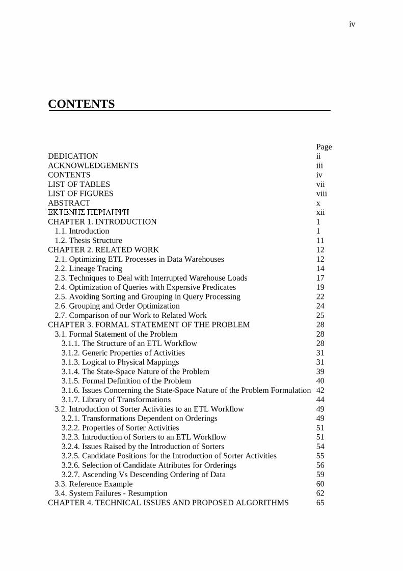
CONTENTS

Page DEDICATION ii ACKNOWLEDGEMENTS iii CONTENTS iv LIST OF TABLES vii LIST OF FIGURES viii ABSTRACT x ΕΚΤΕΝΗΣ ΠΕΡΙΛΗΨΗ xii CHAPTER 1. INTRODUCTION 1

1.1. Introduction 1 1.2. Thesis Structure 11

CHAPTER 2. RELATED WORK 12 2.1. Optimizing ETL Processes in Data Warehouses 12 2.2. Lineage Tracing 14 2.3. Techniques to Deal with Interrupted Warehouse Loads 17 2.4. Optimization of Queries with Expensive Predicates 19 2.5. Avoiding Sorting and Grouping in Query Processing 22 2.6. Grouping and Order Optimization 24 2.7. Comparison of our Work to Related Work 25

CHAPTER 3. FORMAL STATEMENT OF THE PROBLEM 28 3.1. Formal Statement of the Problem 28

3.1.1. The Structure of an ETL Workflow 28 3.1.2. Generic Properties of Activities 31 3.1.3. Logical to Physical Mappings 31 3.1.4. The State-Space Nature of the Problem 39 3.1.5. Formal Definition of the Problem 40 3.1.6. Issues Concerning the State-Space Nature of the Problem Formulation 42 3.1.7. Library of Transformations 44

3.2. Introduction of Sorter Activities to an ETL Workflow 49 3.2.1. Transformations Dependent on Orderings 49 3.2.2. Properties of Sorter Activities 51 3.2.3. Introduction of Sorters to an ETL Workflow 51 3.2.4. Issues Raised by the Introduction of Sorters 54 3.2.5. Candidate Positions for the Introduction of Sorter Activities 55 3.2.6. Selection of Candidate Attributes for Orderings 56 3.2.7. Ascending Vs Descending Ordering of Data 59

3.3. Reference Example 60 3.4. System Failures - Resumption 62

CHAPTER 4. TECHNICAL ISSUES AND PROPOSED ALGORITHMS 65

v

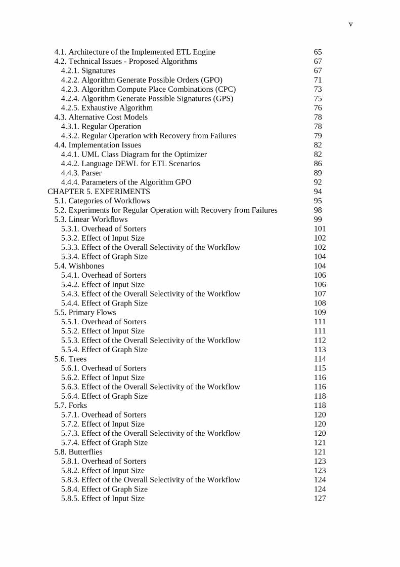
4.1. Architecture of the Implemented ETL Engine 65 4.2. Technical Issues - Proposed Algorithms 67

4.2.1. Signatures 67 4.2.2. Algorithm Generate Possible Orders (GPO) 71 4.2.3. Algorithm Compute Place Combinations (CPC) 73 4.2.4. Algorithm Generate Possible Signatures (GPS) 75 4.2.5. Exhaustive Algorithm 76

4.3. Alternative Cost Models 78 4.3.1. Regular Operation 78 4.3.2. Regular Operation with Recovery from Failures 79

4.4. Implementation Issues 82 4.4.1. UML Class Diagram for the Optimizer 82 4.4.2. Language DEWL for ETL Scenarios 86 4.4.3. Parser 89 4.4.4. Parameters of the Algorithm GPO 92

CHAPTER 5. EXPERIMENTS 94 5.1. Categories of Workflows 95 5.2. Experiments for Regular Operation with Recovery from Failures 98 5.3. Linear Workflows 99

5.3.1. Overhead of Sorters 101 5.3.2. Effect of Input Size 102 5.3.3. Effect of the Overall Selectivity of the Workflow 102 5.3.4. Effect of Graph Size 104

5.4. Wishbones 104 5.4.1. Overhead of Sorters 106 5.4.2. Effect of Input Size 106 5.4.3. Effect of the Overall Selectivity of the Workflow 107 5.4.4. Effect of Graph Size 108

5.5. Primary Flows 109 5.5.1. Overhead of Sorters 111 5.5.2. Effect of Input Size 111 5.5.3. Effect of the Overall Selectivity of the Workflow 112 5.5.4. Effect of Graph Size 113

5.6. Trees 114 5.6.1. Overhead of Sorters 115 5.6.2. Effect of Input Size 116 5.6.3. Effect of the Overall Selectivity of the Workflow 116 5.6.4. Effect of Graph Size 118

5.7. Forks 118 5.7.1. Overhead of Sorters 120 5.7.2. Effect of Input Size 120 5.7.3. Effect of the Overall Selectivity of the Workflow 120 5.7.4. Effect of Graph Size 121

5.8. Butterflies 121 5.8.1. Overhead of Sorters 123 5.8.2. Effect of Input Size 123 5.8.3. Effect of the Overall Selectivity of the Workflow 124 5.8.4. Effect of Graph Size 124 5.8.5. Effect of Input Size 127

vi

5.8.6. Effect of Graph Size 127 5.8.7. Effect of Complexity (Depth and Fan-out) of the Right Wing 127

5.9. Observations Deduced from Experiments 128 CHAPTER 6. CONCLUSIONS AND FUTURE WORK 131

6.1. Conclusions 131 6.2. Future Work 132

REFERENCES 133 APPENDIX 135 SHORT BIOGRAPHICAL SKETCH 136

vii

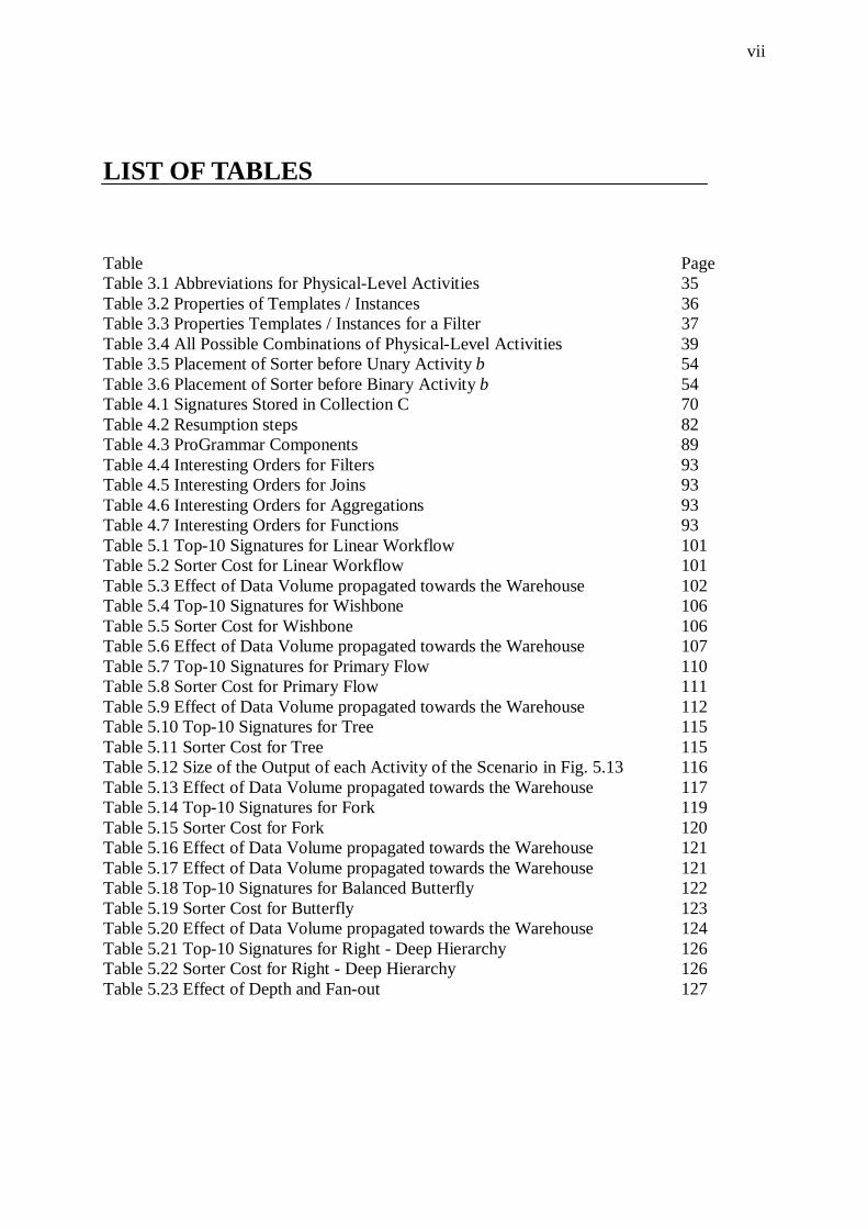
LIST OF TABLES

Table Page Table 3.1 Abbreviations for Physical-Level Activities 35 Table 3.2 Properties of Templates / Instances 36 Table 3.3 Properties Templates / Instances for a Filter 37 Table 3.4 All Possible Combinations of Physical-Level Activities 39 Table 3.5 Placement of Sorter before Unary Activity b 54 Table 3.6 Placement of Sorter before Binary Activity b 54 Table 4.1 Signatures Stored in Collection C 70 Table 4.2 Resumption steps 82 Table 4.3 ProGrammar Components 89 Table 4.4 Interesting Orders for Filters 93 Table 4.5 Interesting Orders for Joins 93 Table 4.6 Interesting Orders for Aggregations 93 Table 4.7 Interesting Orders for Functions 93 Table 5.1 Top-10 Signatures for Linear Workflow 101 Table 5.2 Sorter Cost for Linear Workflow 101 Table 5.3 Effect of Data Volume propagated towards the Warehouse 102 Table 5.4 Top-10 Signatures for Wishbone 106 Table 5.5 Sorter Cost for Wishbone 106 Table 5.6 Effect of Data Volume propagated towards the Warehouse 107 Table 5.7 Top-10 Signatures for Primary Flow 110 Table 5.8 Sorter Cost for Primary Flow 111 Table 5.9 Effect of Data Volume propagated towards the Warehouse 112 Table 5.10 Top-10 Signatures for Tree 115 Table 5.11 Sorter Cost for Tree 115 Table 5.12 Size of the Output of each Activity of the Scenario in Fig. 5.13 116 Table 5.13 Effect of Data Volume propagated towards the Warehouse 117 Table 5.14 Top-10 Signatures for Fork 119 Table 5.15 Sorter Cost for Fork 120 Table 5.16 Effect of Data Volume propagated towards the Warehouse 121 Table 5.17 Effect of Data Volume propagated towards the Warehouse 121 Table 5.18 Top-10 Signatures for Balanced Butterfly 122 Table 5.19 Sorter Cost for Butterfly 123 Table 5.20 Effect of Data Volume propagated towards the Warehouse 124 Table 5.21 Top-10 Signatures for Right - Deep Hierarchy 126 Table 5.22 Sorter Cost for Right - Deep Hierarchy 126 Table 5.23 Effect of Depth and Fan-out 127

viii

LIST OF FIGURES

Figure Page Figure 1.1 Architecture of a Data Warehouse 2 Figure 1.2 Extract - Transform - Load 4 Figure 1.3 A Simple ETL Workflow 6 Figure 2.1 Transformation Classes [CuWi03] 15 Figure 3.1 Illegal Cases for the Interconnection of Activities and Recordsets 30 Figure 3.2 A Logical-Level Activity 33 Figure 3.3 Mapping of a Logical-Level Activity to Physical-Level Activities 33 Figure 3.4 Alternative Physical-Level Activities 34 Figure 3.5 An Example ETL Scenario 38 Figure 3.6 Placement of Sorter on Recordset 53 Figure 3.7 Candidate Positions for Sorters 55 Figure 3.8 Candidate Places for Sorters 56 Figure 3.9 Candidate Sorters 58 Figure 3.10 Candidate Sorters 59 Figure 3.11 An Example ETL Workflow 60 Figure 3.12 Resumption Techniques 62 Figure 4.1 Extract - Transform - Load Process 66 Figure 4.2 ETL engine operations 67 Figure 4.3 Exemplary Scenario 67 Figure 4.4 More Complex Workflows 68 Figure 4.5 Algorithm GSign ([SiVS04]) 69 Figure 4.6 Algorithm Extended GSign 69 Figure 4.7 Several Target Nodes 70 Figure 4.8 Algorithm Generate Possible Orders (GPO) 73 Figure 4.9 Example Scenario 74 Figure 4.10 Algorithm Compute Place Combinations (CPC) 74 Figure 4.11 Algorithm Generate Possible Signatures (GPS) 75 Figure 4.12 Example Scenario 76 Figure 4.13 Algorithm Exhaustive Ordering 77 Figure 4.14 Example of Resumption 81 Figure 4.15 UML Class diagram for the ETL Scenario 85 Figure 4.16 The syntax of DEWL for the four common statements 87 Figure 4.17 An Example ETL Scenario 88 Figure 4.18 An Example ETL Scenario expressed in DEWL 88 Figure 4.19 Generated Parse Tree 91 Figure 5.1 Butterfly Components 96 Figure 5.2 Butterfly Configuration 97 Figure 5.3 Special Butterfly Configurations 99

ix

Figure 5.4 Linear Workflow 100 Figure 5.5 Relationship of Data Volume and Total Cost 104 Figure 5.6 Completion Time of Exhaustive Algorithm 104 Figure 5.7 Wishbone 105 Figure 5.8 Relationship of Join Selectivity and Total Cost 108 Figure 5.9 Completion Time of Exhaustive Algorithm 109 Figure 5.10 Primary Flow 110 Figure 5.11 Relationship of Data Volume and Total Cost 113 Figure 5.12 Completion Time of Exhaustive Algorithm 113 Figure 5.13 Tree 114 Figure 5.14 Relationship of Data Volume and Total Cost 117 Figure 5.15 Completion Time of Exhaustive Algorithm 118 Figure 5.16 Fork 119 Figure 5.17 Butterfly 122 Figure 5.18 Completion Time of Exhaustive Algorithm 125 Figure 5.19 Right - Deep Hierarchy 125 Figure A.1 Butterfly (Sum of pi is 1%) 135 Figure A.2 Butterfly (Sum of pi is 5%) 135 Figure A.3 Butterfly (Sum of pi is 10%) 135

x

ABSTRACT

Tziovara, Vasiliki, A. MSc, Computer Science Department, University of Ioannina, Greece. October, 2006. Order-Aware ETL Workflows. Thesis Supervisor: Panos Vassiliadis. Data Warehouses are collections of data coming from different sources, used mostly to

support decision making and data analysis in an organization. To populate a data warehouse

with up-to-date records that are extracted from the sources, special tools are employed, called

Extraction – Transform – Load (ETL) tools, which organize the steps of the whole process as

a workflow. An ETL workflow can be considered as a directed acyclic graph (DAG) used to

capture the flow of data from the sources to the data warehouse. The nodes of the graph are

activities that apply transformations or cleansing procedures on data or recordsets used for

storage purposes. The edges of the graph are input/output relationships between the nodes.

The workflow is an abstract design at the logical level, which has to be implemented

physically, i.e., to be mapped to a combination of executable programs/scripts that perform

the ETL workflow. Each activity of the workflow can be implemented physically using

various algorithmic methods, each with different cost in terms of time requirements or system

resources (e.g., memory, space on disk, etc.).

The objective of this work is to identify the best possible implementation of a logical ETL

workflow. For this reason, we employ (a) a library of templates for the activities and (b) a set

of mappings between logical and physical templates. First, we use a simple cost model, that

computes as optimal, the scenario with the best expected execution speed. In this work, we

model the problem as a state-space search problem and propose an exhaustive algorithm for

state generation to discover the optimal physical implementation of the scenario. To this end,

we propose a cost model as a discrimination criterion between physical representations, which

works also for black-box activities with unknown semantics. We also study the effects of

possible system failures to the workflow operation. The difficulty in this case, lies at the

xi

computation of the cost of the workflow in case of failures. Therefore, we propose a different

cost model that works for the case of failures. To further reduce the total cost of the scenario,

we introduce an additional set of special-purpose activities, called sorter activities which

apply on stored recordsets and sort their tuples according to the values of some, critical for the

sorting, attributes.

In addition, we provide a set of template structures for workflows, to which we refer as

butterflies because of the shape of their graphical representation. Finally, we assess the

performance of the proposed algorithm through a set of experimental results.

xii

ΕΚΤΕΝΗΣ ΠΕΡΙΛΗΨΗ

Βασιλική Τζιοβάρα του Αχιλλέα και της Σπυριδούλας. MSc, Τμήμα Πληροφορικής, Πανεπιστήμιο Ιωαννίνων, Ελλάδα. Οκτώβριος, 2006. Ταξινόμηση σε Ροές Εργασίας Αποθηκών Δεδομένων. Επιβλέποντας: Παναγιώτης Βασιλειάδης. Οι Αποθήκες Δεδομένων είναι συλλογές δεδομένων που προέρχονται από διαφορετικές πηγές

και χρησιμοποιούνται κυρίως για τη λήψη αποφάσεων σε ένα οργανισμό. Για να

τροφοδοτηθεί μια αποθήκη με νέα δεδομένα, όπως αυτά παράγονται στις πηγές,

χρησιμοποιούνται εργαλεία Εξαγωγής – Μετασχηματισμού – Φόρτωσης δεδομένων (Extract

– Transform – Load tools, ETL), τα οποία οργανώνουν τα επί μέρους βήματα της όλης

διαδικασίας σαν μια ροή εργασίας. Μια ροή εργασίας ETL μπορεί να θεωρηθεί ως ένας

κατευθυνόμενος ακυκλικός γράφος (DAG) που χρησιμοποιείται για να αναπαραστήσει τη

ροή δεδομένων από τις πηγές δεδομένων προς την αποθήκη δεδομένων. Οι κόμβοι του

γράφου είναι διαδικασίες καθαρισμού/ μετασχηματισμού δεδομένων ή σύνολα εγγραφών και

οι ακμές σχέσεις εισόδου/εξόδου μεταξύ των κόμβων. Η ροή εργασίας είναι ένα αφηρημένο

σχήμα σε λογικό επίπεδο, το οποίο πρέπει να υλοποιηθεί σε φυσικό επίπεδο, δηλαδή να

αντιστοιχηθεί σε ένα συνδυασμό από εκτελέσιμα προγράμματα που εκτελούν την ETL ροή

εργασίας. Κάθε διαδικασία της ροής εργασίας μπορεί να υλοποιηθεί με ποικίλες αλγοριθμικές

μεθόδους, καθεμιά με διαφορετικό κόστος όσον αφορά απαιτήσεις σε χρόνο ή πόρους

συστήματος (π.χ., μνήμη, χώρο στο δίσκο, κλπ.).

Ο σκοπός αυτής της εργασίας είναι να εντοπίσουμε την καλύτερη δυνατή υλοποίηση ενός

λογικού γράφου ETL. Για το σκοπό αυτό, χρειαζόμαστε (α) μια βιβλιοθήκη από πρότυπα για

τις διαδικασίες και (β) αντιστοιχίσεις μεταξύ λογικών και φυσικών προτύπων. Αρχικά

ξεκινούμε με ένα απλό μοντέλο κόστους, που υπολογίζει ως βέλτιστο, το σενάριο εκτέλεσης

με την καλύτερη αναμενόμενη ταχύτητα εκτέλεσης. Σε αυτή την εργασία, για να εντοπίσουμε

τη βέλτιστη υλοποίηση ενός λογικού γράφου ETL, μοντελοποιούμε το πρόβλημα ως

xiii

πρόβλημα αναζήτησης σε χώρο καταστάσεων και προτείνουμε έναν εξαντλητικό αλγόριθμο

καταστάσεων. Επίσης, προτείνουμε ένα μοντέλο κόστους ως κριτήριο διάκρισης μεταξύ

φυσικών αναπαραστάσεων, το οποίο χαρακτηρίζεται από την καταλληλότητά του για

δομήσεις λογισμικού με την τεχνική του μαύρου κουτιού και τη χρήση έτοιμων συστατικών

στοιχείων λογισμικού ως κόμβων του γράφου.

Επιπρόσθετα της κανονικής λειτουργίας, μελετάμε τις επιπτώσεις στη λειτουργία της ροής

εργασίας από πιθανές αποτυχίες του συστήματος. Η δυσκολία του προβλήματος εντοπίζεται

στον υπολογισμό του κόστους λόγω των αποτυχιών και, κατά συνέπεια, προτείνουμε ένα

διαφορετικό μοντέλο κόστους που περιλαμβάνει και τις περιπτώσεις αποτυχιών.

Επιπλέον, με σκοπό να μειωθεί περαιτέρω το κόστος του γράφου, εισάγουμε ένα επιπρόσθετο

σύνολο διαδικασιών που ταξινομούν κάποια από τα εμπλεκόμενα σύνολα εγγραφών

σύμφωνα με τις τιμές κάποιων, κρίσιμων για την ταξινόμηση, πεδίων.

Τέλος, οργανώνουμε τις ροές εργασίας σε πρότυπες δομές, τις οποίες ονομάζουμε

«πεταλούδες» (λόγω του σχήματος της γραφικής τους αναπαράστασης) και ελέγχουμε

πειραματικά την απόδοση του προτεινόμενου αλγορίθμου για διαφορετικές κατηγορίες

πεταλούδων.

1

CHAPTER 1. INTRODUCTION

1.1 Introduction

1.2 Thesis Structure

1.1. Introduction

A Data Warehouse (DW) is an information infrastructure that collects, integrates and stores

an organization's data. The most important feature of a Data Warehouse is that it produces

accurate and timely management information, so companies utilize data warehouses to enable

their employees (executives, managers, analysts, etc.) to make better and faster decisions.

Furthermore, data warehouses can be used to support complex data analysis. According to

Inmon [Inmo02], a DW is “a collection of subject-oriented, integrated, non-volatile and time-

variant data in support of management decisions”.

W. H. Inmon [Inmo02] presents a formal definition of a data warehouse as a database

consisting of computerized data that is organized to most optimally support reporting and

analysis activity. According to Inmon, a data warehouse has four characteristics:

1. It is subject-oriented, meaning that the data in the DW is organized so that all data

elements relating to the same real-world event or object are linked together.

2. Integrated, meaning that the database contains data from most or all of an

organization’s operational applications, and that this data is gathered in a single

location to be made consistent.

3. Non-volatile, meaning that data in the database is never over-written or deleted, but

retained for future reporting.

2

4. Time-variant, meaning that the changes to the data in the database are tracked and

recorded so that reports can be produced showing changes over time.

There are many advantages of using a data warehouse. First of all, a data warehouse is able to

combine a variety of data from different sources in a single location. Interesting information is

extracted from various distributed sources, which are usually heterogeneous. This means that

the same data is represented differently at the sources, for instance through different database

schemata. The data warehouse has to identify same entities, represented in different ways at

the sources, and model it under a unique database schema. This means that data in a data

warehouse have to go through a series of transformations to be made consistent and up-to-

date. This process is often referred to as semantic reconciliation and is an important property

of the data warehouse. Another advantage of a data warehouse is that it can support changes

to data, since modifications to the data in a data warehouse are tracked and recorded. The data

warehouse also keeps a historical record of the loaded data. Finally, data quality is an

important issue, since data arriving at the data warehouse are in most cases inconsistent. The

above features of a data warehouse show that a data warehouse is always expected to contain

up-to-date, consistent and integrated data in order to support decision making and data

analysis.

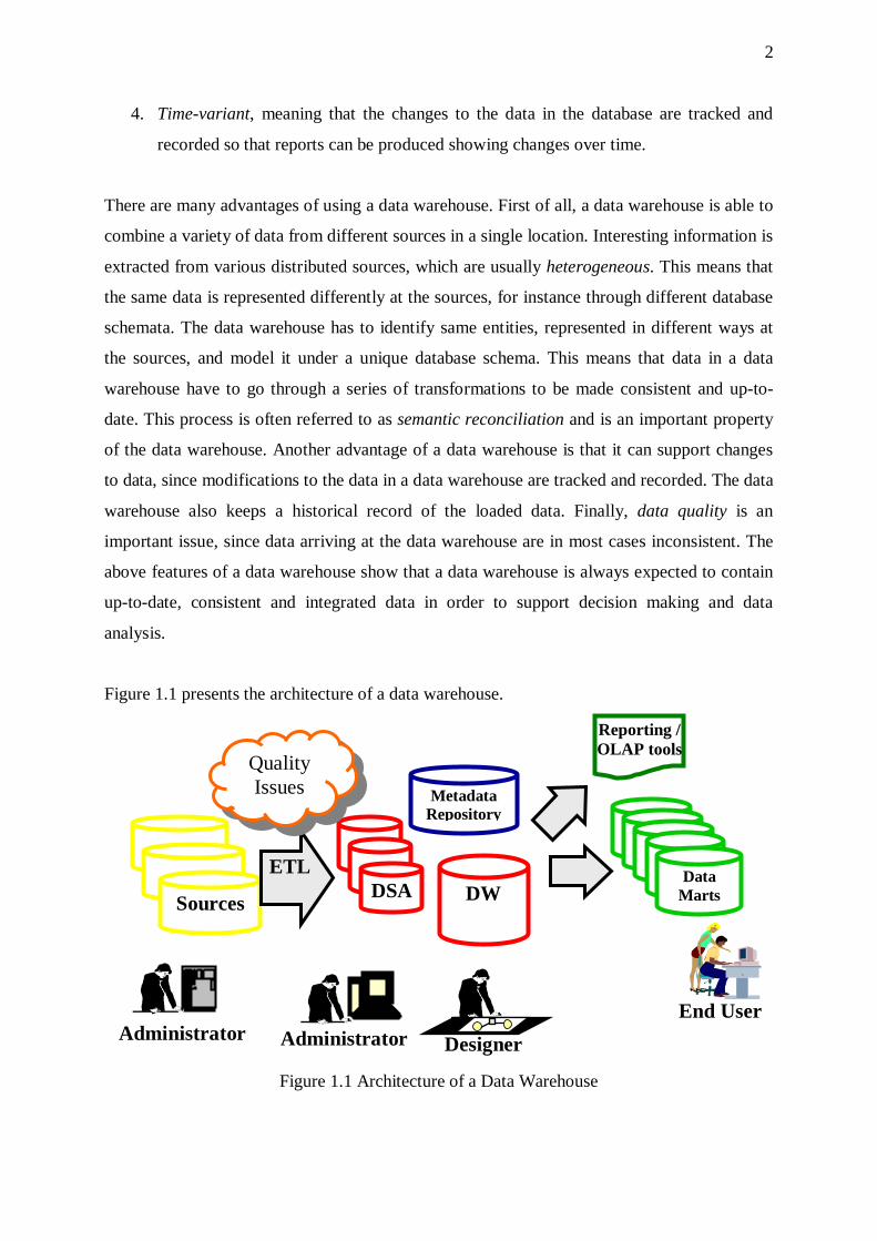
Figure 1.1 presents the architecture of a data warehouse.

Figure 1.1 Architecture of a Data Warehouse

Sources

Administrator

DSA

Administrator

DW

Designer

ETL Data Marts

Metadata Repository

End User

Reporting / OLAP tools

Quality Issues

3

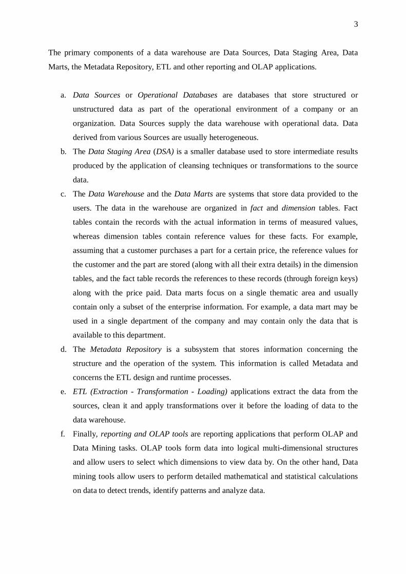
The primary components of a data warehouse are Data Sources, Data Staging Area, Data

Marts, the Metadata Repository, ETL and other reporting and OLAP applications.

a. Data Sources or Operational Databases are databases that store structured or

unstructured data as part of the operational environment of a company or an

organization. Data Sources supply the data warehouse with operational data. Data

derived from various Sources are usually heterogeneous.

b. The Data Staging Area (DSA) is a smaller database used to store intermediate results

produced by the application of cleansing techniques or transformations to the source

data.

c. The Data Warehouse and the Data Marts are systems that store data provided to the

users. The data in the warehouse are organized in fact and dimension tables. Fact

tables contain the records with the actual information in terms of measured values,

whereas dimension tables contain reference values for these facts. For example,

assuming that a customer purchases a part for a certain price, the reference values for

the customer and the part are stored (along with all their extra details) in the dimension

tables, and the fact table records the references to these records (through foreign keys)

along with the price paid. Data marts focus on a single thematic area and usually

contain only a subset of the enterprise information. For example, a data mart may be

used in a single department of the company and may contain only the data that is

available to this department.

d. The Metadata Repository is a subsystem that stores information concerning the

structure and the operation of the system. This information is called Metadata and

concerns the ETL design and runtime processes.

e. ETL (Extraction - Transformation - Loading) applications extract the data from the

sources, clean it and apply transformations over it before the loading of data to the

data warehouse.

f. Finally, reporting and OLAP tools are reporting applications that perform OLAP and

Data Mining tasks. OLAP tools form data into logical multi-dimensional structures

and allow users to select which dimensions to view data by. On the other hand, Data

mining tools allow users to perform detailed mathematical and statistical calculations

on data to detect trends, identify patterns and analyze data.

4

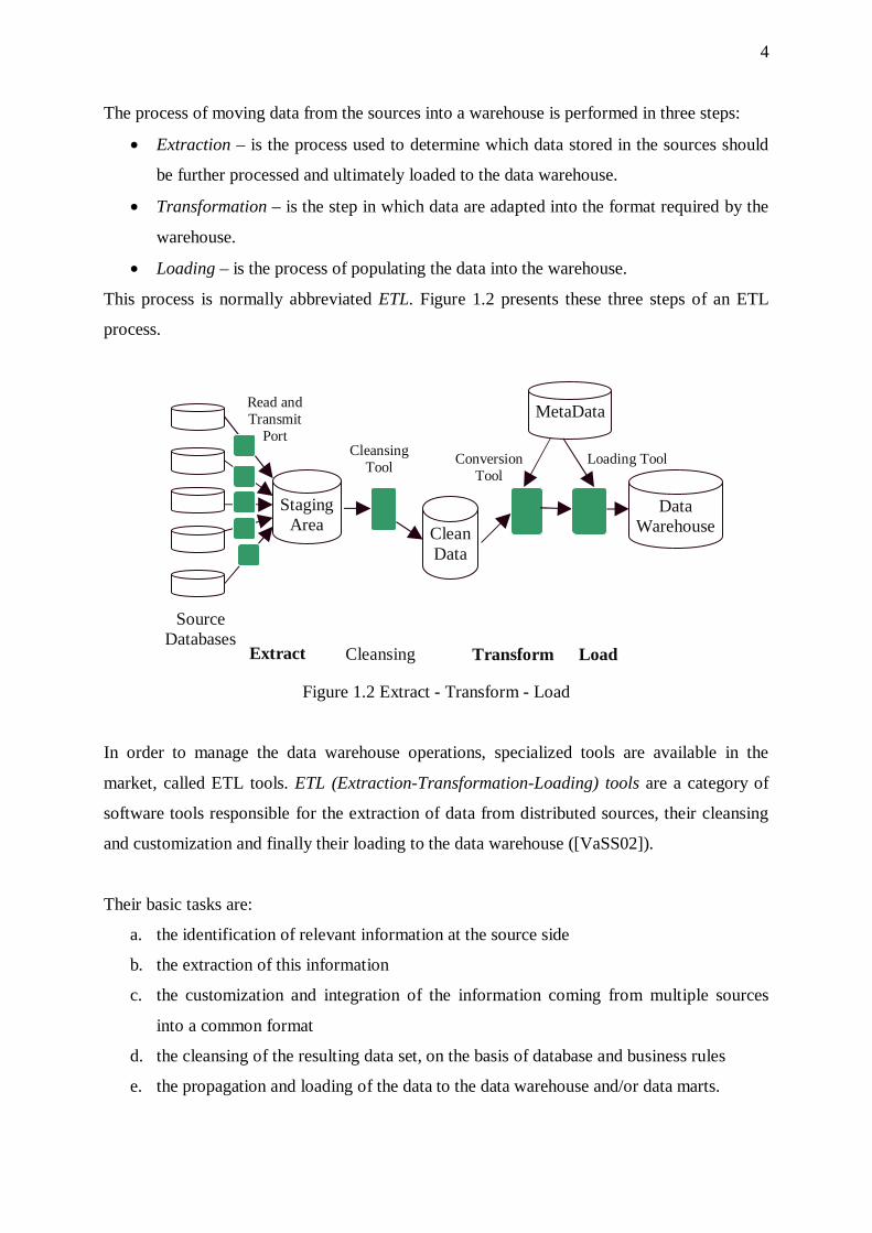
The process of moving data from the sources into a warehouse is performed in three steps:

• Extraction – is the process used to determine which data stored in the sources should

be further processed and ultimately loaded to the data warehouse.

• Transformation – is the step in which data are adapted into the format required by the

warehouse.

• Loading – is the process of populating the data into the warehouse.

This process is normally abbreviated ETL. Figure 1.2 presents these three steps of an ETL

process.

Figure 1.2 Extract - Transform - Load

In order to manage the data warehouse operations, specialized tools are available in the

market, called ETL tools. ETL (Extraction-Transformation-Loading) tools are a category of

software tools responsible for the extraction of data from distributed sources, their cleansing

and customization and finally their loading to the data warehouse ([VaSS02]).

Their basic tasks are:

a. the identification of relevant information at the source side

b. the extraction of this information

c. the customization and integration of the information coming from multiple sources

into a common format

d. the cleansing of the resulting data set, on the basis of database and business rules

e. the propagation and loading of the data to the data warehouse and/or data marts.

Source Databases

Staging Area Clean

Data

MetaData

Extract Cleansing

Cleansing Tool

Data Warehouse

Transform Load

Conversion Tool

Loading Tool

Read and Transmit

Port

5

As we mentioned earlier, in data warehousing, data are extracted from various sources and

have to go through a set of transformations and cleansing procedures before they reach their

destination, usually a data warehouse and/or data marts. Typical data transformations are data

conversions (e.g., conversions from European formats to American and vice versa), orderings

of data, generation of summaries of data (in other words groupings), etc. Finally, data are

loaded into the data warehouse. A typical load of data involves processing large volumes of

data (e.g., several GBs of data) and requires many complex transformations of data. This

means that this process is time-consuming (often takes many hours or even days to complete)

and usually takes place during the night, in order to avoid overloading the system with extra

workload. Moreover, in many systems, the warehouse load must be completed within a

certain time window, which means that the request for performance is pressing. Based on the

above, we can summarize the main problems of ETL tasks: (a) the enormous volumes of data

for processing, (b) performance, since all operations must be completed within a specific

period of time, (c) quality problems, since data usually have to be cleansed. Furthermore, (d)

failures during the transformation process or the warehouse loading process, cause significant

problems to the warehouse operation and finally, (e) the evolution of the sources and the data

warehouse can lead to daily maintenance operations. Under these conditions, we see that we

can overcome the problems of ETL tasks by designing and managing ETL tasks efficiently.

In our setting, we start with a rigorous, abstract modeling of ETL scenarios, based on the

logical model of [VaSS02]. The main idea is that each individual transformation or cleansing

task is treated as an activity in a workflow. An ETL workflow represents graphically the

interconnections among the constituent transformations of an ETL scenario and models the

flow of data from the sources to the warehouse, through these transformations. In our

deliberations, we will refer to workflows as scenarios, too. The two terms will be used

interchangeably. In our approach, we model an ETL workflow as a directed acyclic graph

(DAG) that consists of two kinds of nodes: activities and recordsets. Activities are software

modules that perform transformations or cleansing procedures over data, while recordsets are

used for data storage purposes. Furthermore, the edges of the graph are used to capture the

flow of data from the sources to the data warehouse.

Recordsets can be distinguished in the following broad categories, as described analytically in

[JLVV00]:

6

a. Data Sources or Operational Databases: Databases that store structured or

unstructured data as part of the operational environment of a company or an

organization. Data are collected from the Sources and go through a number of

transformations before they reach the Data Warehouse.

b. DSA (Data Staging Area): Smaller recordsets used to store intermediate results

produced by the application of transformations to the source data.

c. Targets: The transformed data are guided towards one or more destinations, called

Targets. Each target is a repository used for data storage. One of the targets is a central

repository called a Data Warehouse. Data Warehouses hold large amounts of data

(Terabytes of data) and typical warehouse loads range from 1 to 100 GB and take

many hours or even days to execute. Other targets may be materialized views, which

are the stored results of pre-computed user queries. Later queries that need this data

automatically use the materialized views, thus saving the overhead of asking again the

entire data warehouse. Materialized views usually increase the speed of subsequent

queries by many orders of magnitude.

Source databases and DSA Tables can have one or more outputs, since the same data can be

forwarded towards one or more destination. DSA and Target Tables can receive only one data

stream as input.

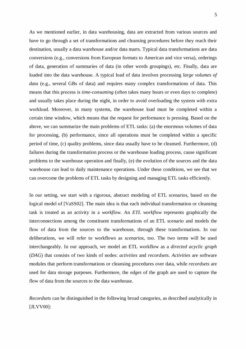
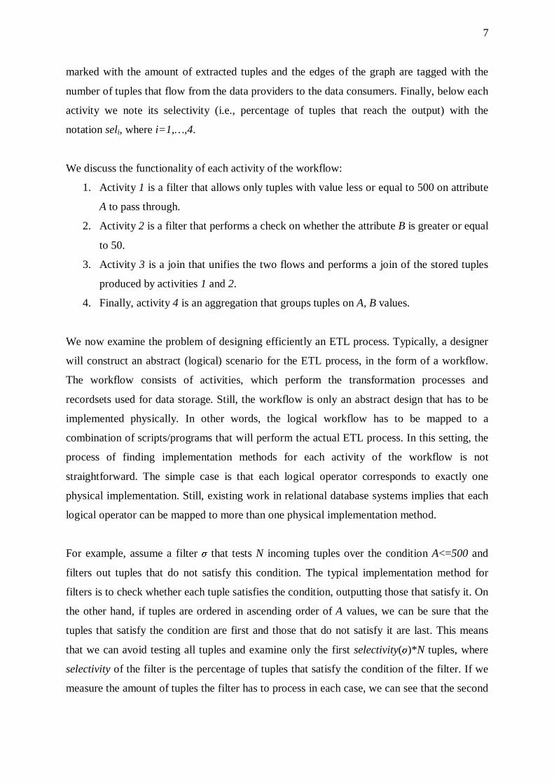
Figure 1.3 A Simple ETL Workflow

Figure 1.3 presents a simple ETL scenario. This scenario involves (a) two source recordsets R

and S, (b) a central data warehouse DW and (c) three DSA tables V, T and Z. The schemata of

the source data are R(A, B) and S(A, B) respectively. Activities are annotated with numbers

from 1 to 4 and tagged with the description of their functionality. Furthermore, the sources are

7

marked with the amount of extracted tuples and the edges of the graph are tagged with the

number of tuples that flow from the data providers to the data consumers. Finally, below each

activity we note its selectivity (i.e., percentage of tuples that reach the output) with the

notation seli, where i=1,…,4.

We discuss the functionality of each activity of the workflow:

1. Activity 1 is a filter that allows only tuples with value less or equal to 500 on attribute

A to pass through.

2. Activity 2 is a filter that performs a check on whether the attribute B is greater or equal

to 50.

3. Activity 3 is a join that unifies the two flows and performs a join of the stored tuples

produced by activities 1 and 2.

4. Finally, activity 4 is an aggregation that groups tuples on A, B values.

We now examine the problem of designing efficiently an ETL process. Typically, a designer

will construct an abstract (logical) scenario for the ETL process, in the form of a workflow.

The workflow consists of activities, which perform the transformation processes and

recordsets used for data storage. Still, the workflow is only an abstract design that has to be

implemented physically. In other words, the logical workflow has to be mapped to a

combination of scripts/programs that will perform the actual ETL process. In this setting, the

process of finding implementation methods for each activity of the workflow is not

straightforward. The simple case is that each logical operator corresponds to exactly one

physical implementation. Still, existing work in relational database systems implies that each

logical operator can be mapped to more than one physical implementation method.

For example, assume a filter σ that tests N incoming tuples over the condition A<=500 and

filters out tuples that do not satisfy this condition. The typical implementation method for

filters is to check whether each tuple satisfies the condition, outputting those that satisfy it. On

the other hand, if tuples are ordered in ascending order of A values, we can be sure that the

tuples that satisfy the condition are first and those that do not satisfy it are last. This means

that we can avoid testing all tuples and examine only the first selectivity(σ)*N tuples, where

selectivity of the filter is the percentage of tuples that satisfy the condition of the filter. If we

measure the amount of tuples the filter has to process in each case, we can see that the second

8

implementation method requires the testing of fewer tuples. As a result, this method is

beneficial in terms of processing time.

Taking into consideration all the possible implementation methods available for each logical

activity, we can see that the selection of which physical implementation should be applied for

each logical activity of the workflow is a difficult problem. This problem becomes even more

complicated because of the interactions between activities. This means that the

implementation method selected for an activity affects the selection of the implementation

methods for the subsequent activities of the workflow. For example, assume an activity that

performs a Sort-Merge Join followed by an aggregation. Since the output tuples of a Sort-

Merge Join are ordered according to the join attribute, the aggregation could be implemented

using a Sort-based algorithm that exploits this ordering rather than a Nested-Loops

implementation. Thus, the choice of the implementation method for the second activity (i.e.,

the aggregation) depends on the physical implementation of the first one.

Finally, the same problem of logical-to-physical mappings occurs if instead of deciding which

implementation algorithm to use for each logical operator, we have some available libraries of

templates for activities. Assume a library of logical templates and a library of physical

templates. In this case, we map each logical operator to a logical-level template from the

library. Then, we employ logical-to-physical mappings at the template level to map the logical

template to a set of physical templates. Finally, we customize each physical template to a

physical activity, taking into consideration all physical-level constraints.

Since ETL processes handle large volumes of data, the management of such a workload is a

complex and expensive operation in terms of time and system resources. Therefore, the

minimization of the resources needed for ETL tasks and the elimination of the time

requirements for their completion present a problem with clear practical consequences.

Therefore, we need to identify the optimal configuration, in terms of performance gains, out

of all the computed physical representations of the workflow. In this work, we are interested

in the optimization of an ETL scenario, i.e., in the minimization of the cost of the scenario.

We will refer to this cost as the total cost of the scenario. We consider ways to minimize the

total cost of an ETL scenario. For this reason, we investigate all possible physical

9

implementations of a given ETL scenario and discover the one that is more profitable in terms

of time or consumption of system resources.

So far, research work has only partly dealt with the aforementioned problem. For the moment,

research approaches have focused on different topics, such as query optimization. The first

paper to address this problem was the paper of P. Selinger et al [SAC+79] that dealt with

query optimization techniques. This problem is one of the issues an optimizer has to address

during the evaluation of queries. Part of the optimizer’s job is to produce one or more

interesting orders, i.e., a set of ordering specifications that can be useful for the query

rewriting and the generation of a plan with lower cost.

Other approaches are concerned with order optimization, which refers to the subarea of plan

generation that is concerned with handling interesting orders. Later papers ([SiSM96],

[Hell98], [WaCh03]) have mainly focused on techniques to “push down”, combine or exploit

existing orders in query plans. These papers focus on relational queries and do not handle

ETL processes. ETL processes cannot be considered as “big” queries, since there are

processes that run in separate environments, usually not simultaneously and under time

constraints. Thus, the traditional techniques for query optimization can be blocked, due to

data-manipulation functions.

Furthermore, many of the studies employ interesting orders, but rely on functional

dependencies ([SiSM96], [NeMo04]) and predicates applied over data. Some work has been

done on exploiting existing orderings and groupings. For example, Wang and Cherniack

([WaCh03]) recognize that orderings and groupings are expensive operations and propose the

exploitation of existing operators for the pruning of redundant orderings and groupings. Most

of these papers are discussed systematically in Chapter 2, as part of the Related Work. To our

knowledge, none of the above approaches consider the introduction of new orderings.

On the other hand, leading commercial tools allow the design of ETL workflows, but do not

use any optimization technique. Few ETL tools employ optimization methods, such as Arktos

II [Arkt05]. Arktos II not only allows the logical design of an ETL scenario, but also the

physical representation of ETL tasks. Furthermore, Arktos II takes into consideration the

optimization of ETL scenarios and tries to improve the time performance of ETL processes.

10

The objective of this work is to discover the best possible physical implementation of a given

logical ETL workflow. For this reason, we need (a) a library of templates for the activities and

(b) possible mappings between logical and physical templates. As a first approach, we employ

a simple cost model that computes as optimal, the scenario with the best expected execution

speed. To discover the optimal physical implementation of the scenario, we model the

problem as a state-search space problem and propose an exhaustive algorithm for state

generation. To identify the optimal physical representation of the scenario, we propose a cost

model as a discrimination criterion between physical representations, which works also for

black-box activities with unknown semantics. We also study the effects of possible system

failures to the workflow operation. The difficulty in this case, lies in the computation of the

cost of the workflow in case of failures. Therefore, we propose a different cost model that

works for the case of failures. In addition, to further reduce the total cost of the scenario we

introduce an additional set of special-purpose activities, called sorter activities which apply

on stored recordsets and sort their tuples according to the values of some, critical for the

sorting, attributes.

In the absence of a standard way to perform experiments on the topic, we organize our

experiments on the basis of a reference collection of ETL scenarios. Each such scenario is a

variant of a template workflow structure, which we call Butterfly, due to its shape when

depicted graphically. A butterfly comprises a left wing, where data coming from different

sources are combined in order to populate a fact table in the warehouse. This fact table is

called body of the butterfly. The right wing involves the refreshment of materialized views

lying in the warehouse.

Finally, we experimentally assess the performance of the proposed algorithm on different

categories of butterflies.

Our contributions can be summarized as follows:

• We provide a theoretical framework for the problem of mapping a logical ETL

workflow to alternative physical representations.

• We implement an exhaustive algorithm that generates all possible physical

representations of a given ETL scenario and returns the one having minimal cost.

11

• We study the effects of system failures to the workflow operation and propose an

extended cost model for the case of failures.

• We devise a method that can further reduce the execution cost of an ETL workflow by

introducing sorter activities to certain positions of the workflow.

• We provide a set of template structures for workflows, to which we refer as Butterflies

because of the shape of their graphical representation.

• Finally, we discuss technical issues and assess our approach through a set of

experimental results.

1.2. Thesis Structure

This thesis is organized as follows: Chapter 2 presents Related Work and its shortcomings

with respect to the problem we are interested in. In Chapter 3 we model the problem as a

state-space search problem and present the formal statement of the problem. Furthermore, we

discuss the mapping of a logical-level ETL scenario to alternative physical-level scenarios.

Then, we present the generic properties of activities and a library of templates for ETL

activities. As a method to further reduce the cost of an ETL workflow, we propose the

exploitation of interesting orders and the introduction of sorter activities to the workflow. In

Chapter 4 we discuss implementation issues and present the exhaustive algorithm. This

algorithm along with different cost models are experimentally assessed in Chapter 5. In

addition, we organize workflows into template structures, called butterflies. Finally, in

Chapter 6 we summarize our results and discuss interesting issues for future research.

12

CHAPTER 2. RELATED WORK

2.1 Optimizing ETL Processes in Data Warehouses

2.2 Lineage Tracing

2.3 Techniques to Deal with Interrupted Warehouse Loads

2.4 Optimization of Queries with Expensive Predicates

2.5 Avoiding Sorting and Grouping in Query Processing

2.6 Grouping and Order Optimization

2.7 Comparison of our Work to Related Work

2.1. Optimizing ETL Processes in Data Warehouses

In section 1.1, we explained that ETL (Extraction - Transformation - Loading) tools are

software tools responsible for the extraction of data from different sources, their cleansing,

transformation and insertion into a data warehouse. This course of action must be completed

within certain time limits. Thus, the minimization of the execution time of the above

processes presents a research problem with clear practical consequences. The authors of

[SiVS05] model an ETL workflow as a Directed Acyclic Graph (DAG), whose nodes are

activities or recordsets and whose edges represent the flow of data through the graph nodes.

The authors handle the problem of the optimization of an ETL workflow, i.e., minimizing its

execution cost, as a state-space search problem. Every ETL workflow is considered as a state.

Equivalent states are assumed to be states that based on the same input, provide the same

output. The authors propose some transformations that can be applied to the graph nodes to

produce new equivalent states, called transitions. They introduce five transitions: Swap,

Factorize, Distribute, Merge and Split and the corresponding notations.

• Swap: This transition is applied to a pair of unary activities by exchanging their

position in the workflow. Swapping is conducted with the aim of pushing highly

13

selective activities towards the beginning of the workflow (same as in query

optimization). Thus, there is a reduction in the number of tuples that have to be

processed.

• Factorize: Factorize replaces two unary activities that (a) have the same functionality

and (b) act as the two providers of the same binary activity with a new unary activity,

which is placed after the binary activity. Factorization is performed in order to exploit

the fact that a certain operation is performed only once instead of twice in a workflow,

possibly over fewer data.

• Distribute: This transition is the reciprocal of Factorize. If an activity operates over a

single data flow, it can be distributed into two different data flows. For example,

distribution is conducted if an activity is highly selective. In this way, highly selective

activities are pushed towards the beginning of the workflow.

• Merge: Merge is applied over a pair of activities, which are combined into a single

activity. Merge is performed when some activities have to be grouped according to the

constraints of the workflow, e.g., a third activity cannot be placed between this pair of

activities or these two activities cannot be commuted.

• Split: This transition indicates that a pair of grouped activities can be ungrouped and

separates the activities.

The problem of the “optimization of an ETL workflow” involves the discovery of a state

equivalent to the given one, which has the minimal execution cost. Furthermore, the authors

prove the correctness of the proposed transitions and make a reference to cases where each of

these transitions can be applied. Then, a cost model is introduced and the following

optimization algorithms of the ETL processes are presented: the exhaustive algorithm ES, the

heuristic algorithm HS that reduces the search space and a greedy variation of the heuristic

algorithm.

1. The exhaustive algorithm ES works as follows: We generate all the possible states that

can be generated by applying all the applicable transitions to every state.

2. The heuristic algorithm HS involves the following steps:

• Pre-Processing: Use Merge before any other transition.

• Phase 1: Use Swap only in linear paths.

• Phase 2: Factorize only homologous activities placed in two converging paths.

14

• Phase 3: Distribute only if transformation is applicable.

• Phase 4: Swap again only in the linear paths of the new states produced in phases

‘2’ and ‘3’.

3. The Greedy variant of the Heuristic search works as follows:

• Apply Swap only if we gain in cost.

Finally, the authors compare the performance of the three algorithms, and present relative

experimental results. The ES algorithm was slower compared to the other two and in most

cases it could not terminate due to the exponential size of the search space. As a threshold, ES

run up to 40 hours. For small workflows, although both HS and HS-Greedy provide solutions

of approximately the same quality, HS-Greedy was faster at least 86%. For medium

workflows, HS finds better solution than HS-Greedy, while HS-Greedy is much faster than

HS. In large test cases, HS has an advantage because it returns workflows with much

improved cost, whereas HS-Greedy returns unstable results in approximately half of the test

cases.

2.2. Lineage Tracing

Data warehousing systems collect large amounts of data from different data sources into a

central warehouse. During this process, source data go through a series of transformations,

which may vary from simple algebraic operations (such as selections or joins) or aggregations

to complex data cleansing procedures. In [CuWi03] the authors handle the data lineage

problem, which means tracing certain warehouse data items back to the original source items

from which they were derived. During this process, it is useful to look not only at the

information in the warehouse, but also to investigate how these items were derived from the

sources. The tracing procedure takes advantage of any known structure or properties of

transformations but can also work in the absence of such information and provide tracing

facilities.

A data set is defined as a set of data items (tuples, values or complex objects) with no

duplicates in the set. A transformation T is a procedure that applies to one or more datasets

and produces one or more datasets as output. Then, the authors present some basic properties

of transformations, which are the following:

15

• A transformation T is stable if it never produces spurious output items, i.e., if it never

produces datasets as output without taking any datasets as input. An example of an

unstable transformation is one that appends a fixed data set or set of items to every

output set, regardless of the input.

• A transformation T is deterministic if it always produces the same output set given the

same input set.

• A transformation T is complete if each input data item always contributes to some

output data item.

The authors assume that all transformations employed in their work are stable and

deterministic. Another useful term is the lineage of an output item o, which is described as the

actual set I* of input items I that contribute to o’s derivation and is denoted as I*=T*(o, I).

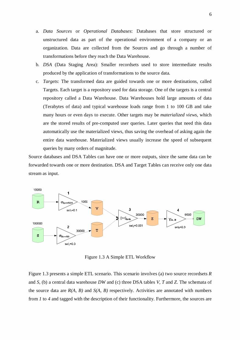
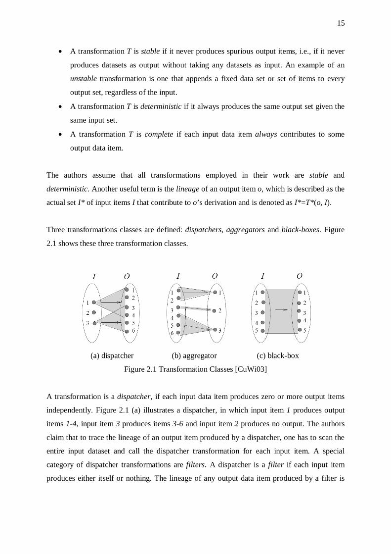
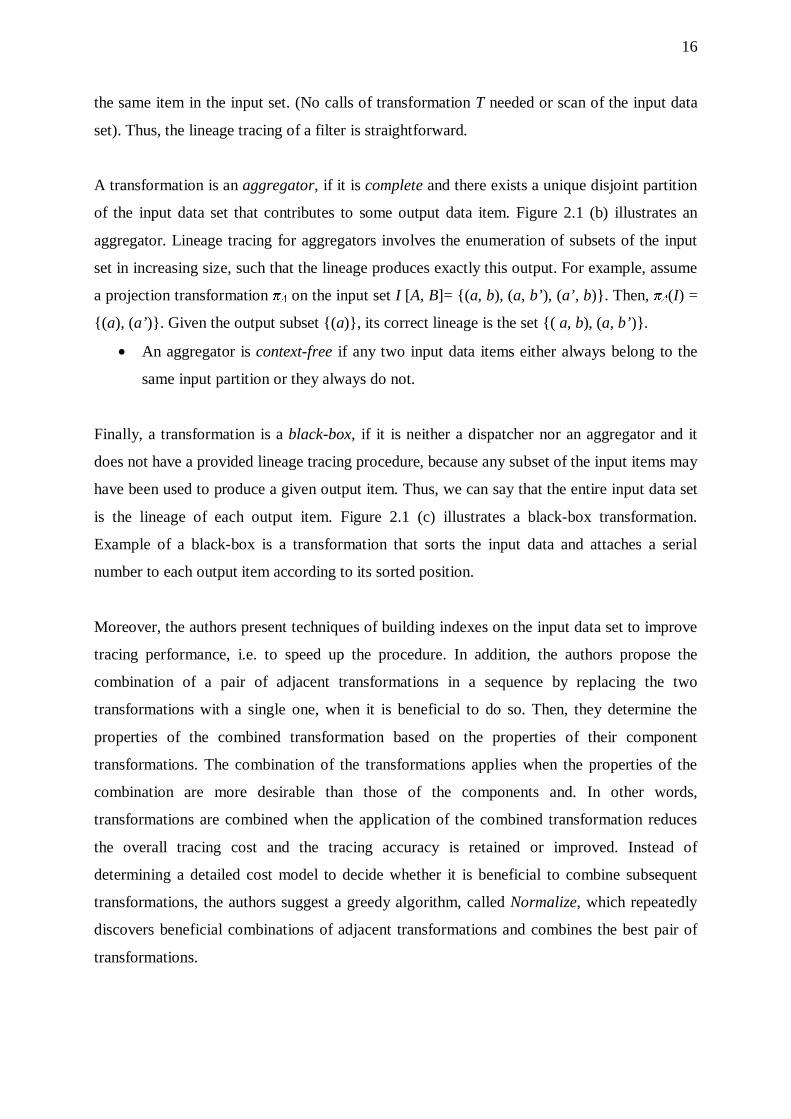
Three transformations classes are defined: dispatchers, aggregators and black-boxes. Figure

2.1 shows these three transformation classes.

(a) dispatcher (b) aggregator (c) black-box

Figure 2.1 Transformation Classes [CuWi03]

A transformation is a dispatcher, if each input data item produces zero or more output items

independently. Figure 2.1 (a) illustrates a dispatcher, in which input item 1 produces output

items 1-4, input item 3 produces items 3-6 and input item 2 produces no output. The authors

claim that to trace the lineage of an output item produced by a dispatcher, one has to scan the

entire input dataset and call the dispatcher transformation for each input item. A special

category of dispatcher transformations are filters. A dispatcher is a filter if each input item

produces either itself or nothing. The lineage of any output data item produced by a filter is

16

the same item in the input set. (No calls of transformation T needed or scan of the input data

set). Thus, the lineage tracing of a filter is straightforward.

A transformation is an aggregator, if it is complete and there exists a unique disjoint partition

of the input data set that contributes to some output data item. Figure 2.1 (b) illustrates an

aggregator. Lineage tracing for aggregators involves the enumeration of subsets of the input

set in increasing size, such that the lineage produces exactly this output. For example, assume

a projection transformation πΑ on the input set I [A, B]= (a, b), (a, b’), (a’, b). Then, πΑ(I) =

(a), (a’). Given the output subset (a), its correct lineage is the set ( a, b), (a, b’).

• An aggregator is context-free if any two input data items either always belong to the

same input partition or they always do not.

Finally, a transformation is a black-box, if it is neither a dispatcher nor an aggregator and it

does not have a provided lineage tracing procedure, because any subset of the input items may

have been used to produce a given output item. Thus, we can say that the entire input data set

is the lineage of each output item. Figure 2.1 (c) illustrates a black-box transformation.

Example of a black-box is a transformation that sorts the input data and attaches a serial

number to each output item according to its sorted position.

Moreover, the authors present techniques of building indexes on the input data set to improve

tracing performance, i.e. to speed up the procedure. In addition, the authors propose the

combination of a pair of adjacent transformations in a sequence by replacing the two

transformations with a single one, when it is beneficial to do so. Then, they determine the

properties of the combined transformation based on the properties of their component

transformations. The combination of the transformations applies when the properties of the

combination are more desirable than those of the components and. In other words,

transformations are combined when the application of the combined transformation reduces

the overall tracing cost and the tracing accuracy is retained or improved. Instead of

determining a detailed cost model to decide whether it is beneficial to combine subsequent

transformations, the authors suggest a greedy algorithm, called Normalize, which repeatedly

discovers beneficial combinations of adjacent transformations and combines the best pair of

transformations.

17

2.3. Techniques to Deal with Interrupted Warehouse Loads

Data Warehouses collect large amounts of data from distributed sources. A typical load of

data to the warehouse involves processing several GBs of data, requires many complex

transformations of the data and eventually takes many hours or even days to complete. If the

load fails, an approach is to “redo” the entire load. A better approach is presented in

[LWGG00], where the authors suggest resuming the incomplete load after the system

recovery, from the point it was interrupted. According to this approach, work already

performed is not repeated during the resumed load. The authors propose an algorithm called

DR, which resumes the load of a failed warehouse load process by exploiting the main

properties of the data transformations.

First of all, the loading stages and the transformations are presented in the form of a

component tree. The edges of the component tree are tagged with input and output

parameters, as well as properties that hold for these edges. Some of the properties of

transformations and special attributes are presented next.

Now, we present properties for transformations. A transformation is:

• Map-to-one: if every input tuple contributes to at most one output tuple.

• Subset-feasible: if the whole path to the data warehouse is map-to-one.

• Suffix-safe: if any prefix/suffix of the output can be produced by some prefix/suffix of

the input sequence. For example, if the input is ordered, the output is ordered as well.

• Prefix-feasible: if the whole path to the data warehouse is suffix-safe.

• In-det-out: if the same output sequence is produced given the same input sequence.

(This property was referred to as deterministic transformation by the authors of

[CuWi03]).

• Set-to-seq: if the same set of output tuples is received, irrespectively of the order in

which the input tuples are processed.

• Same-seq: a transitive property based on in-det-out and set-to-seq properties. This

property holds if all the transforms from the source are in-det-out or set-to-seq, thus the

transform receives the same sequence at resumption time.

• No-hidden contributors: the values of some input attributes remain unchanged at the

output.

18

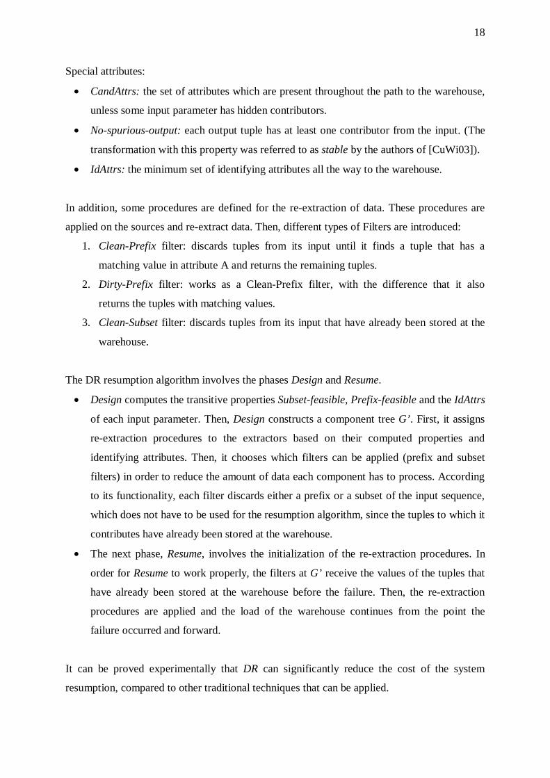
Special attributes:

• CandAttrs: the set of attributes which are present throughout the path to the warehouse,

unless some input parameter has hidden contributors.

• No-spurious-output: each output tuple has at least one contributor from the input. (The

transformation with this property was referred to as stable by the authors of [CuWi03]).

• IdAttrs: the minimum set of identifying attributes all the way to the warehouse.

In addition, some procedures are defined for the re-extraction of data. These procedures are

applied on the sources and re-extract data. Then, different types of Filters are introduced:

1. Clean-Prefix filter: discards tuples from its input until it finds a tuple that has a

matching value in attribute A and returns the remaining tuples.

2. Dirty-Prefix filter: works as a Clean-Prefix filter, with the difference that it also

returns the tuples with matching values.

3. Clean-Subset filter: discards tuples from its input that have already been stored at the

warehouse.

The DR resumption algorithm involves the phases Design and Resume.

• Design computes the transitive properties Subset-feasible, Prefix-feasible and the IdAttrs

of each input parameter. Then, Design constructs a component tree G’. First, it assigns

re-extraction procedures to the extractors based on their computed properties and

identifying attributes. Then, it chooses which filters can be applied (prefix and subset

filters) in order to reduce the amount of data each component has to process. According

to its functionality, each filter discards either a prefix or a subset of the input sequence,

which does not have to be used for the resumption algorithm, since the tuples to which it

contributes have already been stored at the warehouse.

• The next phase, Resume, involves the initialization of the re-extraction procedures. In

order for Resume to work properly, the filters at G’ receive the values of the tuples that

have already been stored at the warehouse before the failure. Then, the re-extraction

procedures are applied and the load of the warehouse continues from the point the

failure occurred and forward.

It can be proved experimentally that DR can significantly reduce the cost of the system

resumption, compared to other traditional techniques that can be applied.

19

2.4. Optimization of Queries with Expensive Predicates

Object – Relational database management systems allow users to define new data types and

new methods for these types. In [Hell98] the author presents a study of optimization

techniques that contain time-consuming methods. These “expensive methods” are natural for

user-defined data types, which are often large objects that contain complex information (e.g.

images, video, maps, fingerprints, etc.).

Traditional query optimizers have focused on “pushdown” rules that apply selections in an

arbitrary order before as many joins as possible. In case any of these selections involves the

invocation of an expensive method, the cost of evaluating the expensive selection may

outweigh the benefit gained by doing the selection before join. This means that the traditional

optimizer cannot produce an optimal plan. The author proposes an algorithm called Predicate

Migration and proves that it produces optimal plans for queries with expensive methods.

Predicate Migration increases query optimization time modestly, since the additional cost

factor is polynomial in the number of operators in a query plan. Furthermore, it has no effect

on the way that the optimizer handles queries without expensive methods – if no expensive

methods are used, the techniques of the algorithm need not be invoked. With modest overhead

in optimization time, Predicate Migration can reduce the execution time of many practical

queries by orders of magnitude.

Predicate Migration can also be applied to expensive “nested subqueries”. Current relational

languages, such as SQL, have long supported expensive predicates in the form of nested

subqueries, whose evaluation is arbitrarily expensive, depending on the complexity and the

size of the subquery. Traditional optimizers convert these subqueries into joins. The problem

that arises is that not all subqueries can be converted into joins. When the computation of the

subquery is necessary for the predicate evaluation, then the predicate should be treated as an

expensive method.

Some important definitions are the following:

• A predicate is a Boolean factor of the query’s WHERE clause.

• Selectivity of a predicate p is the ratio of the cardinality of the output result to the

cardinality of the input (i.e. the ratio of tuples that satisfy the predicate).

20

• A plan tree is a tree whose leaves are scan nodes and whose internal nodes are either

joins or selections.

• A stream in a plan tree is a path from a leaf node to the root.

• A job module is a subset S’ of nodes in a plan, such that all the other plan nodes have

the same constraint relationship (must precede, must follow or unconstrained) with all

the nodes of S’.

• epi: the differential expense of a predicate pi.

• rank: a metric used for the ordering of expensive selection predicates.

rank=(selectivity-1) / differential cost

Then, some cost formulas are defined for computing the expense of a stream of predicates.

The author now uses the following lemma proved by Monma and Sidney ([MoSi79]): The

minimization of the overall cost is achieved by ordering the predicates in ascending order of

the metric rank. Furthermore, swapping the positions of two nodes with equal rank has no

effect on the cost of the plan tree.

The Predicate Migration Algorithm:

Each of the streams in a plan tree is treated individually and the nodes in the streams are

sorted based on their rank. The order of streams I the plan is constrained in two ways: we are

not allowed to reorder join nodes and we must ensure that each stream stays semantically

correct.

The Predicate Migration algorithm uses the Series-Parallel Algorithm Using Parallel Chains

by Monma and Sidney, which is an O(n logn) algorithm that isolates job modules in a stream,

optimizes each job module individually and uses the results to find a total order for the

stream.

The Predicate Migration algorithm is based on the following idea: To optimize a plan tree,

push all predicates down as far as possible, and then repeatedly apply the Series-Parallel

Algorithm Using Parallel Chains to each stream in the tree, until no more progress can be

made.

• The function predicate_migration pushes all predicates down as far as possible. Then,

for each stream in the tree calls series_parallel function.

21

• The function series_parallel traverses the stream top-down, finding modules of the

stream to optimize. Given a module, it calls parallel_chains to order the nodes of the

module optimally.

• The function parallel_chains finds the optimal ordering for the module and introduces

constraints to maintain that ordering as a chain of nodes. Thus, series_parallel uses the

parallel_chains subroutine to convert the stream, from the top down, into a chain.

• The find_groups routine identifies the maximal-sized groups of poorly ordered nodes.

After all groups are formed, the module can be sorted by the rank of each group.

The Predicate Migration algorithm is guaranteed to terminate in polynomial time, producing a

semantically correct, join-order equivalent tree in which each stream is well-ordered.

An advantage of Predicate Migration is that it works not only for left-deep trees but for bushy

trees as well.

User-defined functions and predicates are supported by many relational database management

systems. These predicates are Boolean factors used in the WHERE clause of SQL queries and

can be very expensive since most of them involve substantial CPU and I/O cost. A logical

approach would be to evaluate the expensive predicate after all the joins the query involves,

so that fewer tuples need to be considered during the evaluation. However, if the predicate has

high selectivity, it would be better to evaluate the expensive predicate first, to reduce the cost

of subsequent joins.

In [ChSh99] the authors address this problem and present a number of related algorithms.

They use the quantity rank of a predicate, which is a metric later used to order predicates

properly. This metric is defined using the following equation: rank = c / (1 – s), where c is

the cost-per-tuple and s is the selectivity of the selection or join predicate. The proposed

approach is based on the selection ordering rule, which is valid when all predicates apply on a

relation without any intervening join nodes. According to this rule, the optimal ordering of a

number of predicates is in the order of ascending ranks and is independent of the size of the

participating relations.

22

The first algorithm is the naive optimization algorithm, which uses the notion of tags. The tag

of a plan is the set of user-defined predicates that belong to the plan and have not been

evaluated yet, i.e., the complement of the set of predicates that were evaluated in the plan.

First the dynamic programming algorithm of System R is applied and all possible plans are

produced. Some of them must be stored and retained for the optimizer’s future steps. Two

plans represent the same expression, if they represent the join of the same set of relations and

have the same tag. If the optimizer produces two plans that represent the same expression,

only one of them is kept and the other is pruned. This reduces the number of plans that have

to be stored for future process. Each produced plan p is compared to those previously stored

plans which occupy the same set of relations with p and have the same tag. If p is more

expensive than the stored plans, it is pruned. Otherwise, p is added to the list of stored plans.

The complexity of this algorithm is exponential in the number of user-defined predicates for a

given number of relations in the query.

To improve the complexity of the above algorithm, the authors exploit the use of rank

ordering and arrange predicates in the order of ascending ranks, even if predicates are

separated by join nodes. This is based on the assumption that all join nodes must satisfy

certain properties. Then, we can order all predicates according to their rank. This makes the

optimization algorithm polynomial in the number of user-defined predicates for a given

number of relations.

2.5. Avoiding Sorting and Grouping in Query Processing

The recent work of Wang and Cherniack [WaCh03] recognizes the benefit of detecting

orderings or grouping requirements needed for a more efficient evaluation of queries. This

can prove to be crucial since sorting and grouping operators are amongst the most costly

operations performed during query evaluation. The authors show that existing orderings and

groupings can be exploited to avoid redundant ordering or grouping operators in query

processing.

Another contribution of this paper is a systematic treatment of groupings. Groupings have not

been treated as thoroughly as orderings. While orderings and groupings as related, groupings

behave differently to some extent. The approach of [WaCh03] treats groupings of tuples in a

23

way similar to orderings, since each grouping can be seen as an ordering of tuples, followed

by an application of a grouping function over the items of the same group.

First, the authors discriminate between primary and secondary orderings and groupings. As

primary orderings and groupings the authors refer to the sort and group operators applied first

to the stream tuples. Secondary orderings and groupings are those which hold within each

group determined by a primary ordering or grouping. Then, Wang and Cherniack introduce

order properties, which are primary and secondary orderings and groupings that hold of

physical representations of relations. The order properties refer to way the relation’s tuples are

physically stored. For example, the order property AO →BG of relation R with schema R(A, B)

suggests that the tuples of R are stored first ordered by A and then (within the block of tuples

with the same A value) grouped by B. Order properties can be used to infer ordering and

grouping constraints, thus it is possible to make decisions on how to “push down” sorts and

avoid unnecessary sorting or grouping over multiple attributes.

The authors propose a Plan Refinement Algorithm that accepts a query plan tree as input and

produces as output an equivalent plan that does not contain any unnecessary sort operators.

These sort operators had initially been used to order or group data tuples. A number of axioms

and identities are presented according to which the refinement algorithm applies. More

specifically, these identities are inference rules used to get all orderings and groupings

satisfied by the plan and are necessary for the operation of the refinement algorithm.

The plan refinement algorithm also requires the introduction of four new attributes, which are

associated to each node of the query plan. These are the keys of the node’s inputs, the

functional dependencies that are guaranteed to hold for the node’s inputs, a single required

ordered property that must hold for the node’s inputs in order for the node to work and finally,

a set of order properties that are satisfied by the node’s outputs. The above properties are

referred to as keys, fds, req and sat respectively and are computed during the execution of the

refinement algorithm.

The algorithm involves three passes of the query plan. The first pass is performed in the

bottom – up direction of the query plan tree and starting from the leaf nodes, keys and

functional dependencies (fds) are computed and propagated upwards through most nodes

24

unchanged, except few operators such as joins, where new keys and functional dependencies

are added, or other operators where keys and dependencies are lost. When these properties are

computed, they decorate the nodes of the query plan. During the second pass, the algorithm

starts at the root of the tree and continues downwards. The required order properties (req) are

calculated according to query operators and inherited from parent nodes to child nodes. The

final pass is a bottom – up pass of the query plan that decides which order properties are

satisfied by each node’s outputs (sat). Then, it removes a node’s subsequent sort operator, if it

has one of these order properties as its required property. This property can be satisfied

without ordering, which means that this sort operator is redundant.

Experiments were held in Postgres and the results showed significant reduction in the plan’s

cost. They showed that when we avoid sorting towards the end of the computation on

intermediate join results where the join selectivity is very low, the plan refinement can reduce

execution costs by an order of magnitude. In addition, further experiments showed that in

most cases the overhead of the plan refinement algorithm added to the query optimization cost

is low.

2.6. Grouping and Order Optimization

In the work of Neumann and Moerkotte ([NeMo04]), the authors recognize the performance-

critical role of interesting orders to the query optimization. First, they differentiate between

physical and logical orderings of a stream of tuples.

- A physical ordering of a set of tuples is an ordering relative to the actual succession of

tuples in the stream.

- On the other hand, logical orderings specify conditions a tuple stream must meet to

satisfy a given ordering.

One form of logical orderings are considered to be interesting orders. Interesting orders are

defined as orderings required by operators of the physical algebra and orderings produced by

such operators. Interesting groupings are defined similarly as groupings required by operators

of the physical algebra and groupings produced by these operators.

25

The authors suggest that functional dependencies can be used to infer new orderings and new

groupings. It is assumed that relevant functional dependences are known, since they can be

discovered with the procedure described in detail in [SiSM96]. Thus, Neumann and

Moerkotte define an inference mechanism based on the following ideas:

1. Given a logical ordering o = (Ao1, …, Aom) of a tuple stream R, then R obviously

satisfies any logical ordering that is a prefix of o including o itself.

2. Given two groupings g and g’ ⊂ g and a tuple stream R satisfying the grouping g, R

need not satisfy the grouping g’.

Based on the above propositions, the authors suggest the construction of a finite state machine

(FSM) to represent the set of logical orderings. The states of the FSM represent physical

orderings and the edges are labeled with functional dependencies. Since one physical ordering

can imply multiple logical orderings, є-edges are used. As a result, the FSM is Non-

deterministic. Before the actual plan generation the Non-deterministic FSM (NFSM) is

converted into a Deterministic FSM (DFSM). The FSM allows order optimization operations

in O(1) time. Furthermore, the authors suggest constructing a similar FSM for groupings and

integrating it into the FSM for orderings. The FSM for groupings is similar to those for

orderings but much smaller, since groupings are only compatible with themselves, no nodes

for prefixes are required. The FSM for groupings is integrated into the FSM for orderings by

adding є-edges from each ordering to the grouping with the same attributes. This is due to the

fact that each ordering is also a grouping. Moreover, pruning techniques are used to minimize

the size of the NFSM. This NFSM must be converted into a DFSM.

Experimental results show that with a modest increase of the time and space requirements

both orderings and groupings can be handled at the same time. More importantly, there is no

additional cost for the addition of groupings in the order optimization framework.

2.7. Comparison of our Work to Related Work

So far, research work has not dealt with the problem of mapping a logical ETL scenario to

alternative physical ones. Most papers are concerned with query optimization techniques.

These papers focus on queries and do not handle ETL processes. ETL processes cannot be

26

treated as “big” queries, since they contain activities which run in separate environments,

usually not simultaneously and under time constraints. Thus, the traditional techniques for

query optimization can not be applied, due to data-manipulation functions with unknown or

impossible to express semantics.

For the moment, research approaches have focused on topics, such as the order optimization,

which refers to the subarea of plan generation that is concerned with handling interesting

orders. This problem is one of the issues an optimizer has to address during the evaluation of

queries. Part of the optimizer’s job is to produce one or more interesting orders, i.e., a set of

ordering specifications that can be useful for the query rewriting and the generation of a plan

with lower cost. The first paper to address this problem was the paper of P. Selinger et al

[SAC+79] that dealt with query optimization techniques. Later papers ([SiSM96], [Hell98],

[WaCh03]) have mainly focused on techniques to “push down”, or combine existing orders in

query plans.

Furthermore, many of the studies employ interesting orders, but rely on functional

dependencies ([SiSM96], [NeMo04]) and predicates applied over data, without handling

orders more abstractly. Existing work is concerned with the exploitation of orderings, for

optimization purposes, although the introduction of new orderings is not considered at all.

In their work, Wang and Cherniack ([WaCh03]) recognize that orderings and groupings are

expensive operations and propose the pruning of redundant orderings and groupings. The

proposed Plan Refinement Algorithm produces an equivalent query plan without unnecessary

order or group operators. Thus, the authors manipulate existing orderings and groupings and

do not explore the possibility of adding orderings to a given workflow, or the benefits of this

procedure.

In the work of [NeMo04] and [WaCh03], the authors recognize the performance-critical role

of interesting orders to the query optimization. Their research work proposes the exploitation

of orderings and groupings in query plans. They focus on the utilization of functional

dependencies and propose a set of inference rules for the deduction of logical orderings.

27

On the other hand, the authors of [SiVS05] deal with ETL workflows and their optimization

and propose a set of transitions that generate equivalent workflows possibly with lower cost.

In this work, interesting orders are not considered.

Hellerstein [Hell98] deals with left-deep or bushy relational query plans and not ETL

workflows. Thus, we can not employ the procedures or the cost model proposed by

Hellerstein.

In the research work of Labio et al ([LWGG00]), the authors present a resumption technique

that can be initiated in case of failures to resume a failed load. On the other hand, the authors

of [CuWi03] are considered with a different problem: they handle the data lineage problem,

which means tracing certain warehouse data items back to the original source items from

which they were derived.

28

CHAPTER 3. FORMAL STATEMENT OF THE

PROBLEM

3.1 Formal Statement of the Problem

3.2 Introduction of Sorter Activities to an ETL Workflow

3.3 Reference Example

3.4 System Failures - Resumption

In this section, we first describe the structure of an ETL workflow. Then, we discuss the

generic properties of activities and logical-to physical mappings. We also present a library of

templates for activities and model the problem as a state-space search problem. Then, we

present the formal definition of the problem addressed in this thesis. Furthermore, we present

a library of transformations. Then, we discuss the exploitation of orderings in minimizing the

cost of the physical implementation of ETL scenarios. For this reason, we introduce a special-

purpose set of activities, which we refer to as Sorters and present their characteristics.

3.1. Formal Statement of the Problem

3.1.1. The Structure of an ETL Workflow

An ETL workflow captures the flow of data from the sources to the data warehouse and/or

data marts. In this work, we model an ETL workflow as a directed acyclic graph (DAG)

G(V,E), where V is the set of the graph nodes and E the set of edges which connect the nodes.

Each node v ∈ V is either an activity or a recordset.

• An activity is a software module that processes the incoming data, either by

performing some transformations over the data or by applying data cleansing

29

procedures. Activities have one or more input schemata, i.e., finite lists of attributes

that describe the schema of the data coming from the data providers of the activity. An

activity with one input schema is called unary, while an activity with two input

schemata is called binary. Activities also have one or more output schemata which

play the role of the schemata that provide the processed data to the subsequent nodes.

Furthermore, the semantics of the activity is an expression in an extended relational

algebra with black-box functions that characterizes the activity.

• A recordset is a set of records in the form of a data storage structure. Formally, a

recordset is characterized by its name, its logical schema and its physical extension

(i.e., a finite set of records under the recordset schema). Recordsets have exactly one

schema that describes the structure of the stored data. If we consider a schema

S=[A1,…,Ak], for a certain recordset, where Ai , i=1,…,k are schema attributes, its

extension is a mapping S=[A1,…,Ak]→dom(A1)×…×dom(Ak). Thus, the extension of

the recordset is a finite subset of dom(A1)×…×dom(Ak) and a record is the instance of

a mapping dom(A1)×…×dom(Ak)→[x1,…,xk], xi∈dom(Ai). Thus, a record is defined as

the instantiation of a schema to a list of values belonging to the domains of the

respective schema attributes. In the rest of this work, we will mainly deal with the two

most popular kinds of recordsets, i.e., relational tables and record files. Relational

tables consist of structured data (i.e., data having an internal structure that follows a

specific schema), whereas data stored in files can be unstructured (where data cannot

be constrained within a schema such as image, video or audio files) or semi-structured

(such as web content where there is no separate schema for the data or a schema exists

but places loose constraints over data). For the latter case, we assume the existence of

a relational wrapper that abstracts the physical details under a relational, logical

schema.

To fully capture the characteristics and interactions of the activities and recordsets mentioned

previously, we model their relationships as the edges of the graph. The edges of the graph

denote data provider relationships. An edge (a, b) coming out of a node a into a node b

denotes that b receives data from node a for further processing. Node a plays the role of the

data provider, while node b is the data consumer. In our setting, we allow recordsets to have

more than one data consumers. On the other hand, we limit our consideration to activities with

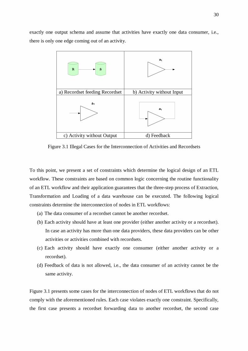
30

exactly one output schema and assume that activities have exactly one data consumer, i.e.,

there is only one edge coming out of an activity.

Figure 3.1 Illegal Cases for the Interconnection of Activities and Recordsets

To this point, we present a set of constraints which determine the logical design of an ETL

workflow. These constraints are based on common logic concerning the routine functionality

of an ETL workflow and their application guarantees that the three-step process of Extraction,

Transformation and Loading of a data warehouse can be executed. The following logical

constraints determine the interconnection of nodes in ETL workflows:

(a) The data consumer of a recordset cannot be another recordset.

(b) Each activity should have at least one provider (either another activity or a recordset).

In case an activity has more than one data providers, these data providers can be other

activities or activities combined with recordsets.

(c) Each activity should have exactly one consumer (either another activity or a

recordset).

(d) Feedback of data is not allowed, i.e., the data consumer of an activity cannot be the

same activity.

Figure 3.1 presents some cases for the interconnection of nodes of ETL workflows that do not

comply with the aforementioned rules. Each case violates exactly one constraint. Specifically,

the first case presents a recordset forwarding data to another recordset, the second case

a) Recordset feeding Recordset b) Activity without Input

c) Activity without Output d) Feedback

31

involves an activity that has no input, while the third case shows an activity with no output.

Finally, the fourth case contains feedback of data.

3.1.2. Generic Properties of Activities

Each activity has a number of properties that describe its functionality as a constituent of an

ETL workflow. We now present the generic properties of activities:

1. Each activity is characterized by a name (a unique identifier for the activity).

2. Each activity can have one input schema (unary) or two input schemata (binary).

3. Each activity has exactly one output schema.

4. In order for the activity to be executed, its input data must satisfy one or more

conditions. From this point, we will refer to such conditions as preconditions for the

activity’s execution.

5. There exist one or more different implementation algorithms for the activity’s

execution.

6. The activity produces output data that satisfy some ordering or not.

7. It is possible that one or both its inputs have to be stored.

8. Type/Class of the activity. Different kinds of activities have different characteristics

and different time and system requirements. Thus, they produce different

computational costs.

9. Selectivity of an activity is a numeric value that describes the percentage of input

tuples that appear in the output. It is computed as the ratio of the cardinality of the

output to the cardinality of the input.

10. Each activity is characterized by its semantics, i.e., a description of its functionality

expressed in a program in a declarative database language (e.g., SQL, Datalog, etc.)

extended with black-box functions.

3.1.3. Logical to Physical Mappings

We now define some terms that are useful to our approach. First, we discuss the difference

between the logical-level activity and the physical-level activity.

32

- A logical-level activity is a representation of the activity that describes declaratively

the relationship of the output with the input without delving into algorithmical or

implementation issues. For example, the notation R><S is a logical-level join of tables

R and S and does not provide further information on the implementation technique

followed for the activity’s execution.

- A physical-level activity is a representation of the activity that includes detailed

information on the implementation techniques that must be employed for the activity’s

execution. For example, assume an activity a1 which performs the join of tables R and

S. If we define that this join is implemented using the Nested-Loops algorithm, the

execution engine is informed about the inner procedures followed to produce the result

of the join and can be aware of the cost of this implementation in terms of time or

system resources like memory, disk space allocation, etc.

Mapping of a Logical-Level Activity to Alternative Physical-Level Activities

Pretty much like in traditional query processing, each logical-level activity of an ETL

workflow can be implemented physically using a number of different methods. We represent

each of these implementation methods using a physical-level activity, as defined in the

previous paragraph. In this setting, we can assume a one-to-many mapping (i.e., 1:N

relationship) between the logical-level and the physical-level activities as follows: one

logical-level activity can possibly have more than one physical implementations while a

physical implementation of an activity can only correspond to one logical-level activity).

Figure 3.2 presents the example of an ETL scenario that consists of two sources R and S, a

join activity a1 and a target data warehouse DW. In this scenario, the logical-level activity a1

can be implemented physically using one of the following algorithms: Nested-Loops Join,

Merge Join, Sort-Merge Join or Hash Join. Figure 3.3 presents the mapping of a logical-level

join to a set of alternative physical implementations.

A physical-level implementation for an activity is characterized by the following elements:

• The algorithm employed for the physical execution of the activity,

• A set of constraints that determine whether this physical implementation is feasible or

not. Certain physical implementations can be implemented only if specific conditions

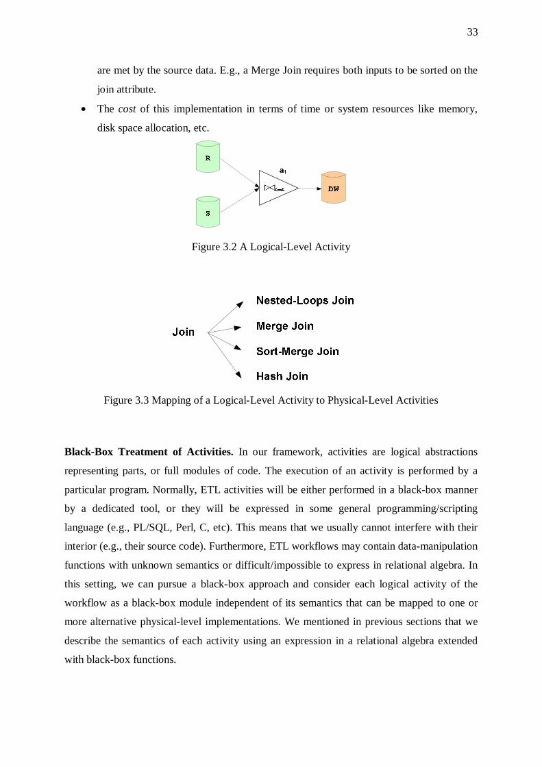
33

are met by the source data. E.g., a Merge Join requires both inputs to be sorted on the

join attribute.

• The cost of this implementation in terms of time or system resources like memory,

disk space allocation, etc.

Figure 3.2 A Logical-Level Activity

Figure 3.3 Mapping of a Logical-Level Activity to Physical-Level Activities

Black-Box Treatment of Activities. In our framework, activities are logical abstractions

representing parts, or full modules of code. The execution of an activity is performed by a

particular program. Normally, ETL activities will be either performed in a black-box manner

by a dedicated tool, or they will be expressed in some general programming/scripting

language (e.g., PL/SQL, Perl, C, etc). This means that we usually cannot interfere with their

interior (e.g., their source code). Furthermore, ETL workflows may contain data-manipulation

functions with unknown semantics or difficult/impossible to express in relational algebra. In

this setting, we can pursue a black-box approach and consider each logical activity of the

workflow as a black-box module independent of its semantics that can be mapped to one or

more alternative physical-level implementations. We mentioned in previous sections that we

describe the semantics of each activity using an expression in a relational algebra extended

with black-box functions.

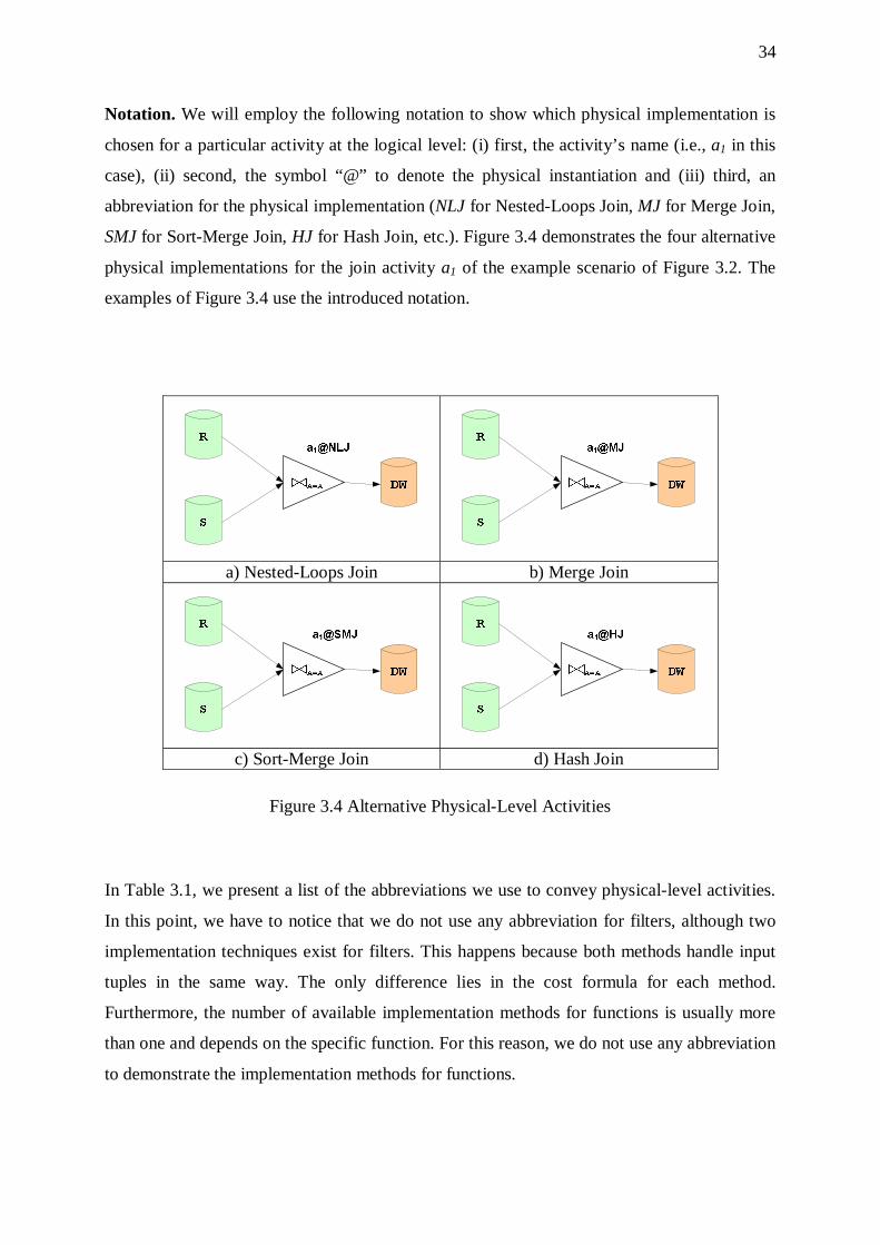
34

Notation. We will employ the following notation to show which physical implementation is

chosen for a particular activity at the logical level: (i) first, the activity’s name (i.e., a1 in this

case), (ii) second, the symbol “@” to denote the physical instantiation and (iii) third, an

abbreviation for the physical implementation (NLJ for Nested-Loops Join, MJ for Merge Join,

SMJ for Sort-Merge Join, HJ for Hash Join, etc.). Figure 3.4 demonstrates the four alternative

physical implementations for the join activity a1 of the example scenario of Figure 3.2. The

examples of Figure 3.4 use the introduced notation.

Figure 3.4 Alternative Physical-Level Activities

In Table 3.1, we present a list of the abbreviations we use to convey physical-level activities.

In this point, we have to notice that we do not use any abbreviation for filters, although two

implementation techniques exist for filters. This happens because both methods handle input

tuples in the same way. The only difference lies in the cost formula for each method.

Furthermore, the number of available implementation methods for functions is usually more

than one and depends on the specific function. For this reason, we do not use any abbreviation

to demonstrate the implementation methods for functions.

a) Nested-Loops Join b) Merge Join

c) Sort-Merge Join d) Hash Join

35

Table 3.1 Abbreviations for Physical-Level Activities

Logical-Level Activity Physical-Level Activities Abbreviation Filter – – Join Nested-Loops Join

Merge-Join Sort-Merge Join

Hash Join

NLJ MJ

SMJ HJ

Aggregation Nested-Loops Sort-based Hash-based

NL SO HS

Function – –

Templates. To facilitate the mapping of a logical-level activity to its alternative physical-

level implementations, we can build an ETL engine using templates for activities and

customizing them per scenario. Therefore, in the rest of this work we will provide a library of

templates for ETL activities. Each template in this library has a set of properties, which

involve some predefined semantics and a set of parameters that determine the functionality of

the template. To construct a certain activity, the designer continues to the instantiation phase:

the designer picks a certain template from the library of templates and specifies the input

schemata and the output schema of the activity and provides concrete values to the template

parameters.

For example, when the designer of a workflow materializes a Not_Null template he must

specify the attribute over which the check is performed. Then, these parameters are replaced

by the concrete values defined by the designer.

In this work, we employ two categories of templates:

1. logical templates that materialize logical-level activities and

2. physical templates that materialize physical-level activities.

We assume a library of logical templates and a library of physical templates. Similar to

logical and physical activities, there is a 1:N mapping between logical and physical templates.

Using logical and physical templates, a certain physical-level activity is constructed as

follows:

• the designer picks a logical template out of the library of logical templates

36

• in order to create the logical instance of the activity he specifies necessary schemata

and concrete values for the logical template parameters

• the logical-to-physical mapping of templates produces one or more physical templates

• if certain constraints/preconditions are met, the physical template is instantiated to a

physical instance.

To elucidate the above consideration, we present the generic properties of templates and

instances in Table 3.2.

Table 3.2 Properties of Templates / Instances

LOGICAL TEMPLATE LOGICAL INSTANCE 1. A finite set of input schemata 2. An output schema 3. Semantics (abstract) 4. A set of physical template

implementations

1. Name 2. Belongs to a logical template,

whose schemata it customizes with specific attributes

3. Semantics (concrete) PHYSICAL TEMPLATE PHYSICAL INSTANCE

1. A logical template to which it refers 2. Preconditions concerning:

a. storage of input b. ordering of input

3. Output order 4. Cost formula 5. Implementation Algorithm

1. Cost

We illustrate the logical-to-physical mappings of activities using templates with the example

of a Filter σΒ>500. We present the templates and instances for this Filter in Table 3.3.

Summarizing, the procedure to construct a physical-level activity is the following:

a. Based on the logical-level activity, find the logical template for the activity.

b. Map the logical template to one or more physical templates.

c. Taking into consideration all physical-level constraints, customize each physical

template to a physical-level activity.

37

Table 3.3 Properties Templates / Instances for a Filter

LOGICAL TEMPLATE LOGICAL INSTANCE 1. Input schema: (#1, #2, …, #N) 2. Output schema: (#1, #2, …, #N) 3. Semantics (abstract): σ$1op $2 4. A set of physical template

implementations

1. Name: a1 2. Belongs to the logical template of

Filters 3. Input schema: (A, B, C) 4. Output schema: (A, B, C) 5. Semantics (concrete): σΒ>500

PHYSICAL TEMPLATE PHYSICAL INSTANCE 1. It refers to the logical template for

Filters 2. No Preconditions 3. Output order: Same as Input Order 4. Cost formula: 5. Cost(σ) = selectivity(σ)* |input

tuples| 6. Implementation Algorithm

1. Cost = 1000

Mapping of a Logical-Level Scenario to Alternative Physical-Level Scenarios

Having discussed the mapping of a logical-level activity to its physical implementations, we

continue our consideration to the scenario-level. Similarly, we define the logical-level

scenario as opposed to the physical-level scenario.

• A logical-level scenario is a representation of the scenario that identifies it as a

collection of data stores and activities that extract data from the sources, process it and

propagate it further to the data warehouse and/or data marts. This description of the

scenario does not delve into algorithmical or implementation issues.

• A physical-level scenario is a description of the scenario that states declaratively the

implementation methods that have to be followed for the physical execution of the

scenario. Obviously, the physical-level scenario consists of physical-level activities.

The obvious question that arises in this setting is the following: Given a logical-level scenario

and a set of templates for logical activities, how can we discover all the corresponding

physical-level scenarios?

The procedure to determine the alternative physical-level scenarios is presented next:

• First, identify the appropriate logical template of each activity of the workflow.

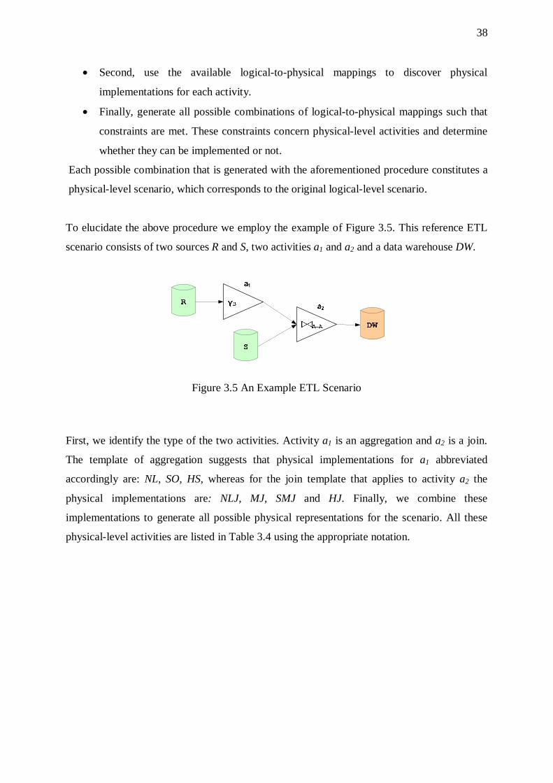
38

• Second, use the available logical-to-physical mappings to discover physical

implementations for each activity.

• Finally, generate all possible combinations of logical-to-physical mappings such that

constraints are met. These constraints concern physical-level activities and determine

whether they can be implemented or not.

Each possible combination that is generated with the aforementioned procedure constitutes a

physical-level scenario, which corresponds to the original logical-level scenario.

To elucidate the above procedure we employ the example of Figure 3.5. This reference ETL

scenario consists of two sources R and S, two activities a1 and a2 and a data warehouse DW.

Figure 3.5 An Example ETL Scenario

First, we identify the type of the two activities. Activity a1 is an aggregation and a2 is a join.

The template of aggregation suggests that physical implementations for a1 abbreviated

accordingly are: NL, SO, HS, whereas for the join template that applies to activity a2 the

physical implementations are: NLJ, MJ, SMJ and HJ. Finally, we combine these

implementations to generate all possible physical representations for the scenario. All these

physical-level activities are listed in Table 3.4 using the appropriate notation.

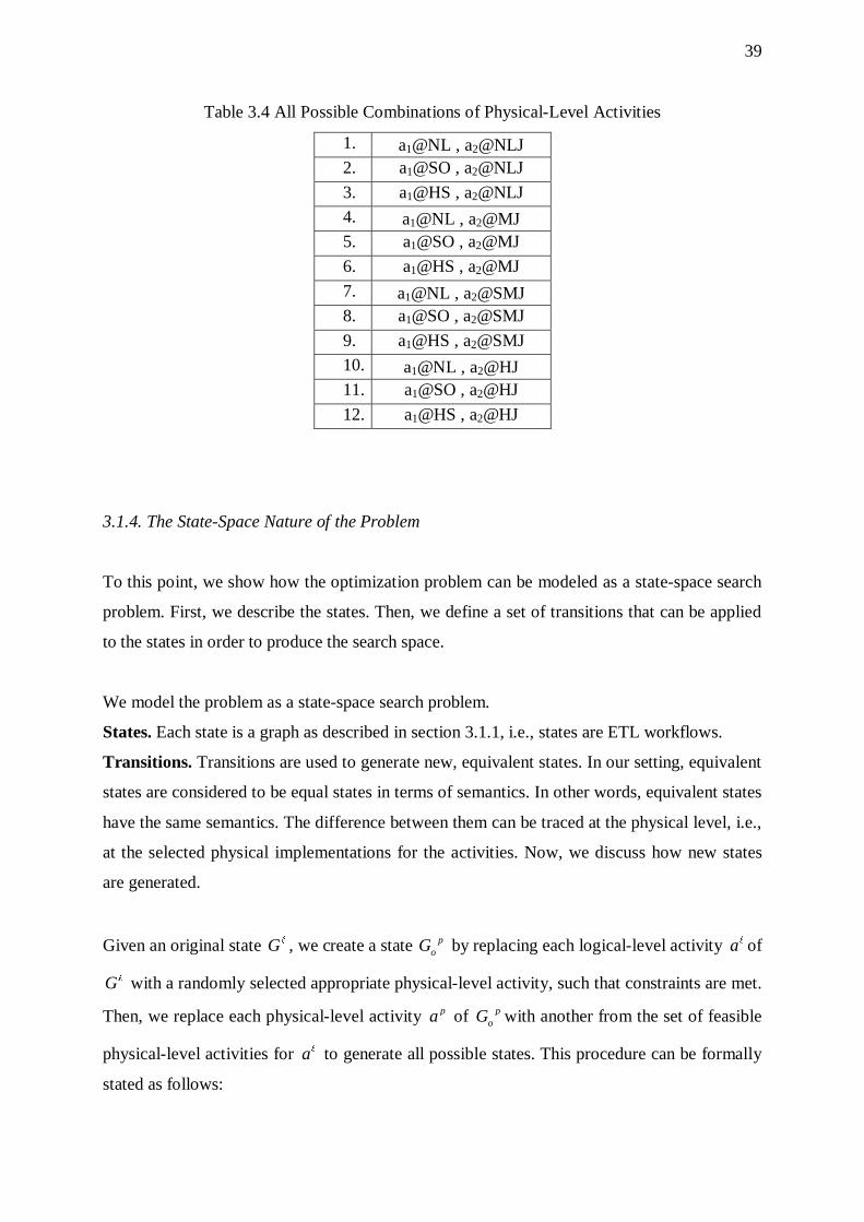
39

Table 3.4 All Possible Combinations of Physical-Level Activities

3.1.4. The State-Space Nature of the Problem

To this point, we show how the optimization problem can be modeled as a state-space search

problem. First, we describe the states. Then, we define a set of transitions that can be applied

to the states in order to produce the search space.

We model the problem as a state-space search problem.

States. Each state is a graph as described in section 3.1.1, i.e., states are ETL workflows.

Transitions. Transitions are used to generate new, equivalent states. In our setting, equivalent

states are considered to be equal states in terms of semantics. In other words, equivalent states

have the same semantics. The difference between them can be traced at the physical level, i.e.,

at the selected physical implementations for the activities. Now, we discuss how new states

are generated.

Given an original state Gl , we create a state poG by replacing each logical-level activity al of

Gl with a randomly selected appropriate physical-level activity, such that constraints are met.

Then, we replace each physical-level activity pa of poG with another from the set of feasible

physical-level activities for al to generate all possible states. This procedure can be formally

stated as follows:

1. a1@NL , a2@NLJ 2. a1@SO , a2@NLJ

3. a1@HS , a2@NLJ

4. a1@NL , a2@MJ 5. a1@SO , a2@MJ

6. a1@HS , a2@MJ

7. a1@NL , a2@SMJ 8. a1@SO , a2@SMJ

9. a1@HS , a2@SMJ

10. a1@NL , a2@HJ 11. a1@SO , a2@HJ

12. a1@HS , a2@HJ

40

Given a logical graph ( , )G V El l l , then determine the physical-level graph ( , )p p po o oG V E , as

follows: , p poa V a V∀ ∈ ∃ ∈l l , where al is a logical-level activity, while pa is a physical-

level activity. Then, p poa V∀ ∈ replace pa with 'pa such that ', _ ( )p pa a phys impl a∈ l , where

phys_impl(i) is the set of feasible physical implementations of activity i.

We assume a given logical-level ETL scenario and a set of physical-level scenarios generated

with the procedure discussed in the previous section. We have already mentioned that each

physical-level activity has different cost, i.e., requirements in terms of system resources or

time specifications. In this setting, it is not obvious which of the generated physical-level

scenarios is best in terms of performance gains. In order to choose the optimal scenario at

physical level, we have to introduce a cost model or the estimation of the cost of each activity.

Based on the cost model, the cost of each generated physical-level scenario is computed and

the one with minimal cost is selected.

Now, we can review the problem we have to address, which has various sides:

• First, establish a cost model suitable for our system. According to the cost model, we

can specify the cost of the workflow activities.

• Second, given a logical representation of an ETL scenario, determine all physical-level

implementations of the scenario.

• Finally, determine the optimal configuration with respect to its performance, out of the

collection of physical-level scenarios.

3.1.5. Formal Definition of the Problem

Assume a library of logical template activities 1 2, ,..., nL t t t=l l l l . Also assume a library of

physical template activities 1 2, ,...,p p p pzL t t t= and a 1:N mapping among them 2:

p

m L L→l .

The mapping m maps each logical template to a set of physical template implementations.

Assume an infinitely countable set A of activities and an infinitely countable set Ω of

templates. Assume a transformation T, such that: T : A Ω.

41

Assume an activity a which is a materialization of template t. We denote this fact through the

function T that maps an activity a to its appropriate template t. In our case, T(a) = t. The

function T applies both to logical and physical-level activities.

Assume also the mapping CG(V,E), which is the inverse of function T. Then, CG(V,E) : Ω A.

Given a logical scenario G(V,E), the customization of a template t for an activity a belonging

to V is given by the mapping CG(V,E)(t)= a.

Assume a physical-level activity a. Then constr(a) is a predicate in a simple conjunctive form

denoting the set of constraints that exist for the physical implementation of activity a. I.e.,

constr(a) = 1 2 ... kc c c∧ ∧ ∧ , where ci =1,…, k are constraints.

Assume an activity a. Then, cost(a) is a function that returns the cost of an activity. The cost

of an activity depends on the cost model and possibly on its position on the workflow.

Furthermore, the cost of the activity depends on the physical implementation that is selected

for its execution. Then, the total cost of the scenario is obtained by summarizing the cost of all

its activities. In other words, the total cost of the scenario is given by the following formula:

Cost(G) =1

( )n

icost i

=∑ , where n is the number of the activities of the scenario.

Having introduced all necessary definitions concerning templates, mappings and available

functions, we can now present the formal definition of the problem, which can be stated as

follows:

Given a logical-level graph ( , )G V El l l , where 1 2 1 2, ,..., , , ,...,n kV a a a r r r=l l l l and

,ia i 1,...,n=l are logical-level activities, ,ir i 1,...,k= are recordsets, then determine the

physical-level graph ( , )p p pG V E , with 1 2 1 2, ,..., , , ,...,p p p pn kV a a a r r r= , where ,p

ia i 1,...,n=

are physical-level activities, such that:

• ( )( )( )( , )

pi iG V E

a C m T a∈ l l l

l , i=1,…,n

• ( , ),i je a a e E∀ = ∈l l l l l , introduce pe to pE where ( , )p p pi je a a=

• ( , ),i je a r e E∀ = ∈l l l l , jr V∈ l introduce pe to pE where ( , )p pi je a r=

42

• ( , ),i je r a e E∀ = ∈l l l l , ir V∈ l introduce pe to pE where ( , )p pi je r a=

• ( )i

piconstr a trueΛ = , i=1,…,n

• ( )i

p

icost a∑ = minimal, i=1,…,n

The above problem formulation states that in order to construct a physical-level activity, the

procedure is the following:

a. Apply function T on the logical-level activity to find the logical template for the

activity.

b. Map the logical template to one or more physical templates (using mapping m).

c. Customize each physical template to a physical-level activity.

If we perform this procedure for each logical activity of the workflow, taking into

consideration all physical-level constraints, we construct a physical-level scenario. The

physical scenario having minimal cost is the optimal scenario.

3.1.6. Issues Concerning the State-Space Nature of the Problem Formulation

An obvious issue that arises in our setting concerns this mapping of a given logical

description of an ETL scenario to all the available physical ones. We come across to the

following questions:

1. Which mappings are legal for our activities?

2. Which physical-level description of the scenario is the best in terms of performance

gains?

In the following paragraphs we will refer to each of the above considerations separately.

Legal Mappings for activities. We also have to mention that some of the mappings may

produce physical-level scenarios that can not be feasible, since certain physical

implementations of activities require some preconditions to be fulfilled in order to be

executed. Examples of such preconditions for activities are discussed in detail in section 3.1.7

where we present a library of templates for logical activities and their characteristics. For the

moment, we simply mention two examples of such:

• Both inputs of a merge-join template have to be ordered according to the join attribute.

43

• The second input of a join template must be stored.

Discover Physical-Level Scenario having Minimal Cost. Having outlined the state-space

generation, we now move on to make a few general remarks concerning the cost model and

the identification of the configuration with the minimum cost.

In order to choose the optimal physical representation, we have to introduce a discrimination

criterion among physical-level ETL scenarios. This criterion is a cost model, used for the

estimation of the cost of each activity. The selection of a cost model is a difficult task in our

case, because of the existence of black-box activities and functions. In the work of Hellerstein

([Hell98]), the author states that black-box activities can be written in a general programming

language such as C, or in a database query language, for example, SQL. Given that black-box

functions may be written in a general-purpose language such as C, Hellerstein recognizes that

it is difficult to correctly estimate the cost of these functions, at least initially. The only

available information is the initial size of input data. After repeated applications of a black-

box function, one could collect performance statistics, such as the average Cost_per_tuple of

each black-box activity, the output size as a function of the input size, etc. Then, using curve-

fitting techniques (e.g., interpolation) one can make estimates about the activity’s behavior.

On the other hand, it can be difficult to estimate the cost of an activity written in a procedural

language, because of the non-declarative statements that this activity may contain. For

example, for cases of various if/for/while statements, the execution time (and consequently

the total cost and the Cost_per_tuple) for the activity depend on undefinable factors. Based on

the above considerations, we can say that a cost model useful for our case should be able to

incorporate black-box activities with unknown semantics. On the other hand, if the internals

of such an activity is known (white-box semantics), we should be able to plug-in more

elaborate formulae to the cost model.

Hellerstein uses the principle of optimality proposed by Monma and Sidney ([MoSi79]),

which states that the cost of a set of predicates can be minimized by rearranging them in

ascending order of the metric rank. The problem that appears in our setting is that this

principle of optimality does not work for our case, because we do not deal with left-deep or

bushy relational query plans, but ETL workflows. Thus, we can not employ the cost model

proposed by Hellerstein. Furthermore, the formulae for the cost model of Hellerstein assume

44

that the cost of passing parameters to functions is known. This is impossible for black-box

functions.

We now refer to a set of properties that the chosen cost model should have:

1. First, the cost model must be generic enough to apply to the black-box abstraction of

activities.

2. Second, the model should provide the means to evaluate the performance of the

proposed algorithm, in terms of time or system requirements.

3. It should take into consideration the possibility of failures during the warehouse load

and it should provide formulae that calculate the expected cost of resuming load after

the system recovery.

Now, we can proceed to the identification of the configuration having minimum cost. The

obvious, exhaustive procedure is the following:

• Based on the chosen cost model, we compute the cost of each physical description of

the scenario.

• Then, we compare the costs of the physical descriptions and select the one having the

minimum cost.

3.1.7. Library of Transformations

To exemplify how the aforementioned generic properties of activities fit with our framework,

we discuss the following four broad categories of activities: Filters (σ), Joins (><),

Aggregations (γ) and Function applications (f). In this section, we describe in detail these four

categories of transformations and their characteristic properties:

1. Filters (σφ(R)):

• Filters are unary activities that provide checks for the satisfaction (or not) of a certain

condition. The semantics of these filters are the obvious (starting from a generic

selection condition φ and proceeding to the check for null values, primary or foreign

key violation, etc.). Filters preserve the schema of the input to the output.

• No precondition has to be fulfilled in order for the filter to be executed.

45

• There are two different physical implementations for filters. Assume a relation R:

a. The obvious, exhaustive method to implement a filter is to scan the entire

relation R and perform the check on each tuple, outputting those that satisfy it.

This leads to the following formula for the filter’s cost:

Cost(σ(R)) = |input tuples|

If only a small number of tuples satisfy the condition, the cost of scanning the

entire relation is high.

b. In case a filter receives tuples ordered according to the attribute that

participates in the selection condition φ, we avoid the complete scan of the

input tuples and examine only the first selectivity(σ(R))* |input tuples| tuples.

The cost of the filter now becomes:

Cost(σ(R)) = selectivity(σ(R))* |input tuples|

• Filters retain the order of their input data to their output data.

• The filter’s input does not have to be stored.

2. Joins (R >< R.A=S.A S):

• Joins are binary activities.

• The necessary precondition for all join algorithms is that the inner input has to be

stored. For example, for the join R><S, S must be stored. Furthermore, a specific

precondition exists for the Merge-Join template: both inputs have to be sorted on the

join attribute.

• A join can be evaluated using one of the following algorithms:

o Nested-Loops algorithm: For each tuple in the outer join relation, the entire

inner join relation is scanned, and any tuples that match the join condition are

added to the result set. Naturally, this algorithm performs poorly if either the

inner or outer join relation is very large.

o Merge Join: It requires that both relations R and S are sorted on the join

attribute. Then, it merges the two relations by matching only tuples that have

the same value in the join attribute.

o Sort-Merge Join: It is another way to evaluate a join and resembles Merge-

Join. The only difference is that Sort-Merge-Join first sorts each relation on the

join attribute and then finds matching tuples using a merge procedure: it scans

46

both relations simultaneously and compares the join attributes. When a match

is found, the joined tuple is added to the result.

o Hash Join: Applying the hash join algorithm on a join of two relations

proceeds as follows: Assuming that the smaller relation fits in main memory,

we prepare a hash table for the smaller relation, by applying a hash function to

the join attribute of each tuple, and then we scan the larger relation and find the

matching tuples by looking on the hash table.

• According to the different implementations, output data can be ordered or not. We will

discuss each implementation separately:

o Nested-Loops: The ordering of output data is the same as the ordering of the

data coming from the outer relation of the join.

o Merge Join: Output data are ordered according to the join attribute.

o Sort-Merge Join: Output data are ordered according to the join attribute.

o Hash Join: Output data do not have an ordering.

• The cost of the join depends on the implementation: if n = |input tuples of R| and m =

|input tuples of S|, then:

o Nested-Loops Join(NLJ):

Cost(γNLJ(R)) = n+(n/ √(b)) * m , where b=max(n, m)

o Merge Join(MJ):

Cost(γMJ(R)) = n+m

o Sort-Merge Join(SMJ):

a. The cost of SMJ is:

Cost(γSMJ(R)) = n*log2n+m*log2m+n+m

b. The Sort-Merge Join can be computed less costly if both inputs are ordered

according to the values of the join attribute. Then, there is no need to order

the inputs, so the cost of Sort-Merge Join becomes equal to the cost of

Merge Join:

Cost(γSMJ(R)) = n+m

o Hash Join(HJ):

Cost(γHJ(R)) = 3*(n+m)

To the above formulae, if the inputs of the join are not stored, we add the cost (n+m) to store

it and read it afterwards.

47

3. Aggregations (γ grouping-list(R)):

• Aggregations are unary activities used to condense information about large volumes of

data. Aggregation is based on the idea of partitioning items into groups and

representing each group with a single value. The grouping-list consists of a number of

attributes that participate in the partitioning. Data is divided into groups according to

the values of the grouping attributes.

• An Aggregation can be evaluated using one of the following algorithms:

o Nested-Loops: a temporary file is used to aggregate output data. For each input

record, the algorithm searches the output file to find it. If the search is

successful, the output file is updated to include the input data. Otherwise, a

new group is created to the output file to include the incoming record.

o Sort-based implementation: Data are first ordered according to the grouping

attributes. This way similar tuples are placed in neighboring positions and

afterwards each tuple is placed into the appropriate group. This implementation

of aggregations can exploit any preexisting ordering of the input data, since in

case such an ordering exists we do not have to sort the initial data to perform

the grouping.

o Hash-based implementation: With hashing, we hash on the aggregation key.

Then tuples that belong to the same group are mapped in the same place of the

hash table, thus aggregation can be done automatically on their insertion to the

hash table.

• According to the physical implementation of an aggregation, output data can be

ordered or not. We will discuss each implementation separately:

o Nested-Loops: There are two different cases that arise with the Nested-Loops

implementation. a) In case the ordering of the incoming data is a prefix of the

list of grouping attributes, output data become ordered according to the

grouping attributes. We present this using an illustrative example. Assume the

case of an activity γΑ. The incoming data arrive ordered by A, B. Then, the NL-

implementation causes output data to be ordered by A. b) If this is not the case,

output data are unordered.

o Sort-based implementation: Output data are ordered according to the order of

the grouping attributes.

48

o Hash-based implementation: Output data are not ordered.

• Its input must be stored.

• The cost of aggregation depends on the implementation:

o Nested-Loops (NL):

Cost(γNL(R)) = |input tuples|

o Sort-based implementation (SO):

a. The Sort-based implementation of an aggregation is implemented by

first sorting the input tuples according to the grouping attribute and

then dividing data into groups according to the values of the grouping

attribute. Thus:

Cost(γSO(R)) = |input tuples|*log2(|input tuples|)+|input tuples|

b. The cost of an aggregation can become lower if the aggregation

receives input tuples that are already sorted according to the grouping

attribute. If input data are sorted, we save ourselves the trouble to sort

data. This means that we proceed immediately to the second phase of

the implementation, which is the formation of groups. The

aggregation’s cost now becomes:

Cost(γSO(R)) = |input tuples|

o Hash-based implementation: The cost is the same with the cost of NL:

Cost(γHS(R)) = |input tuples|

To the above formulae, if the input of the aggregation is not stored, we add the cost |input

tuples| to store it and read it afterwards.

4. Function application (f(R)):

A function application is a unary activity that applies a function predicate to input data.

Functions can be applied to the attributes of the relational tables involved in the scenario.

These attributes have different data types, e.g., some consist of arithmetic values, while others

have the form of strings, etc. Each function applies to the values of one or more attributes and

produces some new values as its return values.

• Function applications are unary activities that apply a function predicate to input data.

A function is described by a name, a finite list of parameters, and a single return data

49

type. The parameters determine the functionality of the function. There are four kinds

of function applications.

• The function does not require any condition to be fulfilled in order to be executed.

• The number of available implementation methods for functions is usually more than

one and depends on the specific function.

• Order-Preserving functions retain the ordering of its input data. On the other hand,

Order-Independent functions force the output to be ordered according to function

parameters. In addition, the output of No-order functions is not ordered, while Order-

Imposing functions force the output to be ordered according to other attributes that are

not included in the function parameters.

• A function’s input does not have to be stored.

• The cost of a function application is dependent to the function. Each function is

described by a Cost_per_tuple metric that refers to the cost to process a single tuple of

the relation.

Cost(f(R)) = |input tuples|* Cost_per_tuple

If the input tuples of the function are ordered, there is no reduction to its cost, since the

function must be applied to all incoming tuples.

3.2. Introduction of Sorter Activities to an ETL Workflow

3.2.1. Transformations Dependent on Orderings

Keeping in mind our goal to discover the physical representation of the scenario having the

minimal cost, we have explored further techniques to lower the cost of the scenario. We have

performed several experiments testing the performance of the workflow, based on the

assumed cost model. Through this experimental setup, we have made the following

observations concerning transformations:

a. Some of these transformations can only be applied if their inputs are ordered, e.g.,

Merge Join.

b. Other transformations produce ordered data, e.g., the Sort-based implementation of

Aggregations, Order-Imposing functions, etc.

50

c. Others may be physically implemented less costly if their input data are ordered

properly. The observation that the cost of some transformations declines if their input

data are ordered applies to many types of transformations: filters, aggregations, joins,

etc. We discussed this issue thoroughly in section 3.1.5.

d. Furthermore, there are transformations that retain the order of their input data, , e.g.,

Filters, Order-Preserving functions, etc.

a. Other transformations impose their own ordering on data.

Another important observation is the following: in case the input data of an activity are

ordered properly, additional techniques for the activity’s evaluation can be employed, e.g., if

both inputs of a join are sorted on the join attribute, we can employ a Merge-Join algorithm

for the join, rather than a Nested-Loops implementation. This means that the existence of

orderings produces even more alternative choices for the activity’s evaluation than the

available techniques we had before. As a result, we can further eliminate the execution cost of

the activity.

The above considerations have led us to the conclusion that transformations can be heavily

dependent on orderings and possibly data orderings play a determinant role to the

operational cost of transformations. Therefore, we suggest the exploitation of orderings as a

method of reducing the total cost of an ETL scenario.

Our approach suggests introducing one or more orderings of data in certain positions of the

workflow, such that the overall cost of the new scenario is lower than the cost of the original

one. At the logical level, the generated scenario and the original scenario are similar in terms

of semantics. The difference between these two scenarios can be traced at the physical level.

Under these thoughts, we introduce a set of special-purpose, additional, physical-level

transformations, called Sorter activities or Sorters (S). Sorter activities apply on stored

recordsets and rearrange the order of their input tuples according to the values of some

specified attributes. We further discuss sorters and their key properties in the following

sections.

51

3.2.2. Properties of Sorter Activities

Sorter activities (Sordering-list(R)) have the following characteristics:

• A sorter activity S is a unary activity (see p.31 for the definition of unary activities)

that receives a finite set of tuples as input and performs an ordering over them

according to the values of one or more attributes of their input schema. The attributes

contained in the ordering-list are the ones according to which sorting is performed.

Tuples can be sorted in ascending or descending order.

• There is no condition to be fulfilled in order for the sorter to be executed.

• Although there are several ways to perform a sorting over a set of tuples, we resort to

the classical external sorting algorithm ([RaGe02]). Thus, there is exactly one

implementation method for a sorter activity S(R) in our deliberations, which involves

scanning the entire relation R and reordering each tuple.

• The sorter imposes the ordering of the ordering attributes to output data.

• The sorter’s input does not have to be stored.

• The cost of the sorter is to scan all tuples of the input relation. Specifically:

Cost(S) = |input tuples|*log2|input tuples|

To the above formulae, if the input of the sorter is not stored, we add the cost |input tuples| to

store it and read it afterwards.

3.2.3. Introduction of Sorters to an ETL Workflow

Adding sorter activities to a physical-level graph does not impose significant changes to the

functionality of the workflow: Each graph node produces the same output tuples as it used to

in the original scenario. The differences between the original and each generated graph can be

listed as follows:

1. The sort order of certain edges of the graph changes according to the order imposed

by the sorter, e.g., the addition of sorter SA,B on the data of table R, rearranges the

tuples of R and they become ordered by A, B. Thus, each edge of the form (R, x),

where x is a graph node, has now data ordered by A, B.

52

2. Certain activities of the workflow that follow the sorter in the graph, may now receive

ordered data produced by the sorter. This means that these activities may be evaluated

using a cheaper implementation technique that exploits this ordering. For example, if

data arrive ordered properly to the inputs of a join activity, Merge Join can be

employed for its execution rather than Nested-Loops. Merge Join is usually cheaper

than Nested-Loops. This way, the cost of these activities can be significantly reduced

when the incoming data become ordered.

We now investigate changes to the total cost of the scenario caused by the introduction of

sorters. The addition of each sorter activity to the graph causes an increase to the total cost of

the workflow, of the order of O(n*log2n), where n is the number of tuples the sorter has to

order. This raise of the workflow’s operational cost is significant, especially for large values

of n. On the other hand, if the ordering imposed by the sorter can be exploited by activities

that follow the sorter in the workflow, the cost of these activities declines considerably.

Altogether, the total cost of the workflow can be reduced significantly and the gain in the

performance of the scenario can be crucial.

Transitions. Transitions are used to generate new, equivalent workflows. In our approach,

this is achieved by inserting sorter activities to the workflow. We introduce the transitions

ASR and ASE, which are described in more detail below:

1. ASR(v, R): Add Sorter on Recordset

This transition can be applied on the data of a source or DSA table R. It places a sorter

activity v to the graph and a pair of edges that connect this node to the graph.

We formally introduce the transformation ASR(v, R) as follows:

Assume a graph G=(V,E). ASR(v, R) over G produces a new graph G’(V’,E’). In this graph,

introduce a new node v into V’ such that V’ = V ∪ v. Then, introduce into E’ the edges

e’=(R, v) and e’’=(v, R). In other words, E’ = E ∪e’∪e’’. The rest of the graph edges remain

the same.

Figure 3.6 depicts the placement of a sorter activity SA over a source table R. Apart from the

sorter activity, the edges (R, SA) and (SA, R) are added to the graph.

53

Figure 3.6 Placement of Sorter on Recordset

2. ASE(v, a, b): Add Sorter on Edge

Each time a sorter v is inserted on an edge (a,b) (i.e., between nodes a and b), a transition

ASE(v, a, b) is applied to the graph. This transition adds a new node to the graph (a sorter

activity) as well as a set of edges that connect it to nodes a and b.

We formally introduce the transformation ASE(v, a, b) as follows:

We assume a graph G=(V,E). ASE(v, a, b) over G produces a new graph G’(V’,E’). In this

graph, introduce a new node v into V’ such that V’ = V ∪ v. Remove the edge (a, b). For

each edge e ∈ E, with e=(a, b) introduce into E’ the edges e’=(a, v) and e’’=(v, b). This

means that E’ = E ∪e’∪e’’- e. The rest of the graph edges remain the same.

Since activities can be unary or binary, we discern two different cases for node b: (a) b is a

unary activity and (b) b is a binary activity (e.g., join). In both cases the number of edges to be

added to the graph is the same (i.e., two edges). The difference lies in the procedures that have

to be followed in order to inform the neighboring activities for the sorter’s arrival and update

their inputs and outputs accordingly to include the new activity.

Tables 3.5 and 3.6 show instances of a part of a graph G before and after the insertion of a

sorter activity v between activities a and b of G. The introduced sorter activity v is presented

with double lines, while all other activities are represented using single lines.

54

• Case I: b is a unary activity

Table 3.5 Placement of Sorter before Unary Activity b

Transition Before After

ASE(v, a, b)

• Case II: b is a binary activity

Table 3.6 Placement of Sorter before Binary Activity b

Transition Before After

ASE(v, a, b)

Tables 3.5 shows that in case b is a unary activity, the input schema of the sorter activity v is

the output schema of the first activity a and the input schema of activity b is the output

schema of the sorter activity v. Table 3.6 shows that in case activity b is binary, its inputs

must be updated, i.e., one of its former inputs that used to be activity a must be replaced with

the sorter activity. For the sorter’s input one can follow the same procedure as discussed

earlier for the unary activity.

3.2.4. Issues Raised by the Introduction of Sorters

Given a graph G(V,E) and keeping in mind our objective to produce an optimal physical-level

scenario for the workflow, one needs to address the following issues:

1. Where to introduce orderings of data?

2. Each time, over which attributes should we apply orderings?

3. Each time, should we choose ascending or descending ordering of data?

In the three paragraphs that follow, we will try to provide answers to the above

considerations. Before proceeding we would like to clarify a subtle issue in our modeling: a

logical-level ETL graph is a DAG, whereas a physical-level graph is not. Still, at the physical

level the graph of a scenario is a DAG extended with loops of length 2 (involving a couple of

b

c=

aa

a

a

v a

b

c=

a

a

a

baa a

v aa a

ba

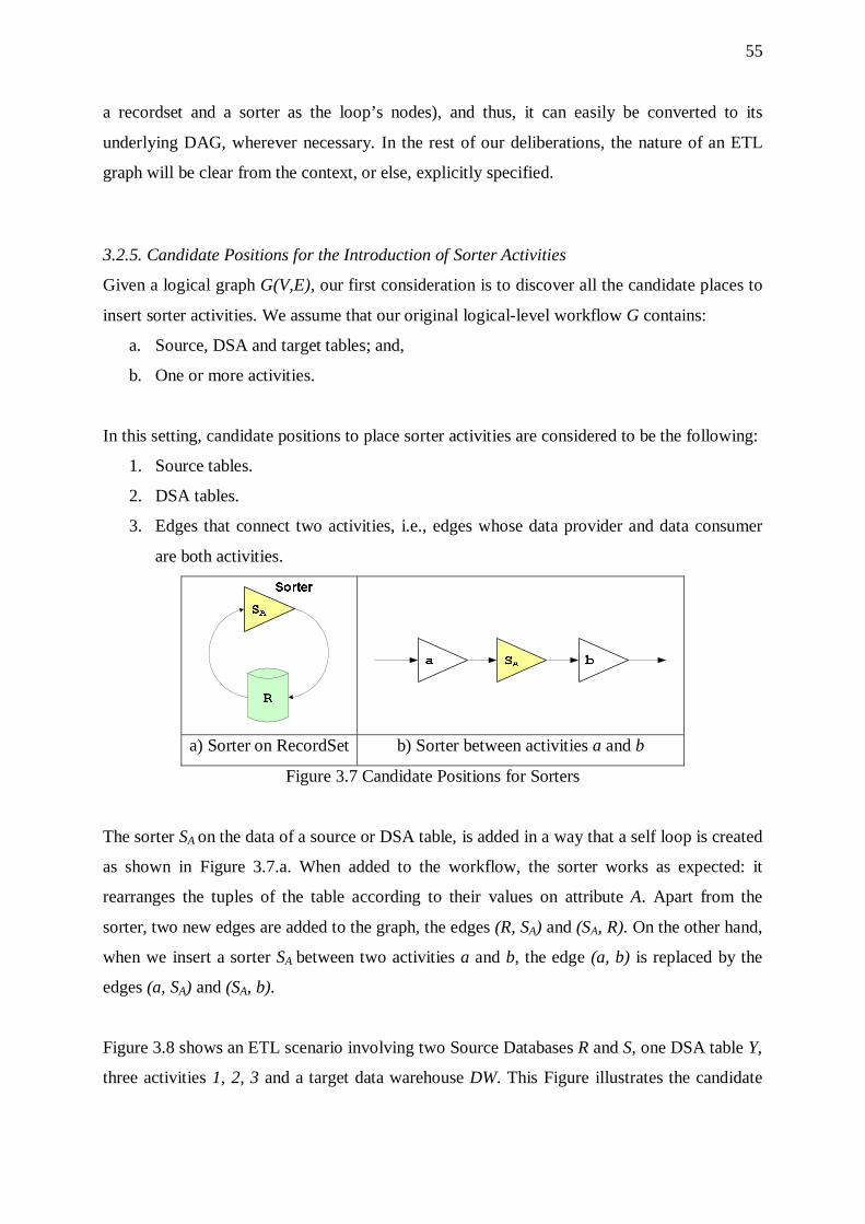
55

a recordset and a sorter as the loop’s nodes), and thus, it can easily be converted to its

underlying DAG, wherever necessary. In the rest of our deliberations, the nature of an ETL

graph will be clear from the context, or else, explicitly specified.

3.2.5. Candidate Positions for the Introduction of Sorter Activities

Given a logical graph G(V,E), our first consideration is to discover all the candidate places to

insert sorter activities. We assume that our original logical-level workflow G contains:

a. Source, DSA and target tables; and,

b. One or more activities.

In this setting, candidate positions to place sorter activities are considered to be the following:

1. Source tables.

2. DSA tables.

3. Edges that connect two activities, i.e., edges whose data provider and data consumer

are both activities.

a) Sorter on RecordSet b) Sorter between activities a and b

Figure 3.7 Candidate Positions for Sorters

The sorter SA on the data of a source or DSA table, is added in a way that a self loop is created

as shown in Figure 3.7.a. When added to the workflow, the sorter works as expected: it

rearranges the tuples of the table according to their values on attribute A. Apart from the

sorter, two new edges are added to the graph, the edges (R, SA) and (SA, R). On the other hand,

when we insert a sorter SA between two activities a and b, the edge (a, b) is replaced by the

edges (a, SA) and (SA, b).

Figure 3.8 shows an ETL scenario involving two Source Databases R and S, one DSA table Y,

three activities 1, 2, 3 and a target data warehouse DW. This Figure illustrates the candidate

56

positions to place sorter activities. Candidate positions for sorters are marked with letters

enclosed in parentheses (places (a) to (d), i.e., on the data of tables R, S and Y and on the edge

(1, 3)).

Figure 3.8 Candidate Places for Sorters

3.2.6. Selection of Candidate Attributes for Orderings

A second problem that needs to be solved, concerns the choice of the attributes of each

recordset’s schema/activity’s output schema accordingly, over which an ordering of data will

be performed.

We now define some terms that are useful to our approach. First, we discuss interesting

orders, whose critical role in cost-based query optimization has been recognized in

[SAC+79].

An interesting order for a set of tuples as defined in [SAC+79] is a specification for any

ordering of data that is important for query optimization. If we determine all interesting orders

for a set of tuples, we can form the set of interesting orders. In our setting, the set of

interesting orders consists of a list of attributes over which we can sort the input of an activity

or the contents of a recordset. Thus, the set of interesting orders consists of a set of candidate

attributes such that an ordering over any of these attributes is interesting (i.e., can be

beneficial for workflow optimization purposes).

Interesting Orders for ETL Activities

Our objective is to identify the set of interesting orders for each activity of the workflow. The

interesting orders for an activity are defined at physical-template level. Then, they are

57

customized per scenario. In other words, one of the properties of a physical-level template for

activities is the set of interesting orders for the activity. To construct the activity, the designer

specifies the activity and provides concrete values to the template parameters.

For example, when the designer of a workflow materializes a Not_Null template for the

activity with concrete semantics σNAME≠NULL, the physical template for Not_Null contains the

following elements:

1. Semantics (abstract): σ$≠NULL

2. Interesting Orders (abstract): $

Thus, the interesting order for Not_Null is instantiated as NAME.

We present more examples of interesting orders next:

1. For filters, each of the attributes involved in the check performed by the filter

composes an interesting order. E.g., the attribute A in the filter σA<1000 produces an

interesting order.

2. In case of a Join, (binary activity), each attribute that participates in the join condition

produces an interesting order. For the example join condition R.A = S.B both attributes

A and B that take part in the joining of tables R and S generate the interesting orders A

and B respectively.

3. We now examine the case of Aggregations. In such a case, each attribute in the

grouping-list produces an interesting order.

4. In case of a function that applies over a number of attributes, each of these attributes

produces an interesting order. Furthermore, each of the attributes produced by the

function, may compose an interesting order. Another thing to consider is that certain

activities do not produce any interesting order. For example, the function Convert$2€

does not have an interesting order. These activities are ignored in the whole process.

How to Determine Interesting Orders for Sorters

Having discussed ways to discover interesting orders for black-box ETL activities, we now

proceed to the case of sorters and describe a method to choose candidate attributes for sorter

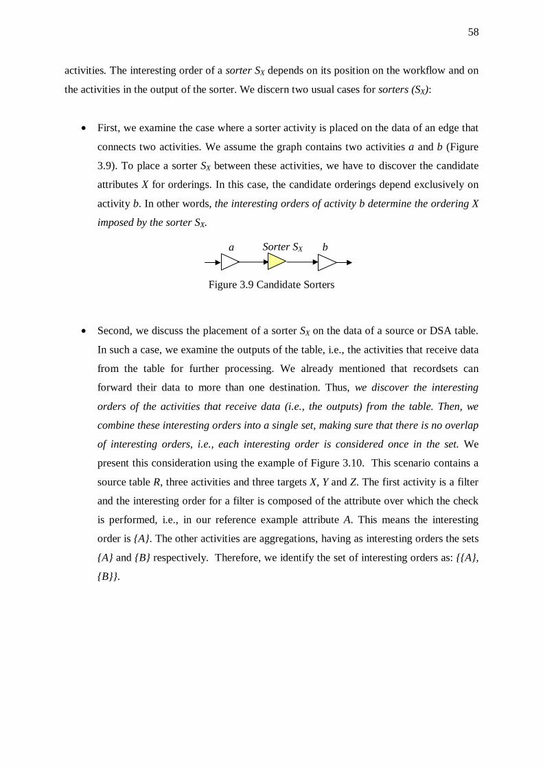
58

activities. The interesting order of a sorter SX depends on its position on the workflow and on

the activities in the output of the sorter. We discern two usual cases for sorters (SX):

• First, we examine the case where a sorter activity is placed on the data of an edge that

connects two activities. We assume the graph contains two activities a and b (Figure

3.9). To place a sorter SX between these activities, we have to discover the candidate

attributes X for orderings. In this case, the candidate orderings depend exclusively on

activity b. In other words, the interesting orders of activity b determine the ordering X

imposed by the sorter SX.

Figure 3.9 Candidate Sorters

• Second, we discuss the placement of a sorter SX on the data of a source or DSA table.

In such a case, we examine the outputs of the table, i.e., the activities that receive data

from the table for further processing. We already mentioned that recordsets can

forward their data to more than one destination. Thus, we discover the interesting

orders of the activities that receive data (i.e., the outputs) from the table. Then, we

combine these interesting orders into a single set, making sure that there is no overlap

of interesting orders, i.e., each interesting order is considered once in the set. We

present this consideration using the example of Figure 3.10. This scenario contains a

source table R, three activities and three targets X, Y and Z. The first activity is a filter

and the interesting order for a filter is composed of the attribute over which the check

is performed, i.e., in our reference example attribute A. This means the interesting

order is A. The other activities are aggregations, having as interesting orders the sets

A and B respectively. Therefore, we identify the set of interesting orders as: A,

B.

Sorter SX

a a

a b

a

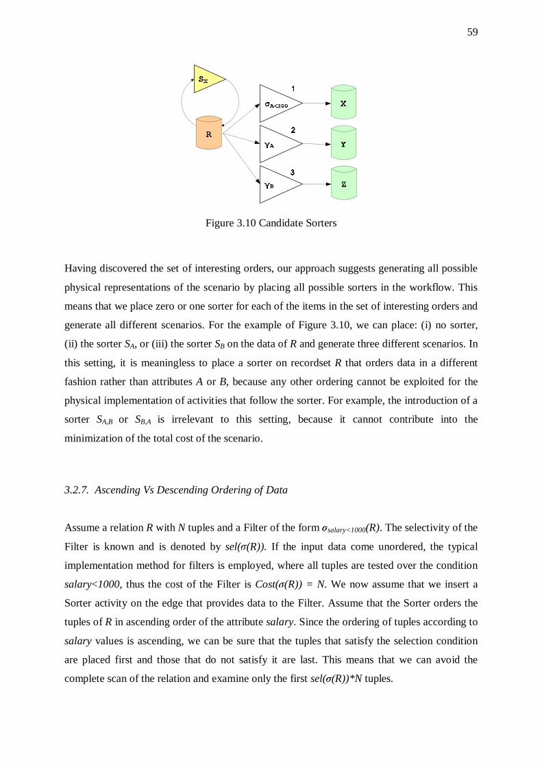
59

Figure 3.10 Candidate Sorters

Having discovered the set of interesting orders, our approach suggests generating all possible

physical representations of the scenario by placing all possible sorters in the workflow. This

means that we place zero or one sorter for each of the items in the set of interesting orders and

generate all different scenarios. For the example of Figure 3.10, we can place: (i) no sorter,

(ii) the sorter SA, or (iii) the sorter SB on the data of R and generate three different scenarios. In

this setting, it is meaningless to place a sorter on recordset R that orders data in a different

fashion rather than attributes A or B, because any other ordering cannot be exploited for the

physical implementation of activities that follow the sorter. For example, the introduction of a

sorter SA,B or SB,A is irrelevant to this setting, because it cannot contribute into the

minimization of the total cost of the scenario.

3.2.7. Ascending Vs Descending Ordering of Data

Assume a relation R with N tuples and a Filter of the form σsalary<1000(R). The selectivity of the

Filter is known and is denoted by sel(σ(R)). If the input data come unordered, the typical

implementation method for filters is employed, where all tuples are tested over the condition

salary<1000, thus the cost of the Filter is Cost(σ(R)) = N. We now assume that we insert a

Sorter activity on the edge that provides data to the Filter. Assume that the Sorter orders the

tuples of R in ascending order of the attribute salary. Since the ordering of tuples according to

salary values is ascending, we can be sure that the tuples that satisfy the selection condition

are placed first and those that do not satisfy it are last. This means that we can avoid the

complete scan of the relation and examine only the first sel(σ(R))*N tuples.

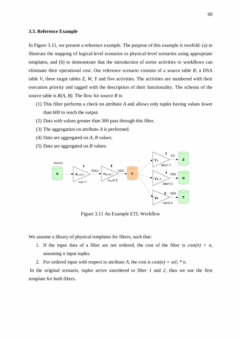
60

3.3. Reference Example

In Figure 3.11, we present a reference example. The purpose of this example is twofold: (a) to

illustrate the mapping of logical-level scenarios to physical-level scenarios using appropriate

templates, and (b) to demonstrate that the introduction of sorter activities to workflows can

eliminate their operational cost. Our reference scenario consists of a source table R, a DSA

table V, three target tables Z, W, Y and five activities. The activities are numbered with their

execution priority and tagged with the description of their functionality. The schema of the

source table is R(A, B). The flow for source R is:

(1) This filter performs a check on attribute A and allows only tuples having values lower

than 600 to reach the output.

(2) Data with values greater than 300 pass through this filter.

(3) The aggregation on attribute A is performed.

(4) Data are aggregated on A, B values.

(5) Data are aggregated on B values.

γA

3

VR

Z

σA>300

2

σA<600

1

γA,Β

4

W

100000

500

10000

1000

γB

5

Y

1000

5000

sel1=0.1sel2=0.5

sel3=0.1

sel4=0.2

sel5=0.2

Figure 3.11 An Example ETL Workflow

We assume a library of physical templates for filters, such that:

1. If the input data of a filter are not ordered, the cost of the filter is cost(σ) = n,

assuming n input tuples.

2. For ordered input with respect to attribute A, the cost is cost(σ) = sel1 * n.

In the original scenario, tuples arrive unordered to filter 1 and 2, thus we use the first

template for both filters.

61

Furthermore, we assume a library of physical templates for aggregations: NL, SO and HS. In

this example, the NL and the HS implementation are not feasible for activities 3 to 5, since

their output tuples do not meet the condition |output tuples|<√(|input tuples|). If we assume n

input tuples for an aggregation, then the cost of the sort-based implementation method is:

costSO(γ) = n*log2(n)+n

Based on the aforementioned cost formulae, we compute the cost of the original scenario:

Cost(G) =5

1( )

icost i

=∑ =100.000+10.000+3*[5.000*log2(5.000)+5.000] = 309.316

We continue to generate all possible physical implementations of the scenario and consider

candidate positions to place sorter activities. According to our approach, sorter activities can

be placed on the data of tables R and V, as well as on the edge (1, 2).

• For a sorter placed on the data of table R, the interesting order is A.

• For a sorter placed on edge (1, 2) the interesting order is A.

• For a sorter on the data of table V the interesting orders are: A, B, A, B, B, A.

Our approach suggests inserting combinations of the above sorters on the workflow and

computing relevant costs.

In the sequel, we do not explore all these alternative interesting orders. Specifically, assume

that we apply a transition ASR(SA,B, R) to generate an equivalent workflow G’. Thus, a sorter

SA,B is introduced on the data of table V of the workflow. Then, we observe changes imposed

by the sorter to the sort order of the tuples originating from V and reaching activities 3 to 5 for

further processing:

• We notice that activity 3 gets data ordered according to A,B. This means that data are

ordered according to the grouping attribute A. Thus, the cost of the aggregation is

reduced to: cost(3) = |input tuples| =5.000

• Similarly, the cost of 4 is reduced to: cost(4) = 5.000.

• The cost of activity 5 remains the same, since its input data are not ordered by B.

Thus, the cost of the workflow G’ can be computed as follows:

Cost(G’) =5

1( )

icost i

=∑ =100.000+10.000+2*5.000+[5.000*log2(5.000)+5.000] = 247.877

On the whole, we notice that Cost(G’)<Cost(G). This means that the transition ASR(SA,B, R)

has produced an equivalent workflow G’ with lower cost than the original scenario. In other

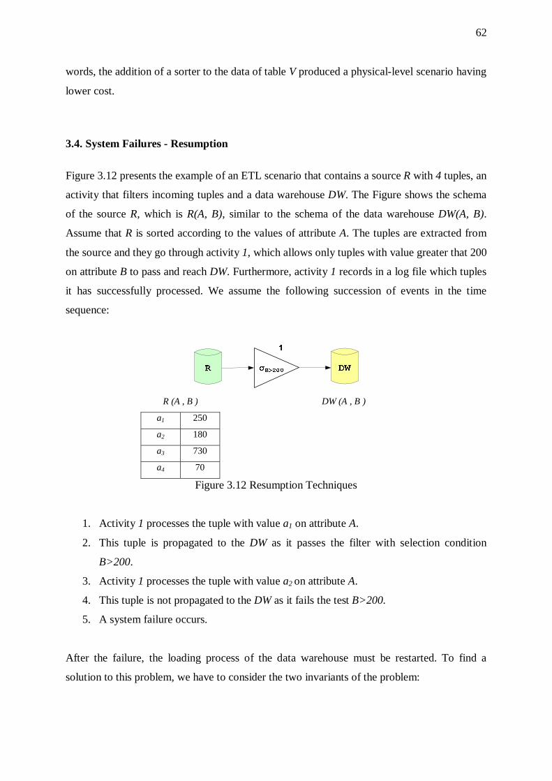
62

words, the addition of a sorter to the data of table V produced a physical-level scenario having

lower cost.

3.4. System Failures - Resumption

Figure 3.12 presents the example of an ETL scenario that contains a source R with 4 tuples, an

activity that filters incoming tuples and a data warehouse DW. The Figure shows the schema

of the source R, which is R(A, B), similar to the schema of the data warehouse DW(A, B).

Assume that R is sorted according to the values of attribute A. The tuples are extracted from

the source and they go through activity 1, which allows only tuples with value greater that 200

on attribute B to pass and reach DW. Furthermore, activity 1 records in a log file which tuples

it has successfully processed. We assume the following succession of events in the time

sequence:

DW (A , B )

Figure 3.12 Resumption Techniques

1. Activity 1 processes the tuple with value a1 on attribute A.

2. This tuple is propagated to the DW as it passes the filter with selection condition

B>200.

3. Activity 1 processes the tuple with value a2 on attribute A.

4. This tuple is not propagated to the DW as it fails the test B>200.

5. A system failure occurs.

After the failure, the loading process of the data warehouse must be restarted. To find a

solution to this problem, we have to consider the two invariants of the problem:

R (A , B )

a1 250

a2 180

a3 730

a4 70

63

- All the tuples of R must be processed and

- No duplicate records must reach the DW.

To answer the problem, there are two different techniques we can follow:

1. The first choice is to redo the entire load after the failure. This means to filter out the

already stored tuples at the warehouse and reprocess data in its entirety. If the whole

process manages to complete, then we hope that another failure does not occur.

2. The second option is to resume the incomplete load of DW, starting from the point it

was interrupted assuming that we can avoid redoing work with rescued output and we

know where to start.

The first option can be time consuming, since the loading of a data warehouse usually takes

hours or even days to complete. Moreover, if there is not enough time for the load to finish, it

may be skipped for a next period of time, leaving the database incomplete, possibly

inconsistent and out of date.

On the other hand, the second technique seems to be more convenient for this problem. We

now present its successive stages after a failure occurs. On system restart, activity 1 discovers

that DW contains only one tuple, the tuple with value a1 on attribute A. Since we know that

tuples are processed in alphabetical order by activity 1, we can exploit the fact that activity 1

“remembers” which tuples it has already processed. This means that after the failure, activity

1 does not have to reprocess tuples with values a1 and a2 on attribute A, so we continue by

retrieving tuples from R starting from the ones with value a3 on attribute A.

We assume that system failures happen during the operation of the workflow. To overcome

the obstacles that failures cause to the warehouse load, we suppose that each DSA table plays

the role of a savepoint of the workflow state. Each DSA table stores an amount of processed

data and when a failure occurs, the DSA table makes this data available to the activities

following it in the workflow. Each activity refers to the latest DSA savepoint to extract tuples

for processing. In other words, each DSA recordset serves as a bridge that in case of a failure

provides all activities that follow it in the workflow with the most recently saved data, ready

for further processing.

In case the workflow does not contain any DSA tables, the workflow operation must be

restarted from scratch, i.e., each activity has to reprocess all input tuples. On the other hand, if

64

the workflow contains savepoints, an activity that fails to complete its operation can receive

input data from its closest DSA savepoint. Assume that activity i fails during processing.

Then, activity i refers to its closest DSA table and receives tuples from it. In this case, not all

activities have to restart their work. Only activity i and the activities that follow it in the

workflow must resume their operation. This means that the cost to resume the workflow

operation can be lower due to the existence of savepoints. Thus, the use of savepoints is

beneficial in most cases.

65

CHAPTER 4. TECHNICAL ISSUES AND PROPOSED

ALGORITHMS

4.1 Architecture of the Implemented ETL Engine

4.2 Technical Issues – Proposed Algorithms

4.3 Alternative Cost Models

4.4 Implementation Issues

In this section, we present the architecture of our ETL engine. Then, we discuss signatures,

which provide a compact way to represent a scenario with a string. In addition, we refer to the

algorithms used in our approach and present the algorithm Exhaustive Ordering. We present

two different cost models, one for the regular operation of an ETL workflow and another with

recovery from failures. Furthermore, we introduce the language DEWL for the description of

ETL scenarios and describe its syntax. Finally, we describe the construction of a parser for

language DEWL.

4.1. Architecture of the Implemented ETL Engine

We described in previous sections that ETL tools are software tools responsible for the

extraction of information from different sources, their transformation and cleansing and

finally their loading into the target data warehouse. Most ETL tools are either engine-based,

or code-generation based. According to the engine-based approach all data have to go

through an engine for transformation and processing. This means that all processing takes

place in the engine, which typically runs on a single machine. On the other hand, in code-

generating tools all processing takes place only at the target or source systems.

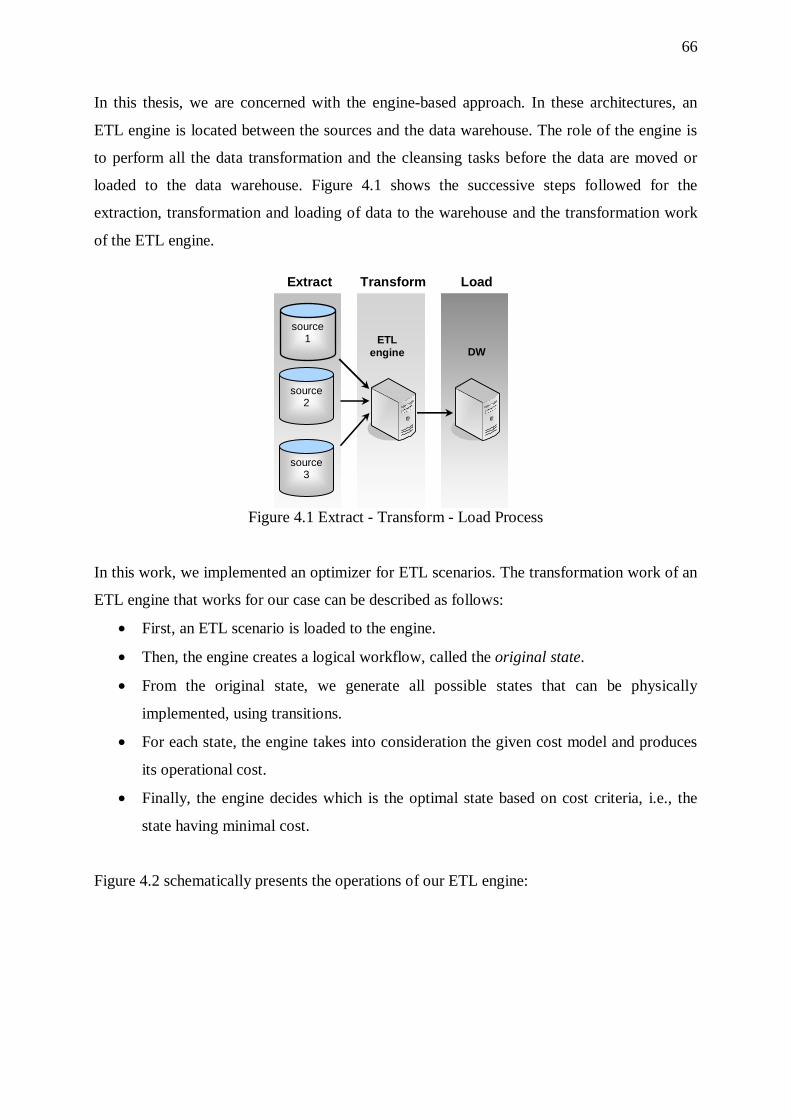
66

In this thesis, we are concerned with the engine-based approach. In these architectures, an

ETL engine is located between the sources and the data warehouse. The role of the engine is

to perform all the data transformation and the cleansing tasks before the data are moved or

loaded to the data warehouse. Figure 4.1 shows the successive steps followed for the

extraction, transformation and loading of data to the warehouse and the transformation work

of the ETL engine.

Figure 4.1 Extract - Transform - Load Process

In this work, we implemented an optimizer for ETL scenarios. The transformation work of an

ETL engine that works for our case can be described as follows:

• First, an ETL scenario is loaded to the engine.

• Then, the engine creates a logical workflow, called the original state.

• From the original state, we generate all possible states that can be physically

implemented, using transitions.

• For each state, the engine takes into consideration the given cost model and produces

its operational cost.

• Finally, the engine decides which is the optimal state based on cost criteria, i.e., the

state having minimal cost.

Figure 4.2 schematically presents the operations of our ETL engine:

Load Transform

ETL engine

source 1

Extract

source 2

source 3

DW

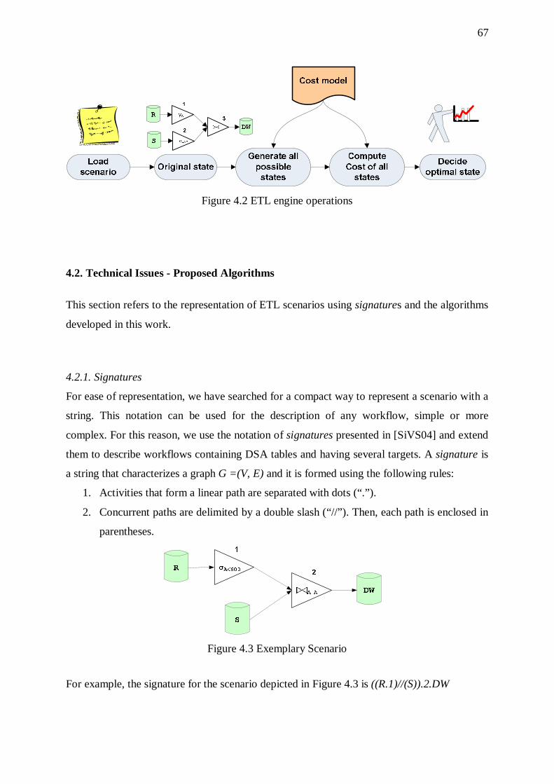
67

Figure 4.2 ETL engine operations

4.2. Technical Issues - Proposed Algorithms

This section refers to the representation of ETL scenarios using signatures and the algorithms

developed in this work.

4.2.1. Signatures

For ease of representation, we have searched for a compact way to represent a scenario with a

string. This notation can be used for the description of any workflow, simple or more

complex. For this reason, we use the notation of signatures presented in [SiVS04] and extend

them to describe workflows containing DSA tables and having several targets. A signature is

a string that characterizes a graph G =(V, E) and it is formed using the following rules:

1. Activities that form a linear path are separated with dots (“.”).

2. Concurrent paths are delimited by a double slash (“//”). Then, each path is enclosed in

parentheses.

DW

S

R σA<600

1

A=A

2

Figure 4.3 Exemplary Scenario

For example, the signature for the scenario depicted in Figure 4.3 is ((R.1)//(S)).2.DW

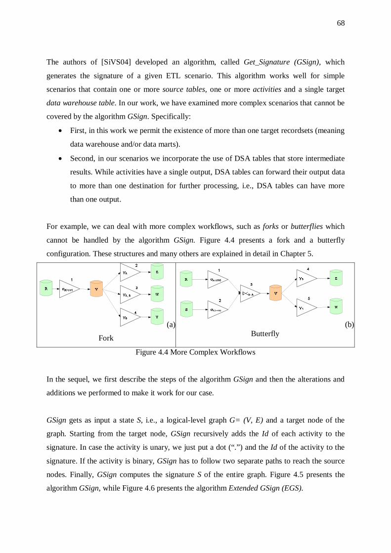
68

The authors of [SiVS04] developed an algorithm, called Get_Signature (GSign), which

generates the signature of a given ETL scenario. This algorithm works well for simple

scenarios that contain one or more source tables, one or more activities and a single target

data warehouse table. In our work, we have examined more complex scenarios that cannot be

covered by the algorithm GSign. Specifically:

• First, in this work we permit the existence of more than one target recordsets (meaning

data warehouse and/or data marts).

• Second, in our scenarios we incorporate the use of DSA tables that store intermediate

results. While activities have a single output, DSA tables can forward their output data

to more than one destination for further processing, i.e., DSA tables can have more

than one output.

For example, we can deal with more complex workflows, such as forks or butterflies which

cannot be handled by the algorithm GSign. Figure 4.4 presents a fork and a butterfly

configuration. These structures and many others are explained in detail in Chapter 5.

γA

2

V

Z

σA>300

1

γA,Β

3

W

γB

4

Y

R

(a)

Fork

(b) Butterfly

Figure 4.4 More Complex Workflows

In the sequel, we first describe the steps of the algorithm GSign and then the alterations and

additions we performed to make it work for our case.

GSign gets as input a state S, i.e., a logical-level graph G= (V, E) and a target node of the

graph. Starting from the target node, GSign recursively adds the Id of each activity to the

signature. In case the activity is unary, we just put a dot (“.”) and the Id of the activity to the

signature. If the activity is binary, GSign has to follow two separate paths to reach the source

nodes. Finally, GSign computes the signature S of the entire graph. Figure 4.5 presents the

algorithm GSign, while Figure 4.6 presents the algorithm Extended GSign (EGS).

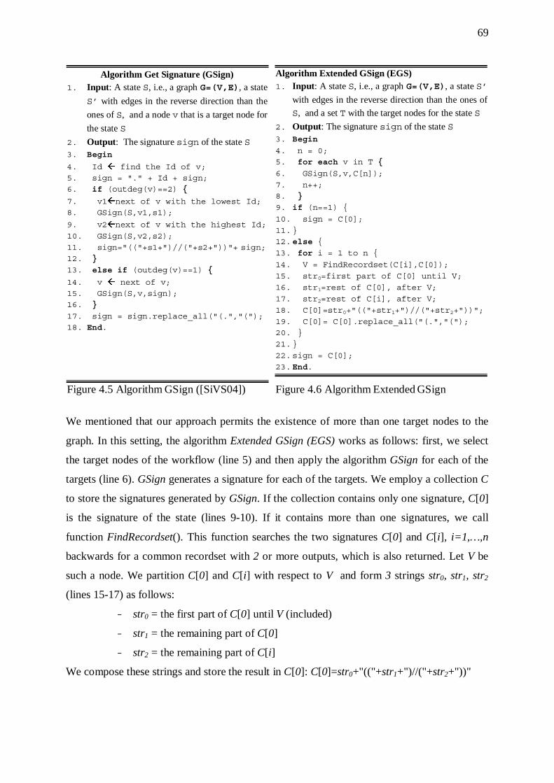
69

Algorithm Get Signature (GSign) 1. Input: A state S, i.e., a graph G=(V,E), a state

S’ with edges in the reverse direction than the

ones of S, and a node v that is a target node for

the state S

2. Output: The signature sign of the state S 3. Begin

4. Id find the Id of v; 5. sign = "." + Id + sign; 6. if (outdeg(v)==2)

7. v1next of v with the lowest Id; 8. GSign(S,v1,s1);

9. v2next of v with the highest Id;

10. GSign(S,v2,s2); 11. sign="(("+s1+")//("+s2+"))"+ sign; 12. 13. else if (outdeg(v)==1)

14. v next of v; 15. GSign(S,v,sign); 16. 17. sign = sign.replace_all("(.","("); 18. End.

Algorithm Extended GSign (EGS) 1. Input: A state S, i.e., a graph G=(V,E), a state S’

with edges in the reverse direction than the ones of

S, and a set T with the target nodes for the state S

2. Output: The signature sign of the state S 3. Begin 4. n = 0; 5. for each v in T 6. GSign(S,v,C[n]); 7. n++; 8. 9. if (n==1) 10. sign = C[0]; 11. 12. else 13. for i = 1 to n 14. V = FindRecordset(C[i],C[0]); 15. str0=first part of C[0] until V; 16. str1=rest of C[0], after V; 17. str2=rest of C[i], after V; 18. C[0]=str0+"(("+str1+")//("+str2+"))";19. C[0]= C[0].replace_all("(.","("); 20. 21. 22. sign = C[0]; 23. End.

Figure 4.5 Algorithm GSign ([SiVS04]) Figure 4.6 Algorithm Extended GSign

We mentioned that our approach permits the existence of more than one target nodes to the

graph. In this setting, the algorithm Extended GSign (EGS) works as follows: first, we select

the target nodes of the workflow (line 5) and then apply the algorithm GSign for each of the

targets (line 6). GSign generates a signature for each of the targets. We employ a collection C

to store the signatures generated by GSign. If the collection contains only one signature, C[0]

is the signature of the state (lines 9-10). If it contains more than one signatures, we call

function FindRecordset(). This function searches the two signatures C[0] and C[i], i=1,…,n

backwards for a common recordset with 2 or more outputs, which is also returned. Let V be

such a node. We partition C[0] and C[i] with respect to V and form 3 strings str0, str1, str2

(lines 15-17) as follows:

- str0 = the first part of C[0] until V (included)

- str1 = the remaining part of C[0]

- str2 = the remaining part of C[i]

We compose these strings and store the result in C[0]: C[0]=str0+"(("+str1+")//("+str2+"))"

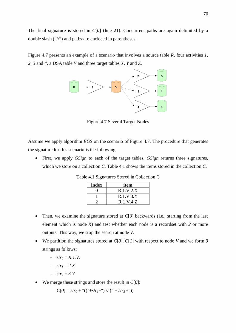
70

The final signature is stored in C[0] (line 21). Concurrent paths are again delimited by a

double slash (“//”) and paths are enclosed in parentheses.

Figure 4.7 presents an example of a scenario that involves a source table R, four activities 1,

2, 3 and 4, a DSA table V and three target tables X, Y and Z.

Figure 4.7 Several Target Nodes

Assume we apply algorithm EGS on the scenario of Figure 4.7. The procedure that generates

the signature for this scenario is the following:

• First, we apply GSign to each of the target tables. GSign returns three signatures,

which we store on a collection C. Table 4.1 shows the items stored in the collection C.

Table 4.1 Signatures Stored in Collection C

index item 0 R.1.V.2.X 1 R.1.V.3.Y 2 R.1.V.4.Z

• Then, we examine the signature stored at C[0] backwards (i.e., starting from the last

element which is node X) and test whether each node is a recordset with 2 or more

outputs. This way, we stop the search at node V.

• We partition the signatures stored at C[0], C[1] with respect to node V and we form 3

strings as follows:

- str0 = R.1.V.

- str1 = 2.X

- str2 = 3.Y

• We merge these strings and store the result in C[0]:

C[0] = str0 + "(("+str1+") // (" + str2 +"))"

71

• Similarly, we test each remaining signature stored at C with C[0] and merge strings.

• Thus, the final signature is: R.1.V. ((((2.X)//(3.Y)))//(4.Z))

Extensions to Extended GSign To adjust the algorithm Extended GSign to cover all possible scenarios in our setting, we

made the following extensions:

1. First, we incorporated physical-level activities to signatures and adjusted the algorithm

EGS to generate such signatures.

2. Second, we extended the algorithm EGS to work for workflows that contain sorter

activities.

For the first case, we present an example using the scenario of Figure 4.7. Assume that the

aggregation is performed using a NL implementation method. Then, the signature of the

scenario generated by EGS is R.1.V.((2@NL.W)//(3.Z)). This example shows that EGS uses

the notation introduced in section 3.1.3 for physical-level activities.

For the latter case, we have to mention how the algorithm is extended when sorters are

present.

• Whenever a sorter that orders data according to attributes A,B is placed on an edge (a,

b), where a, b are activities, we name the sorter a_b and the signature contains the

notation a_b(A,B) to convey the sorter.

• On the other hand, if we introduce a sorter on table V that orders tuples according to

A,B the signature contains the notation V!(A,B) using the separator “!” to differentiate

the name of the sorter from the ordering attributes.

4.2.2. Algorithm Generate Possible Orders (GPO)

The designer of a new scenario has to provide to the system information concerning the

logical description of the scenario. This means that he has to describe analytically all the

recordsets and activities contained in the scenario and their interconnections (by referring to

inputs/outputs of activities). This way the ETL engine can initiate its transformation work.

Furthermore, some additional information is needed for each type of activity. The designer

needs to specify a comma delimited list of parameters, which correspond to the set of

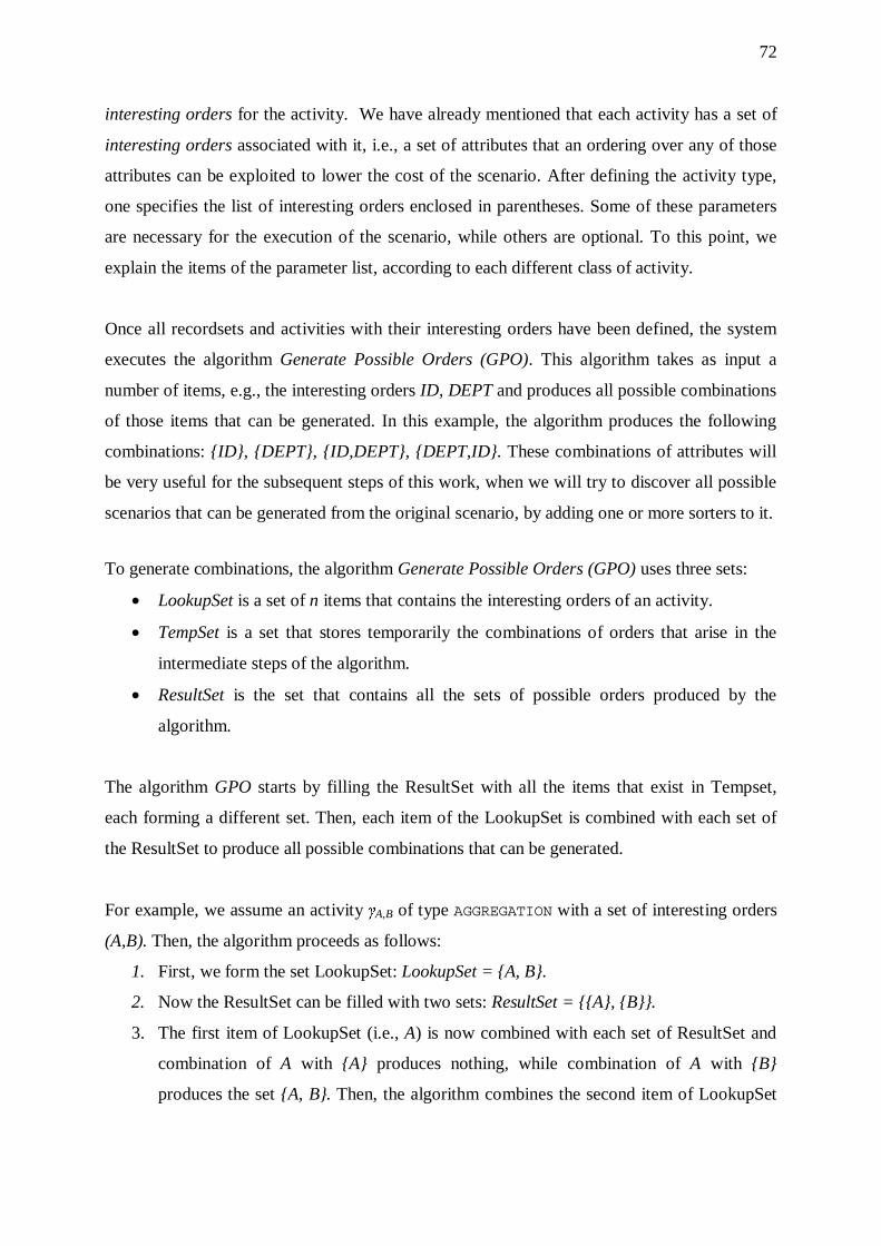
72

interesting orders for the activity. We have already mentioned that each activity has a set of

interesting orders associated with it, i.e., a set of attributes that an ordering over any of those

attributes can be exploited to lower the cost of the scenario. After defining the activity type,

one specifies the list of interesting orders enclosed in parentheses. Some of these parameters

are necessary for the execution of the scenario, while others are optional. To this point, we

explain the items of the parameter list, according to each different class of activity.

Once all recordsets and activities with their interesting orders have been defined, the system

executes the algorithm Generate Possible Orders (GPO). This algorithm takes as input a

number of items, e.g., the interesting orders ID, DEPT and produces all possible combinations

of those items that can be generated. In this example, the algorithm produces the following

combinations: ID, DEPT, ID,DEPT, DEPT,ID. These combinations of attributes will

be very useful for the subsequent steps of this work, when we will try to discover all possible

scenarios that can be generated from the original scenario, by adding one or more sorters to it.

To generate combinations, the algorithm Generate Possible Orders (GPO) uses three sets:

• LookupSet is a set of n items that contains the interesting orders of an activity.

• TempSet is a set that stores temporarily the combinations of orders that arise in the

intermediate steps of the algorithm.

• ResultSet is the set that contains all the sets of possible orders produced by the

algorithm.

The algorithm GPO starts by filling the ResultSet with all the items that exist in Tempset,

each forming a different set. Then, each item of the LookupSet is combined with each set of

the ResultSet to produce all possible combinations that can be generated.

For example, we assume an activity γA,B of type AGGREGATION with a set of interesting orders

(A,B). Then, the algorithm proceeds as follows:

1. First, we form the set LookupSet: LookupSet = A, B.

2. Now the ResultSet can be filled with two sets: ResultSet = A, B.

3. The first item of LookupSet (i.e., A) is now combined with each set of ResultSet and

combination of A with A produces nothing, while combination of A with B

produces the set A, B. Then, the algorithm combines the second item of LookupSet

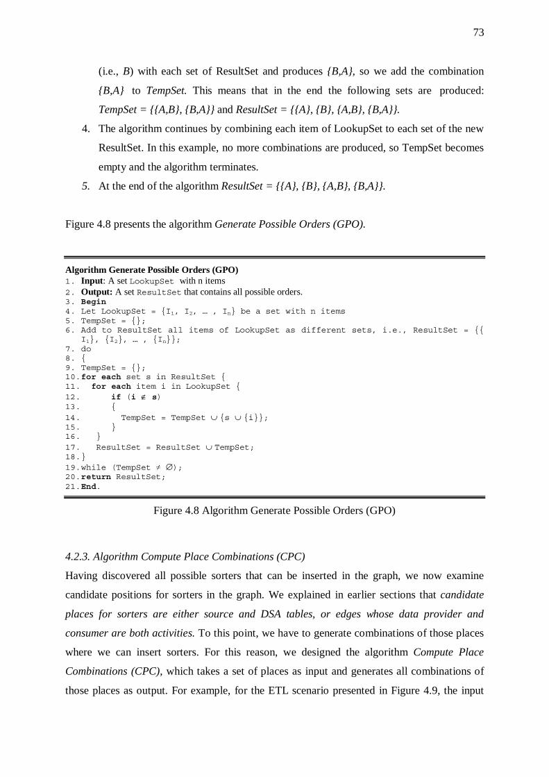
73

(i.e., B) with each set of ResultSet and produces B,A, so we add the combination

B,A to TempSet. This means that in the end the following sets are produced:

TempSet = A,B, B,A and ResultSet = A, B, A,B, B,A.

4. The algorithm continues by combining each item of LookupSet to each set of the new

ResultSet. In this example, no more combinations are produced, so TempSet becomes

empty and the algorithm terminates.

5. At the end of the algorithm ResultSet = A, B, A,B, B,A.

Figure 4.8 presents the algorithm Generate Possible Orders (GPO).

Algorithm Generate Possible Orders (GPO) 1. Input: A set LookupSet with n items 2. Output: A set ResultSet that contains all possible orders. 3. Begin 4. Let LookupSet = I1, I2, … , In be a set with n items 5. TempSet = ; 6. Add to ResultSet all items of LookupSet as different sets, i.e., ResultSet =

I1, I2, … , In; 7. do 8. 9. TempSet = ; 10. for each set s in ResultSet 11. for each item i in LookupSet 12. if (i ∉ s) 13. 14. TempSet = TempSet ∪ s ∪ i; 15. 16. 17. ResultSet = ResultSet ∪ TempSet; 18. 19. while (TempSet ≠ ∅); 20. return ResultSet; 21. End.

Figure 4.8 Algorithm Generate Possible Orders (GPO)

4.2.3. Algorithm Compute Place Combinations (CPC)

Having discovered all possible sorters that can be inserted in the graph, we now examine

candidate positions for sorters in the graph. We explained in earlier sections that candidate

places for sorters are either source and DSA tables, or edges whose data provider and

consumer are both activities. To this point, we have to generate combinations of those places

where we can insert sorters. For this reason, we designed the algorithm Compute Place

Combinations (CPC), which takes a set of places as input and generates all combinations of

those places as output. For example, for the ETL scenario presented in Figure 4.9, the input

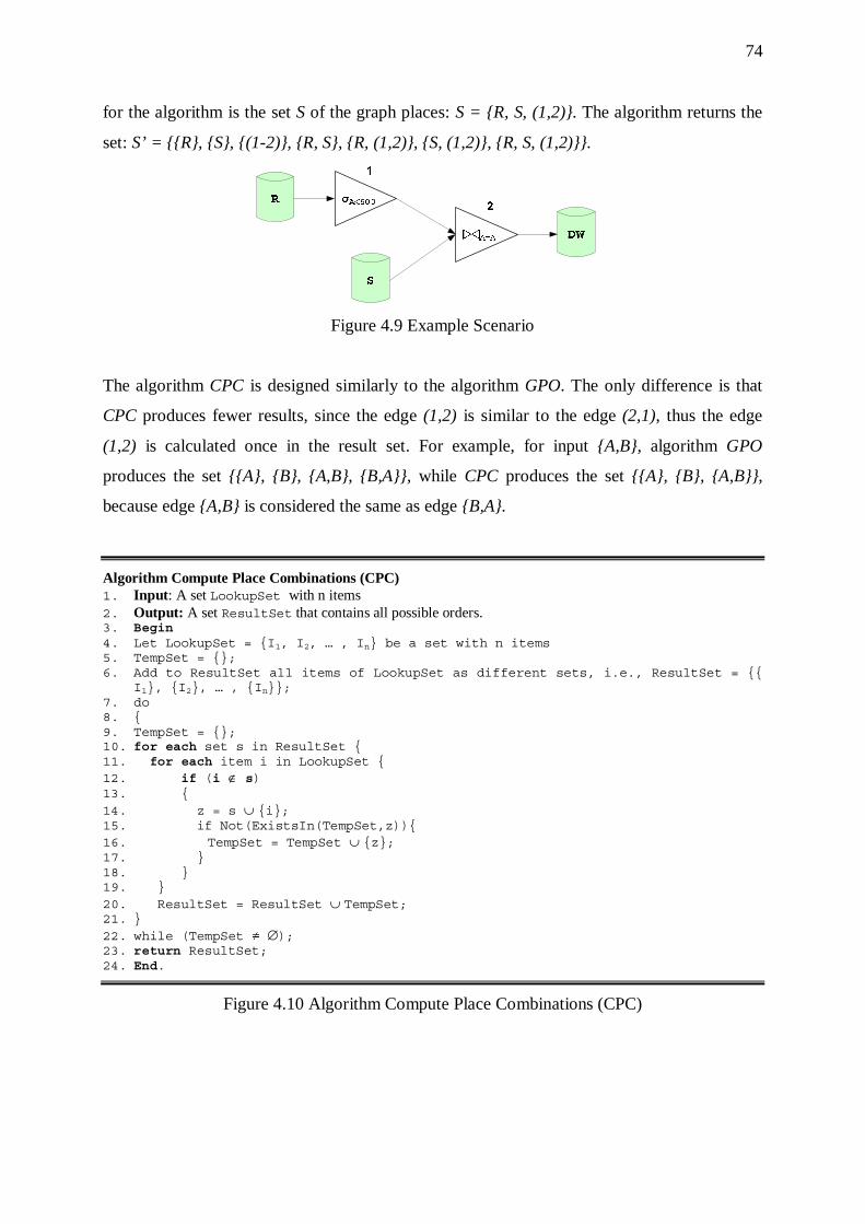
74

for the algorithm is the set S of the graph places: S = R, S, (1,2). The algorithm returns the

set: S’ = R, S, (1-2), R, S, R, (1,2), S, (1,2), R, S, (1,2).

DW

S

R σA<600

1

A=A

2

Figure 4.9 Example Scenario

The algorithm CPC is designed similarly to the algorithm GPO. The only difference is that

CPC produces fewer results, since the edge (1,2) is similar to the edge (2,1), thus the edge

(1,2) is calculated once in the result set. For example, for input A,B, algorithm GPO

produces the set A, B, A,B, B,A, while CPC produces the set A, B, A,B,

because edge A,B is considered the same as edge B,A.

Algorithm Compute Place Combinations (CPC) 1. Input: A set LookupSet with n items 2. Output: A set ResultSet that contains all possible orders. 3. Begin 4. Let LookupSet = I1, I2, … , In be a set with n items 5. TempSet = ; 6. Add to ResultSet all items of LookupSet as different sets, i.e., ResultSet =

I1, I2, … , In; 7. do 8. 9. TempSet = ; 10. for each set s in ResultSet 11. for each item i in LookupSet 12. if (i ∉ s) 13. 14. z = s ∪ i; 15. if Not(ExistsIn(TempSet,z)) 16. TempSet = TempSet ∪ z; 17. 18. 19. 20. ResultSet = ResultSet ∪ TempSet; 21. 22. while (TempSet ≠ ∅); 23. return ResultSet; 24. End.

Figure 4.10 Algorithm Compute Place Combinations (CPC)

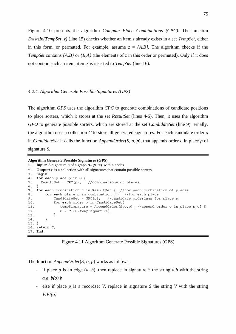
75

Figure 4.10 presents the algorithm Compute Place Combinations (CPC). The function

ExistsIn(TempSet, z) (line 15) checks whether an item z already exists in a set TempSet, either

in this form, or permuted. For example, assume z = A,B. The algorithm checks if the

TempSet contains A,B or B,A (the elements of z in this order or permuted). Only if it does

not contain such an item, item z is inserted to TempSet (line 16).

4.2.4. Algorithm Generate Possible Signatures (GPS)

The algorithm GPS uses the algorithm CPC to generate combinations of candidate positions

to place sorters, which it stores at the set ResultSet (lines 4-6). Then, it uses the algorithm

GPO to generate possible sorters, which are stored at the set CandidateSet (line 9). Finally,

the algorithm uses a collection C to store all generated signatures. For each candidate order o

in CandidateSet it calls the function AppendOrder(S, o, p), that appends order o in place p of

signature S.

Algorithm Generate Possible Signatures (GPS) 1. Input: A signature S of a graph G=(V,E) with n nodes 2. Output: C is a collection with all signatures that contain possible sorters. 3. Begin 4. for each place p in G 5. ResultSet = CPC(p); //combinations of places 6. 7. for each combination c in ResultSet //for each combination of places 8. for each place p in combination c //for each place 9. CandidateSet = GPO(p); //candidate orderings for place p 10. for each order o in CandidateSet 11. tempSignature = AppendOrder(S,o,p); //append order o in place p of S 12. C = C ∪ tempSignature; 13. 14. 15. 16. return C; 17. End.

Figure 4.11 Algorithm Generate Possible Signatures (GPS)

The function AppendOrder(S, o, p) works as follows:

- if place p is an edge (a, b), then replace in signature S the string a.b with the string

a.a_b(o).b

- else if place p is a recordset V, replace in signature S the string V with the string

V.V!(o)

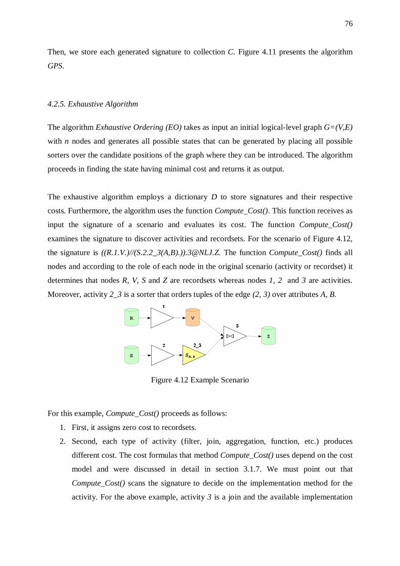
76

Then, we store each generated signature to collection C. Figure 4.11 presents the algorithm

GPS.

4.2.5. Exhaustive Algorithm

The algorithm Exhaustive Ordering (EO) takes as input an initial logical-level graph G=(V,E)

with n nodes and generates all possible states that can be generated by placing all possible

sorters over the candidate positions of the graph where they can be introduced. The algorithm

proceeds in finding the state having minimal cost and returns it as output.

The exhaustive algorithm employs a dictionary D to store signatures and their respective

costs. Furthermore, the algorithm uses the function Compute_Cost(). This function receives as

input the signature of a scenario and evaluates its cost. The function Compute_Cost()

examines the signature to discover activities and recordsets. For the scenario of Figure 4.12,

the signature is ((R.1.V.)//(S.2.2_3(A,B).)).3@NLJ.Z. The function Compute_Cost() finds all

nodes and according to the role of each node in the original scenario (activity or recordset) it

determines that nodes R, V, S and Z are recordsets whereas nodes 1, 2 and 3 are activities.

Moreover, activity 2_3 is a sorter that orders tuples of the edge (2, 3) over attributes A, B.

Figure 4.12 Example Scenario

For this example, Compute_Cost() proceeds as follows:

1. First, it assigns zero cost to recordsets.

2. Second, each type of activity (filter, join, aggregation, function, etc.) produces

different cost. The cost formulas that method Compute_Cost() uses depend on the cost

model and were discussed in detail in section 3.1.7. We must point out that

Compute_Cost() scans the signature to decide on the implementation method for the

activity. For the above example, activity 3 is a join and the available implementation

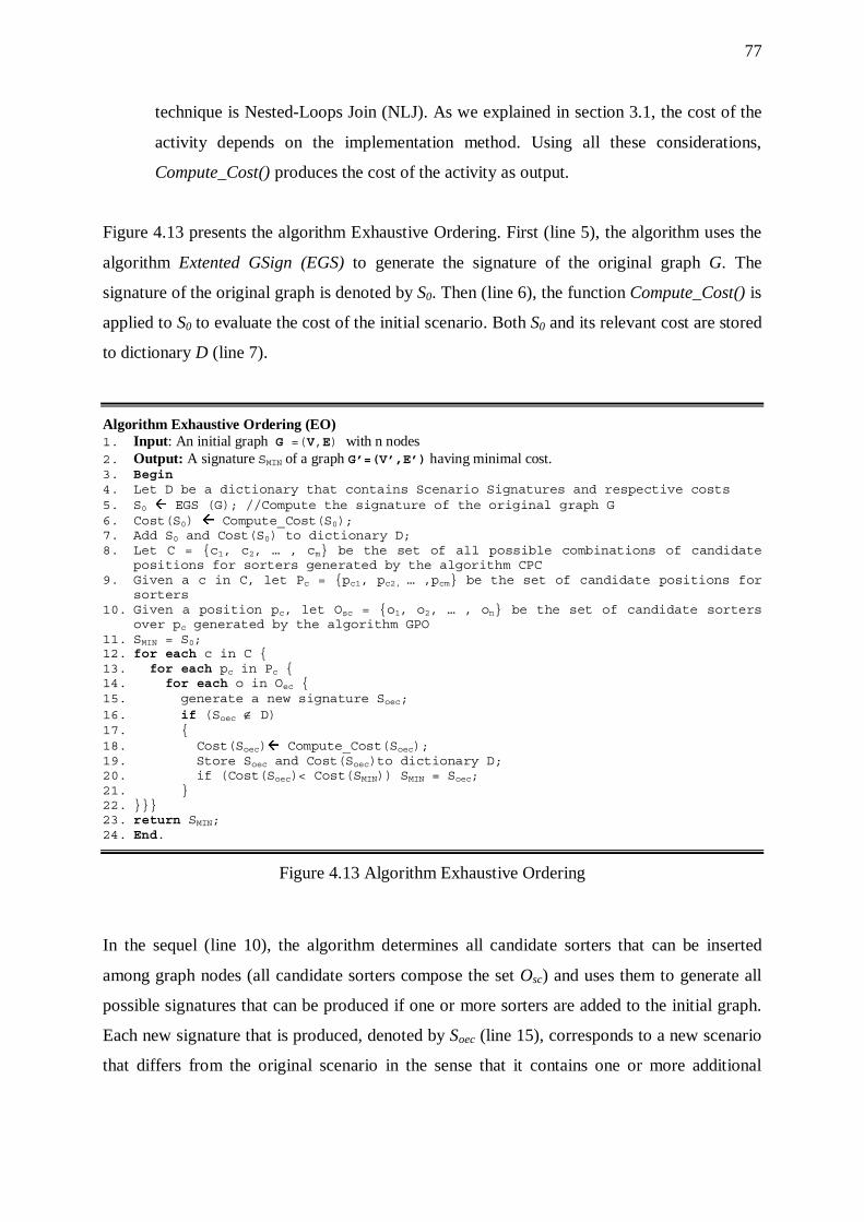
77

technique is Nested-Loops Join (NLJ). As we explained in section 3.1, the cost of the

activity depends on the implementation method. Using all these considerations,

Compute_Cost() produces the cost of the activity as output.

Figure 4.13 presents the algorithm Exhaustive Ordering. First (line 5), the algorithm uses the

algorithm Extented GSign (EGS) to generate the signature of the original graph G. The

signature of the original graph is denoted by S0. Then (line 6), the function Compute_Cost() is

applied to S0 to evaluate the cost of the initial scenario. Both S0 and its relevant cost are stored

to dictionary D (line 7).

Algorithm Exhaustive Ordering (EO) 1. Input: An initial graph G =(V,E) with n nodes 2. Output: A signature SMIN of a graph G’=(V’,E’) having minimal cost. 3. Begin 4. Let D be a dictionary that contains Scenario Signatures and respective costs 5. S0 EGS (G); //Compute the signature of the original graph G 6. Cost(S0) Compute_Cost(S0); 7. Add S0 and Cost(S0) to dictionary D; 8. Let C = c1, c2, … , cm be the set of all possible combinations of candidate

positions for sorters generated by the algorithm CPC 9. Given a c in C, let Pc = pc1, pc2, … ,pcm be the set of candidate positions for

sorters 10. Given a position pc, let Osc = o1, o2, … , on be the set of candidate sorters

over pc generated by the algorithm GPO 11. SMIN = S0; 12. for each c in C 13. for each pc in Pc 14. for each o in Oec 15. generate a new signature Soec; 16. if (Soec ∉ D) 17. 18. Cost(Soec) Compute_Cost(Soec); 19. Store Soec and Cost(Soec)to dictionary D; 20. if (Cost(Soec)< Cost(SMIN)) SMIN = Soec; 21. 22. 23. return SMIN; 24. End.

Figure 4.13 Algorithm Exhaustive Ordering

In the sequel (line 10), the algorithm determines all candidate sorters that can be inserted

among graph nodes (all candidate sorters compose the set Osc) and uses them to generate all

possible signatures that can be produced if one or more sorters are added to the initial graph.

Each new signature that is produced, denoted by Soec (line 15), corresponds to a new scenario

that differs from the original scenario in the sense that it contains one or more additional

78

sorter activities. It also differs from the original scenario, because it contains implementation

methods for the activities. This is shown by the abbreviations NLJ, SMJ, etc. that follow the

name of the activity in the signature, e.g., 3@NLJ. We exploit all this information gathered by

scanning each generated signature in line 18 of the Exhaustive Algorithm, when we apply the

function Compute_Cost() to the new signature to compute the cost of each generated scenario.

Then (line 16), the algorithm checks if the new signature Soec already exists in dictionary D. If

not, the algorithm computes the cost of the scenario that corresponds to signature Soec and

adds the Soec and its cost to the dictionary (lines 18-19). Finally (line 20), the algorithm

searches among signatures in the dictionary to check whether the newly inserted one has a

minimal cost. This way, the algorithm chooses the signature having the minimal cost (SMIN) as

the solution to our problem.

4.3. Alternative Cost Models

We now illustrate the different cost models we have incorporated in this work. The first

model is based only on operational/computational cost, i.e., the cost for each activity to

process incoming tuples. We refer to this model as the model for regular operation. On the

other hand, the second model, computes not only the operational cost for each activity, but

also the cost to resume it in case of failure. This model is referred to as regular operation with

recovery from failures. We discuss both models in the following sections.

4.3.1. Regular Operation

As a first approach, we have used a simple cost model. This model takes into consideration

only the operational/computational cost for each activity, i.e., the number of tuples the activity

has to process and it is based on simple formulae. These considerations are explained in more

detail below:

1. We assume that each recordset has zero computational cost, since recordsets are used

for data storage purposes.

2. For activities with known semantics, the computational_cost of the activity is the

number of tuples it has to process. Assume m input tuples. The computational_cost of

activity i depends on the physical implementation of the activity. Thus, it is defined at

79

physical template level as a function of m. In section 3.1.7 we have explained how the

computational_cost is computed for some classical categories of activities: filters,

joins, aggregations and function applications.

3. For black-box activities with unknown semantics, we can use the following formula:

computational_cost(i) =m* cost_per_tuple(i)

where m is the number of input tuples and cost_per_tuple(i) is the cost for activity i to

process a single record.

4. Assume a workflow G with n activities. Then, the total computational cost for the

entire workflow G(V,E) is obtained by summarizing the computational costs of all its

activities. The total computational cost is given by the following formula:

Computational_cost(G) = 1

_ ( )n

icomputational cost i

=∑

4.3.2. Regular Operation with Recovery from Failures

Apart from the regular operation of an ETL workflow, real-world scenarios involve the

resumption of the workflow in the case of failures [LiSt93]. The resumption process can be

accelerated if the results of the workflow are stored at intermediate storage points (a.k.a.

savepoints in the database literature). Clearly, if an activity fails to complete its operation it

can receive input data from its closest DSA savepoint. Assume that activity i fails during

processing. Then, activity i refers to its closest DSA table and receives tuples from it. In this

case, not all activities have to restart their work. Only activity i and the activities that follow it

in the workflow must resume their operation. This means that the cost to resume the workflow

operation can be lower due to the existence of savepoints. Thus, the use of savepoints is

beneficial in most cases.

We can design a resumption-effective ETL process as follows:

1. Assume that the cost to process incoming tuples for each activity i is

computational_cost(i).

2. Assume that each activity has already processed the 50% of input tuples before the

failure occurs. We denote by cost_until_crash(i) for activity i the cost for processing

of the 50% of tuples before the failure.

cost_until_crash(i) = 50% * computational_cost(i)

80

3. A failure occurs in activity i and it fails to complete its operation. Assume k activities

in the path from activity i to the latest savepoint. Their work must be repeated.

Furthermore, assume that m activities follow activity i in the path towards the data

warehouse. Then, the work of i and the work of all m subsequent activities must be

restarted.

Then, the resumption cost for activity i can be computed as follows:

resumption_cost(i) = cost_until_crash(i) + 1

_k

jcomputational cost(j)

=∑ +

computational_cost(i) +1

_m

jcomputational cost(j)

=∑

4. Then, we assign to each activity i of the workflow a probability pi that stands as the

probability of failure before the successful completion of the regular operation of the

activity. Thus, we calculate the probability of failure as the probability of each activity

failing during a single execution. Typical values for such probabilities are 1o/oo - 5o/oo.

The resumption cost for a workflow with n activities G(V,E) is evaluated as the

weighted sum of the resumption costs of activities, with weights the probabilities pi:

Resumption_cost(G) = 1

_n

iip * resumption cost(i)

=∑

We have to make clear that we consider as a savepoint the latest Source, DSA table, or sorter

activity. We also measure the cost of intermediate activities in the path from the savepoint to

the activity that fails, because the work of these activities must be repeated. We add this cost

to the cost_until_crash to compute the resumption_cost. Finally, we add the cost of the

activity that failed to the resumption_cost because its work is restarted and the cost of

activities that follow the failed activity, because their work can now begin.

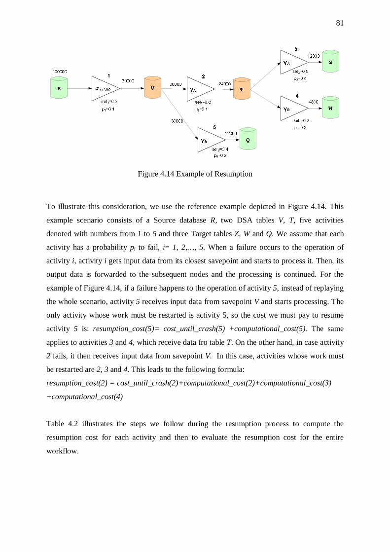
81

Figure 4.14 Example of Resumption

To illustrate this consideration, we use the reference example depicted in Figure 4.14. This

example scenario consists of a Source database R, two DSA tables V, T, five activities

denoted with numbers from 1 to 5 and three Target tables Z, W and Q. We assume that each

activity has a probability pi to fail, i= 1, 2,…, 5. When a failure occurs to the operation of

activity i, activity i gets input data from its closest savepoint and starts to process it. Then, its

output data is forwarded to the subsequent nodes and the processing is continued. For the

example of Figure 4.14, if a failure happens to the operation of activity 5, instead of replaying

the whole scenario, activity 5 receives input data from savepoint V and starts processing. The

only activity whose work must be restarted is activity 5, so the cost we must pay to resume

activity 5 is: resumption_cost(5)= cost_until_crash(5) +computational_cost(5). The same

applies to activities 3 and 4, which receive data fro table T. On the other hand, in case activity

2 fails, it then receives input data from savepoint V. In this case, activities whose work must

be restarted are 2, 3 and 4. This leads to the following formula:

resumption_cost(2) = cost_until_crash(2)+computational_cost(2)+computational_cost(3)

+computational_cost(4)

Table 4.2 illustrates the steps we follow during the resumption process to compute the

resumption cost for each activity and then to evaluate the resumption cost for the entire

workflow.

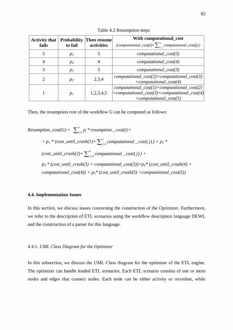
82

Table 4.2 Resumption steps

Activity that fails

Probability to fail

Then resume activities

With computational_cost

(computational_cost(i)+m

j=1computational_cost(j)∑ )

5 p5 5 computational_cost(5)

4 p4 4 computational_cost(4)

3 p3 3 computational_cost(3)

2 p2 2,3,4 computational_cost(2)+computational_cost(3)

+computational_cost(4)

1 p1 1,2,3,4,5 computational_cost(1)+computational_cost(2)

+computational_cost(3)+computational_cost(4) +computational_cost(5)

Then, the resumption cost of the workflow G can be computed as follows:

Resumption_cost(G) = 5

1_ii

p * resumption cost(i)=∑ =

= p1 * (cost_until_crash(1)+5

1_ ( )

jcomputational cost j

=∑ ) + p2 *

(cost_until_crash(2)+4

2_ ( )

jcomputational cost j

=∑ ) +

p3 * (cost_until_crash(3) + computational_cost(3))+p4* (cost_until_crash(4) +

computational_cost(4)) + p5* (cost_until_crash(5) +computational_cost(5))

4.4. Implementation Issues

In this section, we discuss issues concerning the construction of the Optimizer. Furthermore,

we refer to the description of ETL scenarios using the workflow description language DEWL

and the construction of a parser for this language.

4.4.1. UML Class Diagram for the Optimizer

In this subsection, we discuss the UML Class diagram for the optimizer of the ETL engine.

The optimizer can handle loaded ETL scenarios. Each ETL scenario consists of one or more

nodes and edges that connect nodes. Each node can be either activity or recordset, while

83

recordsets are further discriminated in tables or files. Figure 4.15 shows the UML Class

diagram for the optimizer.

We now analyze each component of the UML Class diagram.

1. The Scenario is set of data transformation processes that must be executed

sequentially. Each scenario is characterized by a name (ScenarioName) and contains

an activity list (ListOfActivities) and a recordset list (ListOfRecordsets). Both activities

and recordsets compose a list of graph nodes (ListOfNodes). Furthermore, there exists

a list of graph edges (ListOfEdges) and a list with the orders on each edge

(ListOfEdgeOrders). Each scenario has an operational cost (ScenarioCost) and a

unique signature (ScenarioSignature). The signature of a scenario is a string that

characterizes the scenario and is described in detail in section 4.1.4. The scenario also

contains the method ComputeScenarioCost() that computes the cost of the whole

scenario, by adding the costs of its activities and recordsets. The method

ComputeResumptionCost() computes the resumption cost and

ComputeScenarioSignature() evaluates the signature of the scenario.

2. Nodes are the component parts of an ETL scenario and are connected through the

graph Edges. Each node has a name to which someone can refer (NodeName) and a

cost that represents the cost to process the incoming data. The resumption cost for the

node is called Rescost. Each node has a number of nodes as inputs and a number of

nodes as outputs. The number of input tuples is called InputTuples.The methods

getCost() and getOutputSize() are used for the retrieval of the NodeCost and the node’s

OutputSize (i.e., number of output tuples) accordingly. On the other hand, the

methods ComputeCost(), ComputeResCost(), ComputeOutputSize() and

ComputeSignature() calculate the cost of the node, the resumption cost, its

outputSize and generate the signature accordingly. Each Edge has a name (EdgeName)

and connects two nodes (SourceNode and TargetNode). Moreover, each edge that was

part of the initial workflow is described as Original, while others are not Original

edges.

3. Tables are relational tables that play a part in the scenario and store the input and

output tuples of each activity. Each table has a name (TableName) and a type,

characterized by one of the keywords: SOURCE, DSA or TARGET. Furthermore,

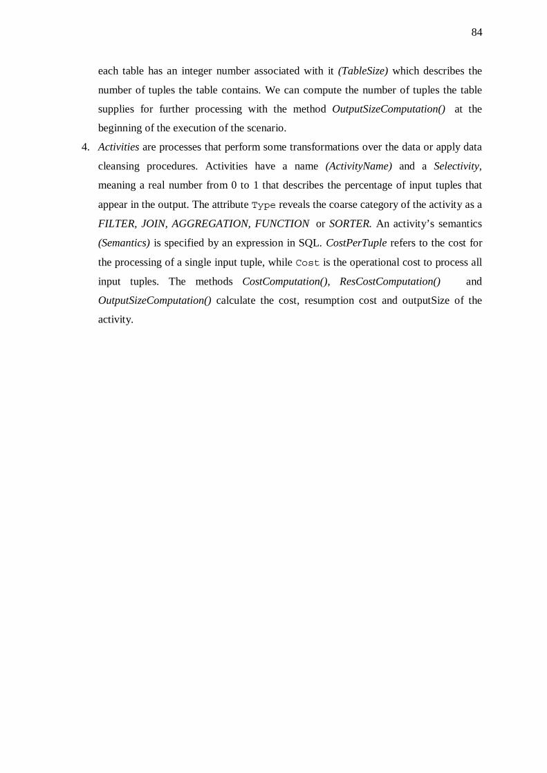
84

each table has an integer number associated with it (TableSize) which describes the

number of tuples the table contains. We can compute the number of tuples the table

supplies for further processing with the method OutputSizeComputation() at the

beginning of the execution of the scenario.

4. Activities are processes that perform some transformations over the data or apply data

cleansing procedures. Activities have a name (ActivityName) and a Selectivity,

meaning a real number from 0 to 1 that describes the percentage of input tuples that

appear in the output. The attribute Type reveals the coarse category of the activity as a

FILTER, JOIN, AGGREGATION, FUNCTION or SORTER. An activity’s semantics

(Semantics) is specified by an expression in SQL. CostPerTuple refers to the cost for

the processing of a single input tuple, while Cost is the operational cost to process all

input tuples. The methods CostComputation(), ResCostComputation() and

OutputSizeComputation() calculate the cost, resumption cost and outputSize of the

activity.

85

+New()

+ComputeScenarioCost()

+ComputeResumptionCost()

+ComputeScenarioSignature()

+ScenarioName : String

+ListOfActivities : myDictionary

+ListOfRecordsets : myDictionary

+ListOfNodes : myDictionary

+ListOfEdges : myDictionary

+ListOfEdgeOrders : myDictionary

+ScenarioCost : Double

+ScenarioSignature : String

Scenario

+New()

+EdgeName : String

+SourceNode : String

+TargetNode : String

+Original : Boolean

Edge

+New()

+getCost() : Double

+ComputeCost() : Double

+ComputeResCost() : Double

+getOutputSize() : Long

+ComputeOutputSize() : Long

+getSignature() : String+ComputeSignature() : String

+NodeName : String

+NodeCost : Double

+ResCost : Double

+Inputs : String

+Outputs : String

+InputTuples : Long+OutputSize : Long

Node1..*

+New()

+OutputSizeComputation() : Long

+TableName : String

+TableSize : Integer

Table

+New()

+CostComputation() : Double

+ResCostComputation() : Double

+OutputSizeComputation() : Long

+ActivityName : String

+Selectivity : Double

+Type : String

+Semantics : String

+CostPerTuple : Double

+Cost : Double

+Probability : Double

Activity

+New()

Filter

+New()

Filter_Greater

+New()

Filter_LowerEqual

+New()

Filter_Lower

+New()

Filter_GreaterEqual

+New()

Filter_Equal

+New()

Filter_NotEqual

+New()

+CostComputation() : Double

Sorter

+New()

+CostComputation() : Double

Join

+New()

+CostComputation() : Double

Aggregation

+New()

+CostComputation() : Double

Function_application

+New()

+main()

Optimizer

+New()

NotNull

1..*

1

0..*

Recordset

File

Figure 4.15 UML Class diagram for the ETL Scenario

86

5. The subclasses of the Activity class are: Filter, Join, Aggregation,

Function_application and Sorter. Most of them have a method CostComputation() to

compute their cost, except for Filter that uses the corresponding function of its super-

class Activity to compute their cost.

6. The Filter class is the super-class of Filter_Lower, Filter_LowerEqual,

Filter_Greater, Filter_GreaterEqual, Filter_Equal and Filter_NotEqual.

7. The Filter_Equal class is a super-class of the NotNull class.

4.4.2. Language DEWL for ETL Scenarios

Apart from the logical representation of an ETL scenario as a directed acyclic graph that we

discussed in previous sections, we have introduced a new language for the description of ETL

scenarios. We call this language DEWL (Data Exchange Workflow Language). DEWL is

simple and easy to write. DEWL is composed of four statements: the CREATE SCENARIO,

CREATE ACTIVITY, CREATE TABLE and the DECLARE INPUT OUTPUT statement.

1. The CREATE SCENARIO statement is used to define a new scenario. The user has to

provide the name of the scenario along with the names of the tables and the names of

the activities that compose the scenario.

2. The CREATE ACTIVITY statement defines an activity of the scenario. One has to

provide the name of the activity and its type, using one of the keywords: FILTER,

JOIN, AGGREGATION or FUNCTION. To this point, we have to make clear that sorter

activities cannot be part of the original scenario. This means that sorters cannot be

created through DEWL statements and the user cannot define any kinds of activities

other than filters, joins, aggregations or functions. Then the user provides a list of

parameters enclosed in parenthesis, which refers to the interesting orders for the

activity. In case the activity is a FILTER, one has to provide a comma delimited list

that contains the selection condition of the activity’s semantics. For example, for a

FILTER that expresses the selection σAGE>20 one has to provide the list (AGE,>,20). In

case the activity is a JOIN, one has to supply two lists of interesting orders, one for

each input of the activity, e.g., (ID;EMP_ID). The two lists of attributes are delimited

by a semicolon. For all other types of activities (aggregations, functions, etc.), one has

to provide one list of attributes that symbolize interesting orders, e.g., (ID,SAL).

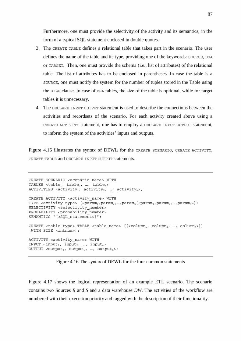
87

Furthermore, one must provide the selectivity of the activity and its semantics, in the

form of a typical SQL statement enclosed in double quotes.

3. The CREATE TABLE defines a relational table that takes part in the scenario. The user

defines the name of the table and its type, providing one of the keywords: SOURCE, DSA

or TARGET. Then, one must provide the schema (i.e., list of attributes) of the relational

table. The list of attributes has to be enclosed in parentheses. In case the table is a

SOURCE, one must notify the system for the number of tuples stored in the Table using

the SIZE clause. In case of DSA tables, the size of the table is optional, while for target

tables it is unnecessary.

4. The DECLARE INPUT OUTPUT statement is used to describe the connections between the

activities and recordsets of the scenario. For each activity created above using a

CREATE ACTIVITY statement, one has to employ a DECLARE INPUT OUTPUT statement,

to inform the system of the activities’ inputs and outputs.

Figure 4.16 illustrates the syntax of DEWL for the CREATE SCENARIO, CREATE ACTIVITY,

CREATE TABLE and DECLARE INPUT OUTPUT statements.

CREATE SCENARIO <scenario_name> WITH TABLES <table1, table2, …, tablem> ACTIVITIES <activity1, activity2, …, activityn>; CREATE ACTIVITY <activity_name> WITH TYPE <activity_type> (<param1,param2,…,paramm[;param1,param2,…,paramn>]) SELECTIVITY <selectivity_number> PROBABILITY <probability_number> SEMANTICS “[<SQL_statement>]”; CREATE <table_type> TABLE <table_name> [(<column1, column2, …, columnn>)] [WITH SIZE <intnum>]; ACTIVITY <activity_name> WITH INPUT <input1, input2, …, inputm> OUTPUT <output1, output2, …, outputn>;

Figure 4.16 The syntax of DEWL for the four common statements

Figure 4.17 shows the logical representation of an example ETL scenario. The scenario

contains two Sources R and S and a data warehouse DW. The activities of the workflow are

numbered with their execution priority and tagged with the description of their functionality.

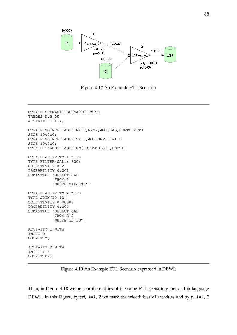
88

Figure 4.17 An Example ETL Scenario

CREATE SCENARIO SCENARIO1 WITH TABLES R,S,DW ACTIVITIES 1,2; CREATE SOURCE TABLE R(ID,NAME,AGE,SAL,DEPT) WITH SIZE 100000; CREATE SOURCE TABLE S(ID,AGE,DEPT) WITH SIZE 100000; CREATE TARGET TABLE DW(ID,NAME,AGE,DEPT); CREATE ACTIVITY 1 WITH TYPE FILTER(SAL,<,500) SELECTIVITY 0.2 PROBABILITY 0.001 SEMANTICS "SELECT SAL FROM R WHERE SAL<500"; CREATE ACTIVITY 2 WITH TYPE JOIN(ID;ID) SELECTIVITY 0.00005 PROBABILITY 0.004 SEMANTICS "SELECT SAL FROM R,S WHERE ID=ID"; ACTIVITY 1 WITH INPUT R OUTPUT 2; ACTIVITY 2 WITH INPUT 1,S OUTPUT DW;

Figure 4.18 An Example ETL Scenario expressed in DEWL

Then, in Figure 4.18 we present the entities of the same ETL scenario expressed in language

DEWL. In this Figure, by seli, i=1, 2 we mark the selectivities of activities and by pi, i=1, 2

89

their probabilities of failure. These probabilities are necessary for the calculation of the

resumption cost.

4.4.3. Parser

We mentioned in earlier sections that the ETL engine gets as input loaded ETL scenarios.

These scenarios are expressed in DEWL and stored at simple text files. In this work, we

decided to build a parser for our workflow definition language DEWL, because a parser can

be quite useful in programming tasks, such as reading source text files, extracting data from

formatted files, and verifying the correctness of data formats. For this reason, we

implemented a parser for the workflow definition language DEWL using the program

ProGrammar Parser Development Toolkit v1.20a by NorKen Technologies, Inc., a trial

version of which is available through the Internet ([PPDT06]). ProGrammar is a software tool

for Building, Testing and Debugging Parsers. ProGrammar is a visual development

environment that simplifies the process of building parsers. ProGrammar consists of the

following components:

Table 4.3 ProGrammar Components

Interactive Development Environment

Visual environment for building, testing and debugging parsers.

Grammar Definition Language

High-level notation used to express data syntax.

Parse Engine

Runtime component that parses input data. The parse engine is available as a Windows DLL, static library, and as an ActiveX control.

Application ProGrammar

Interface (API)

Programming interface for calling the parse engine at runtime.

One of the reasons it was selected for the development of a parser for DEWL, is the ease with

which ProGrammar can be integrated to Microsoft Visual Studio NET 2003. The parse

engine can be called from any development environment that supports ActiveX controls,

including Visual Basic NET. The only thing one has to do from the Visual Basic project is to

add a reference to the ProGrammar library PgmrX120Lib.dll located in the directory

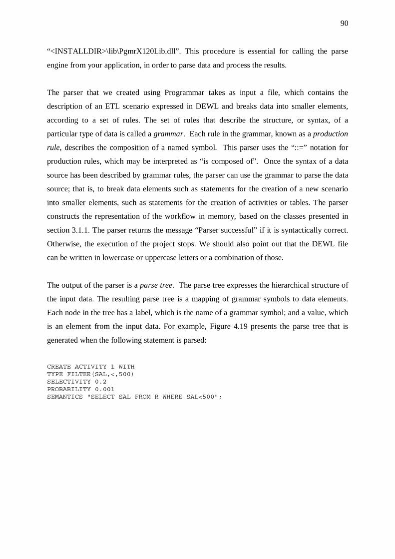
90

“<INSTALLDIR>\lib\PgmrX120Lib.dll”. This procedure is essential for calling the parse

engine from your application, in order to parse data and process the results.

The parser that we created using Programmar takes as input a file, which contains the

description of an ETL scenario expressed in DEWL and breaks data into smaller elements,

according to a set of rules. The set of rules that describe the structure, or syntax, of a

particular type of data is called a grammar. Each rule in the grammar, known as a production

rule, describes the composition of a named symbol. This parser uses the “::=” notation for

production rules, which may be interpreted as “is composed of”. Once the syntax of a data

source has been described by grammar rules, the parser can use the grammar to parse the data

source; that is, to break data elements such as statements for the creation of a new scenario

into smaller elements, such as statements for the creation of activities or tables. The parser

constructs the representation of the workflow in memory, based on the classes presented in

section 3.1.1. The parser returns the message “Parser successful” if it is syntactically correct.

Otherwise, the execution of the project stops. We should also point out that the DEWL file

can be written in lowercase or uppercase letters or a combination of those.

The output of the parser is a parse tree. The parse tree expresses the hierarchical structure of

the input data. The resulting parse tree is a mapping of grammar symbols to data elements.

Each node in the tree has a label, which is the name of a grammar symbol; and a value, which

is an element from the input data. For example, Figure 4.19 presents the parse tree that is

generated when the following statement is parsed:

CREATE ACTIVITY 1 WITH TYPE FILTER(SAL,<,500) SELECTIVITY 0.2 PROBABILITY 0.001 SEMANTICS "SELECT SAL FROM R WHERE SAL<500";

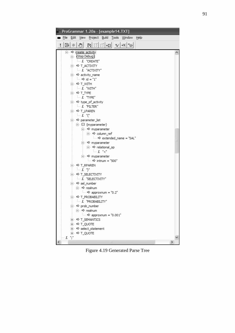
91

Figure 4.19 Generated Parse Tree

92

4.4.4. Parameters of the Algorithm GPO

We mentioned in section 4.2.2 that in order for the algorithm GPO to work for black box

activities, the designer of the workflow needs to specify a set of parameters.

1. FILTERS:

We assume that filters contain simple selection conditions of the form: <Attribute>

<Relational operator> <Value>, e.g., age>20. More composite filters can be created by

creating more than one activities that filter tuples. For example, a selection condition of the

form age >20 and salary<2000 can be expressed by creating two filters: one having

AGE>20 as its selection condition and another with the condition salary<2000. To construct

a filter, the designer supplies the parameters of the selection condition. The first parameter is

considered as the interesting order for the filter. Thus, in our setting, filters have only one

interesting order. For example, for a filter with condition age >20, the designer supplies the

parameter list age,>,20 and only the attribute age is the interesting order.

2. JOINS:

In case the activity is a join of tables A and B, one has to supply two lists of parameters, i.e.,

interesting orders, one (id; emp_id). for each input of the activity. The two lists of attributes

are delimited by a semicolon, e.g., Both parameters correspond to the attributes that

participate in the join of the tables. In our example, the join condition for the join of the tables

A and B is A.id = B. emp_id. The designer supplies the list (id; emp_id).

3. AGGREGATIONS:

The designer supplies the grouping attributes in a comma delimited list of parameters. For

example, for an activity γdept,age of type aggregation the designer provides the list of interesting

orders: (dept, age). All the parameters in the list are considered interesting orders.

4. FUNCTIONS:

For functions, one has to provide one list of attributes that symbolize interesting orders, e.g.,

(id, age).

Tables 4.4 to 4.7 summarize the aforementioned considerations for the interesting orders of

each activity class.

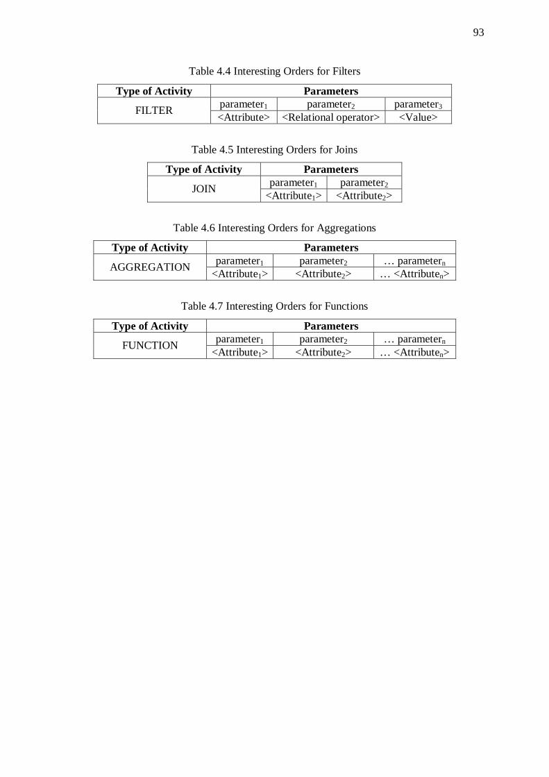
93

Table 4.4 Interesting Orders for Filters

Type of Activity Parameters parameter1 parameter2 parameter3 FILTER <Attribute> <Relational operator> <Value>

Table 4.5 Interesting Orders for Joins

Type of Activity Parameters parameter1 parameter2 JOIN

<Attribute1> <Attribute2>

Table 4.6 Interesting Orders for Aggregations

Type of Activity Parameters parameter1 parameter2 … parametern AGGREGATION

<Attribute1> <Attribute2> … <Attributen>

Table 4.7 Interesting Orders for Functions

Type of Activity Parameters parameter1 parameter2 … parametern FUNCTION

<Attribute1> <Attribute2> … <Attributen>

94

CHAPTER 5. EXPERIMENTS

5.1 Categories of Workflows

5.2 Experiments for Regular Operation with Recovery from Failures

5.3 Linear Workflows

5.4 Wishbones

5.5 Primary Flows

5.6 Trees

5.7 Forks

5.8 Butterflies

5.9 Observations Deduced from Experiments

In this Chapter, we experimentally assess the proposed approach using different classes of

workflows. We present a number of experiments that we have conducted to support the

conclusions of our theoretical work and to demonstrate the quality and the efficiency of the

proposed method. We tested the exhaustive algorithm on several classes of workflows by

making variations over different measures, such as:

• the size of the workflow (i.e., the number of nodes contained in the graph),

• the size of data originating from the sources,

• the selectivities of the activities of the workflow

• the values of probabilities of failure, etc.

For each set of experiments, we recorded certain measures, such as:

• Completion time: Time needed by the exhaustive algorithm to discover the optimal

physical-level scenario.

95

• Number of generated signatures: The number of generated signatures corresponds to

the number of the physical-level scenarios created by exploring all the alternative

combinations of physical-level activities, along with the possible addition of one or

more sorters to the original logical-level scenario.

• Computational Cost: Cost for processing of source data, assuming that all activities

complete their regular operation successfully (i.e., the system works without failures).

• Resumption Cost: Cost to restart processing of data due to failures in the operation of

the activities of the workflow.

• Total Cost: The sum of the operational cost of the scenario and the resumption cost.

• Number of sorters: The number of sorters contained in a signature (i.e., a physical

representation of the scenario).

• Cost of Sorters: The additional cost for the system caused by the introduction of sorter

activities to the scenario. This cost is computed by adding the cost of all sorters

contained in a workflow.

• Percentage of Sorter Cost: The percentage of the cost of sorters with respect to the

total cost of the workflow. This percentage for a state i is computed as follows:

Cost of Sorters(i) Percentage of Sorter Cost(i) =

Total Cost(i)

All the experiments were conducted on an Intel(R) Pentium(R) M machine running at 1,86

GHz with 1 GB RAM.

5.1. Categories of Workflows

In this work, we have set up a series of experiments for various types of workflows. We

classify workflows according to their node structure. To this point, we introduce a broad

category of workflows, called Butterflies. A butterfly is an ETL workflow that consists of

three distinct components: (a) the left wing, (b) the body and (c) the right wing of the

butterfly. The left and right wings are two non-overlapping groups of nodes which are

attached to the body of the butterfly. The three parts of the butterfly are presented in more

detail as follows:

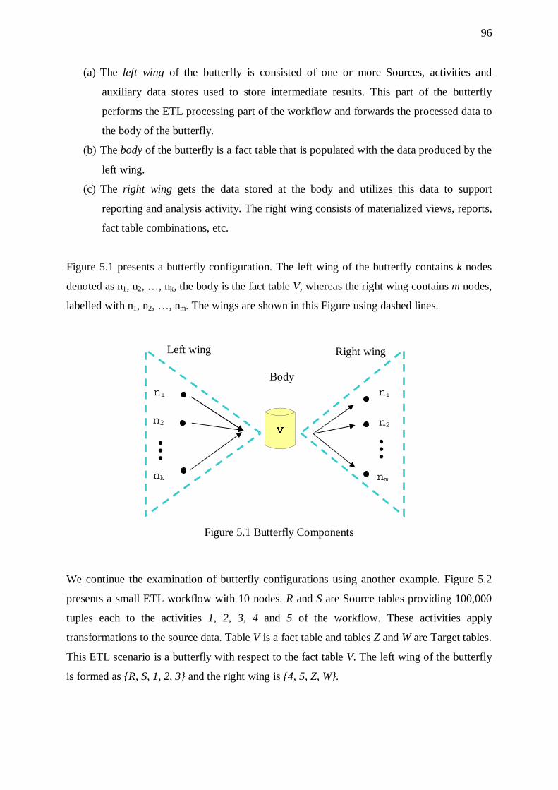
96

(a) The left wing of the butterfly is consisted of one or more Sources, activities and

auxiliary data stores used to store intermediate results. This part of the butterfly

performs the ETL processing part of the workflow and forwards the processed data to

the body of the butterfly.

(b) The body of the butterfly is a fact table that is populated with the data produced by the

left wing.

(c) The right wing gets the data stored at the body and utilizes this data to support

reporting and analysis activity. The right wing consists of materialized views, reports,

fact table combinations, etc.

Figure 5.1 presents a butterfly configuration. The left wing of the butterfly contains k nodes

denoted as n1, n2, …, nk, the body is the fact table V, whereas the right wing contains m nodes,

labelled with n1, n2, …, nm. The wings are shown in this Figure using dashed lines.

Figure 5.1 Butterfly Components

We continue the examination of butterfly configurations using another example. Figure 5.2

presents a small ETL workflow with 10 nodes. R and S are Source tables providing 100,000

tuples each to the activities 1, 2, 3, 4 and 5 of the workflow. These activities apply

transformations to the source data. Table V is a fact table and tables Z and W are Target tables.

This ETL scenario is a butterfly with respect to the fact table V. The left wing of the butterfly

is formed as R, S, 1, 2, 3 and the right wing is 4, 5, Z, W.

Body

Right wing Left wing

n1

n2

nm

n1

n2

nk

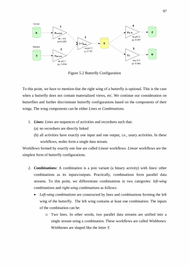
97

Figure 5.2 Butterfly Configuration

To this point, we have to mention that the right wing of a butterfly is optional. This is the case

when a butterfly does not contain materialized views, etc. We continue our consideration on

butterflies and further discriminate butterfly configurations based on the components of their

wings. The wing components can be either Lines or Combinations.

1. Lines: Lines are sequences of activities and recordsets such that:

(a) no recordsets are directly linked

(b) all activities have exactly one input and one output, i.e., unary activities. In these

workflows, nodes form a single data stream.

Workflows formed by exactly one line are called Linear workflows. Linear workflows are the

simplest form of butterfly configurations.

2. Combinations: A combination is a join variant (a binary activity) with lines/ other

combinations as its inputs/outputs. Practically, combinations form parallel data

streams. To this point, we differentiate combinations in two categories: left-wing

combinations and right-wing combinations as follows:

• Left-wing combinations are constructed by lines and combinations forming the left

wing of the butterfly. The left wing contains at least one combination. The inputs

of the combination can be:

o Two lines. In other words, two parallel data streams are unified into a

single stream using a combination. These workflows are called Wishbones.

Wishbones are shaped like the letter Y.

98

o A line and a recordset. The primary flow of data is the line part of the

workflow. The line and a Look-up table are joined into a single stream by

the combination.

o Two or more combinations. The use of combinations leads to many parallel

data streams. These workflows are called Trees.

• Right-wing combinations are constructed by lines and combinations on the right

wing of the butterfly. These lines and combinations form either a flat or a deep

hierarchy. These hierarchies are explained next:

o Flat Hierarchies: These configurations have small depth (exactly 2) and

large fan-out. By depth, we mean the number of nodes (activities or

recordsets) in the longest path from the body of the butterfly to the target

table(s). We assume zero depth for the body and measure depth

incrementally as we follow the stream towards the targets. By fan-out we

refer to the number of outputs of the body of the butterfly, i.e., to the

number of streams generated by the body. An example of such a workflow

is a Fork, where a single data stream is split in two or more parallel data

streams. The split is performed with the assistance of a fact table (the body)

that forwards its data in two or more activities.

o Right - Deep Hierarchies: These configurations have depth more than 4

and medium fan-out. Figure 5.3 (f) shows a right - deep hierarchy with

depth 6.

Figure 5.3 shows examples of the aforementioned special butterfly configurations. Observe

that the sources and the warehouse are depicted with simple lines in their borders, whereas the

bodies of the butterflies are depicted in thicker border. In the cases of trees and primary flows,

the target warehouse acts as the body of the butterfly (i.e., there is no right wing). We can

construct more complex butterfly structures by combining some of the above configurations.

In the following sections, we will present the experiments we conducted using special

categories of butterfly configurations, i.e., Linear Workflows, Forks, Wishbones, Trees, etc.

5.2. Experiments for Regular Operation with Recovery from Failures

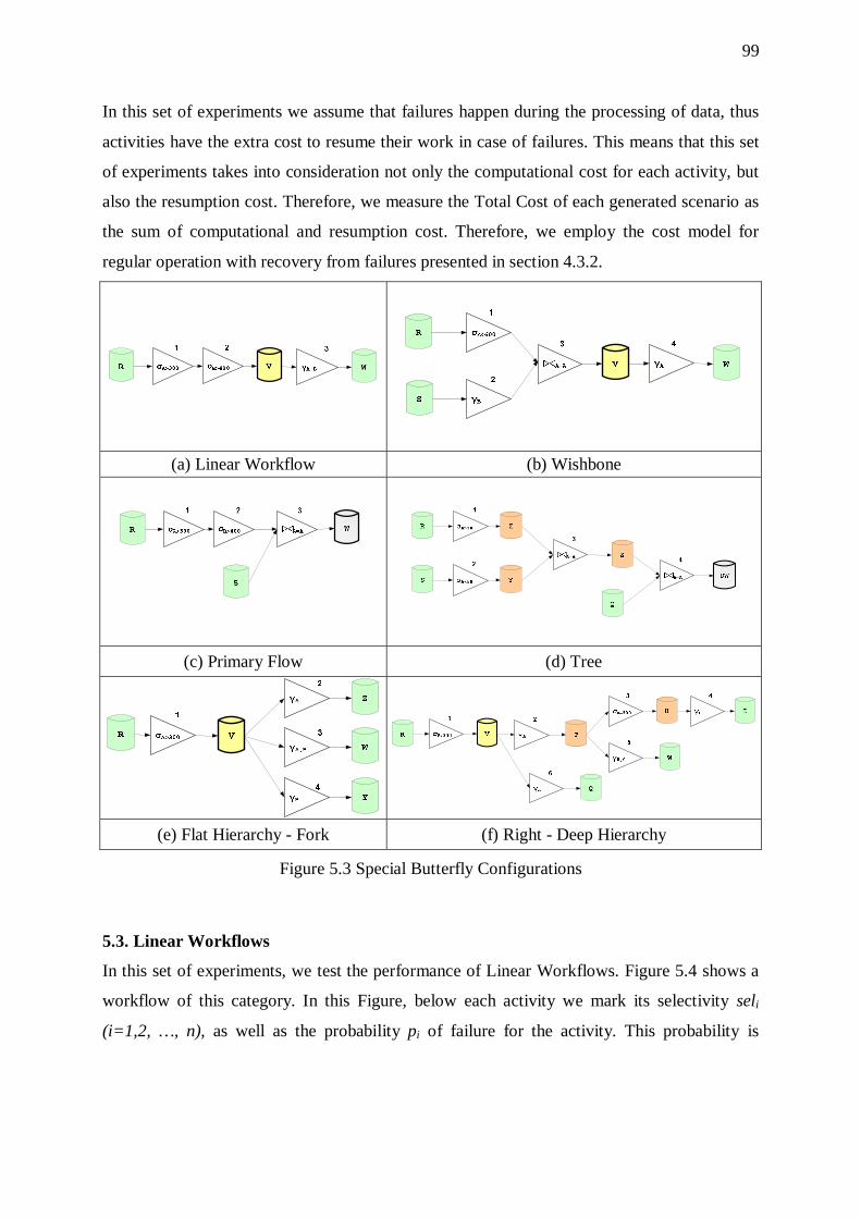
99

In this set of experiments we assume that failures happen during the processing of data, thus

activities have the extra cost to resume their work in case of failures. This means that this set

of experiments takes into consideration not only the computational cost for each activity, but

also the resumption cost. Therefore, we measure the Total Cost of each generated scenario as

the sum of computational and resumption cost. Therefore, we employ the cost model for

regular operation with recovery from failures presented in section 4.3.2.

(a) Linear Workflow (b) Wishbone

(c) Primary Flow (d) Tree

γA

2

V

Z

σA>300

1

γA,Β

3

W

γB

4

Y

R

(e) Flat Hierarchy - Fork (f) Right - Deep Hierarchy

Figure 5.3 Special Butterfly Configurations

5.3. Linear Workflows

In this set of experiments, we test the performance of Linear Workflows. Figure 5.4 shows a

workflow of this category. In this Figure, below each activity we mark its selectivity seli

(i=1,2, …, n), as well as the probability pi of failure for the activity. This probability is

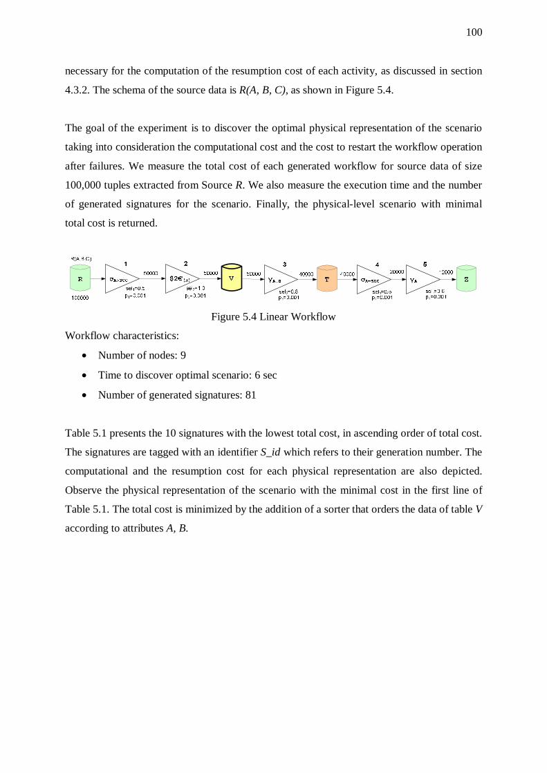
100

necessary for the computation of the resumption cost of each activity, as discussed in section

4.3.2. The schema of the source data is R(A, B, C), as shown in Figure 5.4.

The goal of the experiment is to discover the optimal physical representation of the scenario

taking into consideration the computational cost and the cost to restart the workflow operation

after failures. We measure the total cost of each generated workflow for source data of size

100,000 tuples extracted from Source R. We also measure the execution time and the number

of generated signatures for the scenario. Finally, the physical-level scenario with minimal

total cost is returned.

Figure 5.4 Linear Workflow

Workflow characteristics:

• Number of nodes: 9

• Time to discover optimal scenario: 6 sec

• Number of generated signatures: 81

Table 5.1 presents the 10 signatures with the lowest total cost, in ascending order of total cost.

The signatures are tagged with an identifier S_id which refers to their generation number. The

computational and the resumption cost for each physical representation are also depicted.

Observe the physical representation of the scenario with the minimal cost in the first line of

Table 5.1. The total cost is minimized by the addition of a sorter that orders the data of table V

according to attributes A, B.

101

Table 5.1 Top-10 Signatures for Linear Workflow

S_id Top-10 Signatures Computational Cost

Resumption Cost Total Cost

6 R.1.2.V.V!(A,B).3@SO.T.4.5@SO.Z 1.040.482 880 1.041.362 2 R.1.2.V.3@SO.T.4.5@SO.Z 1.040.482 3.612 1.044.094 28 R.1.2.V.V!(A,B).3@SO.T.4.4_5(A).5@SO.Z 1.346.236 860 1.347.096 10 R.1.2.V.3@SO.T.4.4_5(A).5@SO.Z 1.346.236 3.592 1.349.828 20 R.1.2.V.V!(A,B).3@SO.T.T!(A).4.5@SO.Z 1.651.991 880 1.652.871 8 R.1.2.V.3@SO.T.T!(A).4.5@SO.Z 1.651.991 3.612 1.655.602 4 R.1.2.V.V!(A).3@SO.T.4.5@SO.Z 1.820.964 3.612 1.824.576 5 R.1.2.V.V!(B).3@SO.T.4.5@SO.Z 1.820.964 3.612 1.824.576 7 R.1.2.V.V!(B,A).3@SO.T.4.5@SO.Z 1.820.964 3.612 1.824.576 24 R.1.1_2(B).2.V.V!(A,B).3@SO.T.4.5@SO.Z 1.870.964 780 1.871.744

In the sequel, we use the scenario of Figure 5.4 as a reference example and vary the size of the

input data, the volume of data pushed towards the warehouse and the graph size to assess their

impact over the completion time of the algorithm and the sensitivity of the top-10 solutions.

For the latter metric, we examine the effects of these factors to the top-10 solutions and to the

average of the top-10 solutions. Before proceeding, though, on these issues, we start with an

assessment of the role of the introduction of sorters to the scenario.

5.3.1. Overhead of Sorters

Table 5.2 presents the number of sorters contained in each of the aforementioned top-10

signatures, the sorters’ cost, and the percentage of this cost over the total cost of the scenario.

Table 5.2 Sorter Cost for Linear Workflow

S_id Number of Sorters

Cost of Sorters

Percentage of Sorter Cost

6 1 780.482 75% 2 0 0 0% 28 2 1.086.236 81% 10 1 305.754 23% 20 2 1.391.991 84% 8 1 611.508 37% 4 1 780.482 43% 5 1 780.482 43% 7 1 780.482 43% 24 2 1.610.964 86%

Observe that the overheads incurred by the introduction of sorters are quite significant in

several cases (in fact, the best and the third best solution have a quite high percentage of

102

sorter cost). In other words, the introduction of sorters minimizes the cost of the rest of the

activities so much, that the combination of activity and sorter costs ends up lower than (or

quite close to) the cost of the best possible configuration without any sorters (S_id = 2). In the

cases where the resumption cost has an upper threshold (i.e., the problem is stated as “find the

optimal configuration while guaranteeing that the resumption cost does not exceed a certain

threshold”), then the solutions with sorters are clearly the winners (see the resumption costs in

Table 5.1).

5.3.2. Effect of Input Size

The size of source R in the reference scenario of Figure 5.4 is 100,000 rows. We have also

experimented by varying the size of source data as 50,000, 150,000 and 200,000 rows. All

experiments return the same top-10 solutions. We have also observed that the total cost of the

optimal solution in all cases is practically linearly dependent upon the input size. This

observation holds also for the average cost of the top-10 signatures and the 10th solution.

5.3.3. Effect of the Overall Selectivity of the Workflow

In the experiments of this paragraph, we modify the selectivity values of the workflow in such

a way, that small, medium or large volumes of data reach the output. In particular, we

appropriately tune the selectivities, so that the ratio of the output data over the input data is:

0.1, 0.3, 0.5 or 0.7. In other words, we try to assess the impact of the overall selectivity of the

workflow to the overall cost.

Table 5.3 Effect of Data Volume propagated towards the Warehouse

0.1|R| 0.3|R| 0.5|R| 0.7|R| # of different solutions in

top-10 list 0 0 0 0

Change at Optimal Solution No No No No

Total cost (Optimal) 1.041.362 1.718.192 1.538.360 1.981.880

Total cost (Avg(Top-10)) 1.543.632 2.624.910 2.389.660 3.100.692

Total cost(10th) 1.871.744 3.101.109 2.734.915 3.552.968

Optimal 0 676.830 496.998 940.518

Avg(Top-10) 0 1.081.277 846.028 1.557.060 Difference in total cost

10th 0 1.229.365 863.171 1.681.224

Optimal 0 65% 48% 90%

Avg(Top-10) 0 70% 55% 101% Difference in total cost

(%) 10th 0 66% 46% 90%

103

In the reference example of Figure 5.4, we notice that the ratio of output data over input data

is approximately 0.1. We compare the top-10 signatures for all the variants of the reference

scenario and measure the following metrics:

- The number of different signatures in the top-10 list.

- The existence of a change at the optimal (top-1) solution.

- The absolute costs for (a) the optimal solution, (b) the average cost of the top-10

signatures and (c) the 10th solution.

- The difference in total cost of the aforementioned 3 solutions compared to the

corresponding values of the reference example.

- The above difference as a percentage.

Table 5.3 depicts the measurements for the above metrics when the ratio of output data over

input data is 0.1, 0.3, 0.5 and 0.7.

Notice that the top-10 solutions remain the same, irrespectively of the data volumes that reach

the data warehouse. This means that linear workflows are quite reliable to the case of wrong

selectivity estimation.

In addition, observe that the relationship of the overall workflow selectivity and total cost is

not linear: in fact, the total cost drops for all the top-10 solutions for the case of 0.5|R|. This is

shown more clearly in the diagram of Figure 5.5, where the total cost values for the (a)

optimal solution, (b) the average of the top-10 signatures and (c) the 10th solution are

depicted. This relationship is not linear due to the fact that the total cost depends on the

volume of data that have to be ordered by the sorter of table V. In the case of 0.5|R|, the

selectivity of the first filter is higher than the one of the case of 0.3|R|. This means that (a) the

cost of the left wing of the line is lower for the case of 0.5|R| and (b) that the sorter applied

over the butterfly’s body V is also lower. Therefore, the lessons taught out of this experiment

lie in the role of the left wing as a filter: the more selective the left wing is, the higher the

possibility of exploiting sorters efficiently to speed up the operation of the right wing.

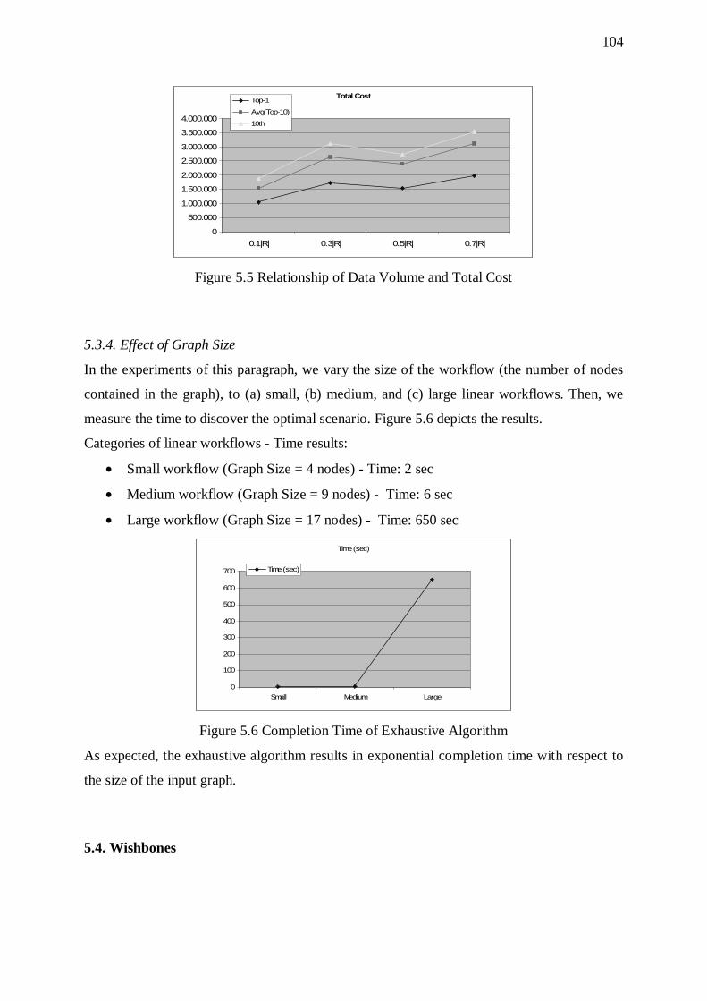
104

Total Cost

0

500.000

1.000.000

1.500.000

2.000.000

2.500.000

3.000.000

3.500.000

4.000.000

0.1|R| 0.3|R| 0.5|R| 0.7|R|

Top-1

Avg(Top-10)

10th

Figure 5.5 Relationship of Data Volume and Total Cost

5.3.4. Effect of Graph Size

In the experiments of this paragraph, we vary the size of the workflow (the number of nodes

contained in the graph), to (a) small, (b) medium, and (c) large linear workflows. Then, we

measure the time to discover the optimal scenario. Figure 5.6 depicts the results.

Categories of linear workflows - Time results:

• Small workflow (Graph Size = 4 nodes) - Time: 2 sec

• Medium workflow (Graph Size = 9 nodes) - Time: 6 sec

• Large workflow (Graph Size = 17 nodes) - Time: 650 sec

Time (sec)

0

100

200

300

400

500

600

700

Small Medium Large

Time (sec)

Figure 5.6 Completion Time of Exhaustive Algorithm

As expected, the exhaustive algorithm results in exponential completion time with respect to

the size of the input graph.

5.4. Wishbones

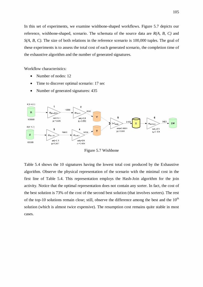
105

In this set of experiments, we examine wishbone-shaped workflows. Figure 5.7 depicts our

reference, wishbone-shaped, scenario. The schemata of the source data are R(A, B, C) and

S(A, B, C). The size of both relations in the reference scenario is 100,000 tuples. The goal of

these experiments is to assess the total cost of each generated scenario, the completion time of

the exhaustive algorithm and the number of generated signatures.

Workflow characteristics:

• Number of nodes: 12

• Time to discover optimal scenario: 17 sec

• Number of generated signatures: 435

Figure 5.7 Wishbone

Table 5.4 shows the 10 signatures having the lowest total cost produced by the Exhaustive

algorithm. Observe the physical representation of the scenario with the minimal cost in the

first line of Table 5.4. This representation employs the Hash-Join algorithm for the join

activity. Notice that the optimal representation does not contain any sorter. In fact, the cost of

the best solution is 73% of the cost of the second best solution (that involves sorters). The rest

of the top-10 solutions remain close; still, observe the difference among the best and the 10th

solution (which is almost twice expensive). The resumption cost remains quite stable in most

cases.

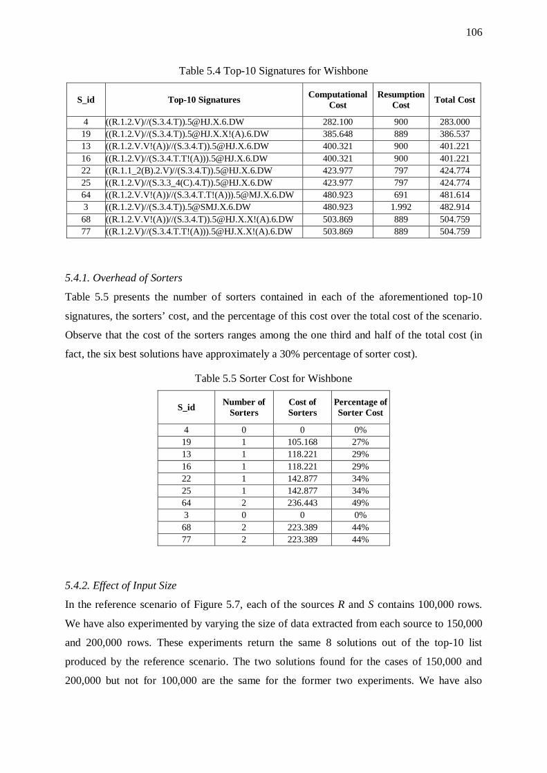
106

Table 5.4 Top-10 Signatures for Wishbone

S_id Top-10 Signatures Computational Cost

Resumption Cost Total Cost

4 ((R.1.2.V)//(S.3.4.T)).5@HJ.X.6.DW 282.100 900 283.000 19 ((R.1.2.V)//(S.3.4.T)).5@HJ.X.X!(A).6.DW 385.648 889 386.537 13 ((R.1.2.V.V!(A))//(S.3.4.T)).5@HJ.X.6.DW 400.321 900 401.221 16 ((R.1.2.V)//(S.3.4.T.T!(A))).5@HJ.X.6.DW 400.321 900 401.221 22 ((R.1.1_2(B).2.V)//(S.3.4.T)).5@HJ.X.6.DW 423.977 797 424.774 25 ((R.1.2.V)//(S.3.3_4(C).4.T)).5@HJ.X.6.DW 423.977 797 424.774 64 ((R.1.2.V.V!(A))//(S.3.4.T.T!(A))).5@MJ.X.6.DW 480.923 691 481.614 3 ((R.1.2.V)//(S.3.4.T)).5@SMJ.X.6.DW 480.923 1.992 482.914 68 ((R.1.2.V.V!(A))//(S.3.4.T)).5@HJ.X.X!(A).6.DW 503.869 889 504.759 77 ((R.1.2.V)//(S.3.4.T.T!(A))).5@HJ.X.X!(A).6.DW 503.869 889 504.759

5.4.1. Overhead of Sorters

Table 5.5 presents the number of sorters contained in each of the aforementioned top-10

signatures, the sorters’ cost, and the percentage of this cost over the total cost of the scenario.

Observe that the cost of the sorters ranges among the one third and half of the total cost (in

fact, the six best solutions have approximately a 30% percentage of sorter cost).

Table 5.5 Sorter Cost for Wishbone

S_id Number of Sorters

Cost of Sorters

Percentage of Sorter Cost

4 0 0 0% 19 1 105.168 27% 13 1 118.221 29% 16 1 118.221 29% 22 1 142.877 34% 25 1 142.877 34% 64 2 236.443 49% 3 0 0 0% 68 2 223.389 44% 77 2 223.389 44%

5.4.2. Effect of Input Size

In the reference scenario of Figure 5.7, each of the sources R and S contains 100,000 rows.

We have also experimented by varying the size of data extracted from each source to 150,000

and 200,000 rows. These experiments return the same 8 solutions out of the top-10 list

produced by the reference scenario. The two solutions found for the cases of 150,000 and

200,000 but not for 100,000 are the same for the former two experiments. We have also

107

observed that the total cost of the optimal solution in all cases is practically linearly dependent

upon the input size. This observation holds also for the average cost of the top-10 signatures

and the 10th solution.

5.4.3. Effect of the Overall Selectivity of the Workflow

In the experiments of this paragraph, we modify the selectivity of the wishbone’s join in such

a way, that small, medium or large volumes of data reach the output. The selectivity values

were tuned to the following values: |OuterRelation|-1, 5 ∗ |OuterRelation|-1, 10 ∗

|OuterRelation|-1. We have chosen these values to simulate the following possibilities: (a) for

each tuple of the inner relation R, exactly one tuple of the outer relation is matched (a.k.a. 1:1

join in the database literature), (b) for each tuple of the inner relation R, there are several

tuples (in our experiments: 5 or 10) of the outer relation matched on average (a.k.a. 1:N join

in the database literature). Since the latter is a rather high value for typical join situations, the

last experiment simulates the possibility of a N:M join, where the mappings of tuples of the

two relations are many to many.

Table 5.6 Effect of Data Volume propagated towards the Warehouse

1/|OUTER

RELATION| 5/|OUTER

RELATION| 10/|OUTER RELATION|

# of different solutions in top-10 list

0 3 3

Change at Optimal Solution No No No

Total cost (Optimal) 283.000 315.610 356.374

Total cost (Avg(Top-10)) 429.557 481.801 520.934

Total cost(10th) 504.759 575.606 616.370

Optimal 0 32.611 73.374

Avg(Top-10) 0 52.244 91.377 Difference in total cost

10th 0 70.848 111.611

Optimal 0 12% 26%

Avg(Top-10) 0 12% 21% Difference in total cost

(%) 10th 0 14% 22%

Observe that the optimal solution remains the same, irrespectively of the data volumes that are

propagated to the warehouse. As the volume of data is increased, only 3 out of the top-10

solutions are different. Furthermore, observe that the relationship of join selectivity and total

cost is linear: the total cost rises for all the top-10 solutions for larger data volumes. This is

shown more clearly in the diagram of Figure 5.8, where the total cost values for the (a)

108

optimal solution, (b) the average of the top-10 signatures and (c) the 10th solution are

depicted.

Total Cost

0

100.000

200.000

300.000

400.000

500.000

600.000

700.000

1 / |OUTERRELATION|

5 / |OUTERRELATION|

10 / |OUTERRELATION|

Top-1

Avg(Top-10)

10th

Figure 5.8 Relationship of Join Selectivity and Total Cost

5.4.4. Effect of Graph Size

In the experiments of this paragraph, we vary the size of the workflow (the number of nodes

contained in the graph), to (a) small, (b) medium, and (c) large wishbones. Then, we measure

the time to discover the optimal scenario. The specific values for the three variants of the

workflow are as follows:

• Small workflow (Graph Size = 8 nodes) - Time: 6 sec

• Medium workflow (Graph Size = 12 nodes) - Time: 17 sec

• Large workflow (Graph Size = 15 nodes) - Time: 1487 sec

Figure 5.9 depicts the results.

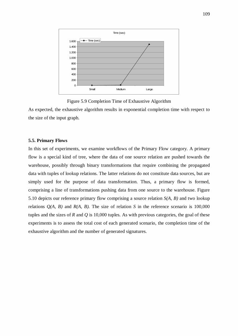
109

Time (sec)

0

200

400

600

800

1.000

1.200

1.400

1.600

Small Medium Large

Time (sec)

Figure 5.9 Completion Time of Exhaustive Algorithm

As expected, the exhaustive algorithm results in exponential completion time with respect to

the size of the input graph.

5.5. Primary Flows

In this set of experiments, we examine workflows of the Primary Flow category. A primary

flow is a special kind of tree, where the data of one source relation are pushed towards the

warehouse, possibly through binary transformations that require combining the propagated

data with tuples of lookup relations. The latter relations do not constitute data sources, but are

simply used for the purpose of data transformation. Thus, a primary flow is formed,

comprising a line of transformations pushing data from one source to the warehouse. Figure

5.10 depicts our reference primary flow comprising a source relation S(A, B) and two lookup

relations Q(A, B) and R(A, B). The size of relation S in the reference scenario is 100,000

tuples and the sizes of R and Q is 10,000 tuples. As with previous categories, the goal of these

experiments is to assess the total cost of each generated scenario, the completion time of the

exhaustive algorithm and the number of generated signatures.

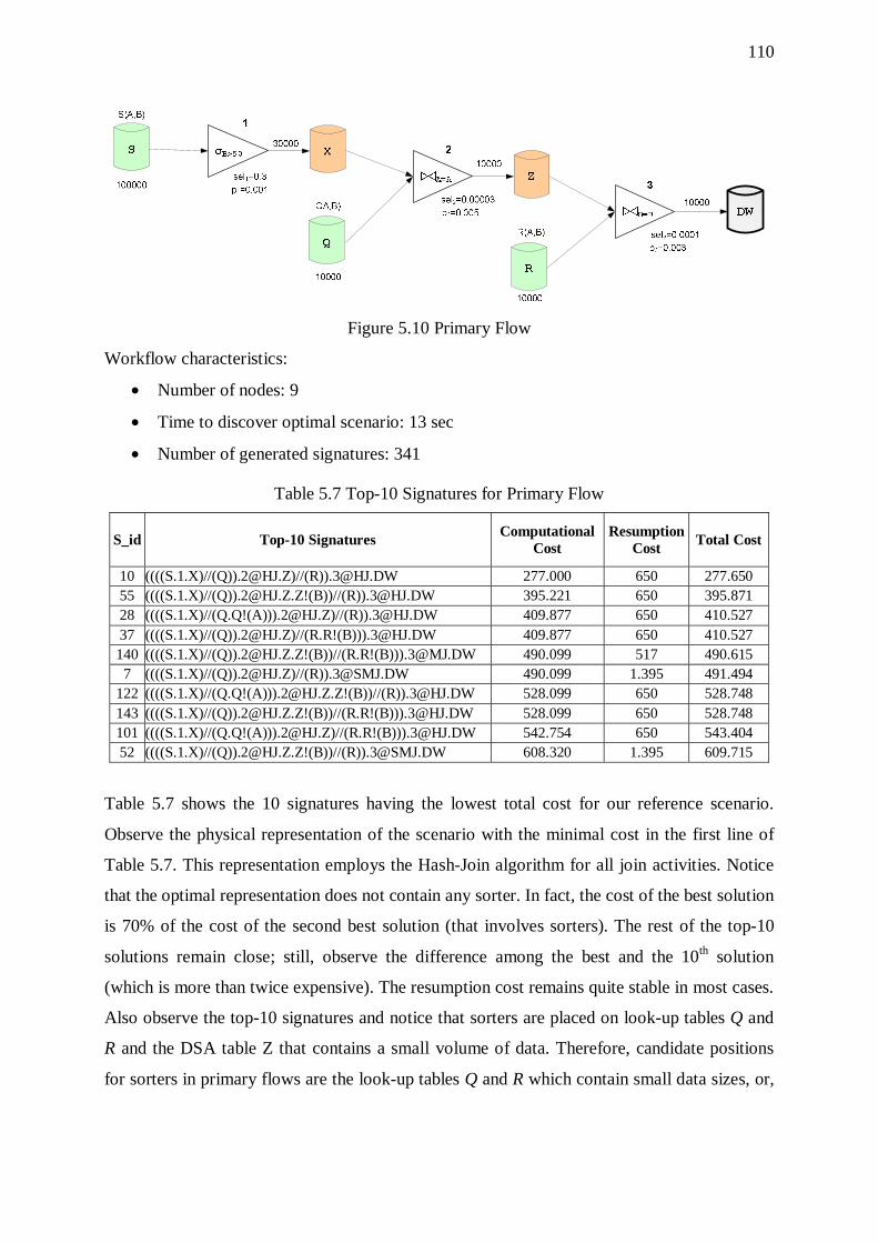
110

Figure 5.10 Primary Flow

Workflow characteristics:

• Number of nodes: 9

• Time to discover optimal scenario: 13 sec

• Number of generated signatures: 341

Table 5.7 Top-10 Signatures for Primary Flow

S_id Top-10 Signatures Computational Cost

Resumption Cost Total Cost

10 ((((S.1.X)//(Q)).2@HJ.Z)//(R)).3@HJ.DW 277.000 650 277.650 55 ((((S.1.X)//(Q)).2@HJ.Z.Z!(B))//(R)).3@HJ.DW 395.221 650 395.871 28 ((((S.1.X)//(Q.Q!(A))).2@HJ.Z)//(R)).3@HJ.DW 409.877 650 410.527 37 ((((S.1.X)//(Q)).2@HJ.Z)//(R.R!(B))).3@HJ.DW 409.877 650 410.527 140 ((((S.1.X)//(Q)).2@HJ.Z.Z!(B))//(R.R!(B))).3@MJ.DW 490.099 517 490.615

7 ((((S.1.X)//(Q)).2@HJ.Z)//(R)).3@SMJ.DW 490.099 1.395 491.494 122 ((((S.1.X)//(Q.Q!(A))).2@HJ.Z.Z!(B))//(R)).3@HJ.DW 528.099 650 528.748 143 ((((S.1.X)//(Q)).2@HJ.Z.Z!(B))//(R.R!(B))).3@HJ.DW 528.099 650 528.748 101 ((((S.1.X)//(Q.Q!(A))).2@HJ.Z)//(R.R!(B))).3@HJ.DW 542.754 650 543.404 52 ((((S.1.X)//(Q)).2@HJ.Z.Z!(B))//(R)).3@SMJ.DW 608.320 1.395 609.715

Table 5.7 shows the 10 signatures having the lowest total cost for our reference scenario.

Observe the physical representation of the scenario with the minimal cost in the first line of

Table 5.7. This representation employs the Hash-Join algorithm for all join activities. Notice

that the optimal representation does not contain any sorter. In fact, the cost of the best solution

is 70% of the cost of the second best solution (that involves sorters). The rest of the top-10

solutions remain close; still, observe the difference among the best and the 10th solution

(which is more than twice expensive). The resumption cost remains quite stable in most cases.

Also observe the top-10 signatures and notice that sorters are placed on look-up tables Q and

R and the DSA table Z that contains a small volume of data. Therefore, candidate positions

for sorters in primary flows are the look-up tables Q and R which contain small data sizes, or,

111

it is highly recommendable that these relations are already sorted before the execution of the

scenario. All other positions are not appropriate for sorters, due to the large number of join

activities, which produce large volumes of data to primary flows.

5.5.1. Overhead of Sorters

Table 5.8 presents the number of sorters contained in each of the top-10 signatures, the

sorters’ cost, and the percentage of this cost. Observe that the cost of the sorters ranges among

the one fifth and half of the total cost (in fact, the four best solutions have approximately a

30% percentage of sorter cost).

Table 5.8 Sorter Cost for Primary Flow

S_id Number of Sorters

Cost of Sorters

Percentage of Sorter Cost

10 0 0 0% 55 1 118.221 30% 28 1 132.877 32% 37 1 132.877 32%

140 2 251.099 51% 7 0 0 0%

122 2 251.099 47% 143 2 251.099 47% 101 2 265.754 49% 52 1 118.221 19%

As in previous categories, the main lesson learned from this observation concerns the fact that

no more than a couple of sorters are affordable; still in several cases the existence of sorters

can significantly speed up the rest of the operations. Observe the case of configuration with

S_id = 37 that employs one sorter over the lookup relation R. In this case, the overall cost

would be very close to the optimal if the lookup relation was already sorted.

5.5.2. Effect of Input Size

The size of source R in the reference scenario of Figure 5.10 is 100,000 rows. We have also

experimented by varying the size of source data as 150,000 and 200,000 rows. The second

and third experiments return the same 9 solutions out of the top-10 list produced by the

reference scenario. We have also observed that the total cost of the optimal solution in all

112

cases is practically linearly dependent upon the input size. This observation holds also for the

average cost of the top-10 signatures and the 10th solution.

5.5.3. Effect of the Overall Selectivity of the Workflow

In the experiments of this paragraph, we modify the selectivity of each join of the workflow in

such a way, that small, medium or large volumes of data reach the output. The selectivity

values were tuned to obtain the following outputs:

1. First case:

a. activity2 produces an output of size 1/3*|OuterRelation|

b. activity3 produces an output of size 1*|OuterRelation|

2. Second case:

a. activity2 produces an output of size 1*|OuterRelation|

b. activity3 produces an output of size 1*|OuterRelation|

3. Third case:

a. activity2 produces an output of size 3*|OuterRelation|

b. activity3 produces an output of size 3*|OuterRelation|

Table 5.9 depicts the effect of data volume propagated towards the warehouse.

Table 5.9 Effect of Data Volume propagated towards the Warehouse

First case Second case Third case

# of different solutions in top-10 list

0 3 6

Change at Optimal Solution No No No

Total cost (Optimal) 277.650 340.870 521.500

Total cost (Avg(Top-10)) 468.730 682.929 898.170

Total cost(10th) 609.715 841.175 1.153.234

Optimal 0 63.221 243.851

Avg(Top-10) 0 214.199 429.440 Difference in total cost

10th 0 231.460 543.519

Optimal 0 22,77% 87,83%

Avg(Top-10) 0 45,70% 91,62% Difference in total cost

(%) 10th 0 37,96% 89,14%

Notice that the optimal solution remains the same, irrespectively of the data volumes that are

propagated to the warehouse. As the volume of data is increased, first 3 and then 6 out of the

top-10 solutions are different. Also, all costs increase as the volume of processed data

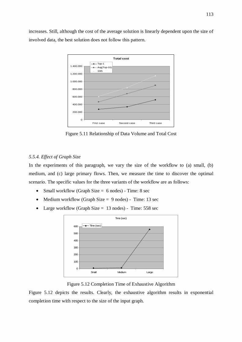
113

increases. Still, although the cost of the average solution is linearly dependent upon the size of

involved data, the best solution does not follow this pattern.

Total cost

0

200.000

400.000

600.000

800.000

1.000.000

1.200.000

1.400.000

First case Second case Third case

Top-1

Avg(Top-10)

10th

Figure 5.11 Relationship of Data Volume and Total Cost

5.5.4. Effect of Graph Size

In the experiments of this paragraph, we vary the size of the workflow to (a) small, (b)

medium, and (c) large primary flows. Then, we measure the time to discover the optimal

scenario. The specific values for the three variants of the workflow are as follows:

• Small workflow (Graph Size = 6 nodes) - Time: 8 sec

• Medium workflow (Graph Size = 9 nodes) - Time: 13 sec

• Large workflow (Graph Size = 13 nodes) - Time: 558 sec

Time (sec)

0

100

200

300

400

500

600

Small Medium Large

Time (sec)

Figure 5.12 Completion Time of Exhaustive Algorithm

Figure 5.12 depicts the results. Clearly, the exhaustive algorithm results in exponential

completion time with respect to the size of the input graph.

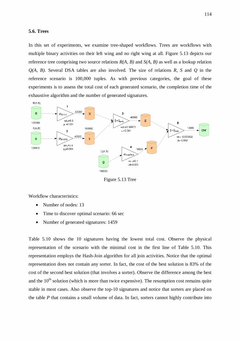
114

5.6. Trees

In this set of experiments, we examine tree-shaped workflows. Trees are workflows with

multiple binary activities on their left wing and no right wing at all. Figure 5.13 depicts our

reference tree comprising two source relations R(A, B) and S(A, B) as well as a lookup relation

Q(A, B). Several DSA tables are also involved. The size of relations R, S and Q in the

reference scenario is 100,000 tuples. As with previous categories, the goal of these

experiments is to assess the total cost of each generated scenario, the completion time of the

exhaustive algorithm and the number of generated signatures.

Figure 5.13 Tree

Workflow characteristics:

• Number of nodes: 13

• Time to discover optimal scenario: 66 sec

• Number of generated signatures: 1459

Table 5.10 shows the 10 signatures having the lowest total cost. Observe the physical

representation of the scenario with the minimal cost in the first line of Table 5.10. This

representation employs the Hash-Join algorithm for all join activities. Notice that the optimal

representation does not contain any sorter. In fact, the cost of the best solution is 83% of the

cost of the second best solution (that involves a sorter). Observe the difference among the best

and the 10th solution (which is more than twice expensive). The resumption cost remains quite

stable in most cases. Also observe the top-10 signatures and notice that sorters are placed on

the table P that contains a small volume of data. In fact, sorters cannot highly contribute into

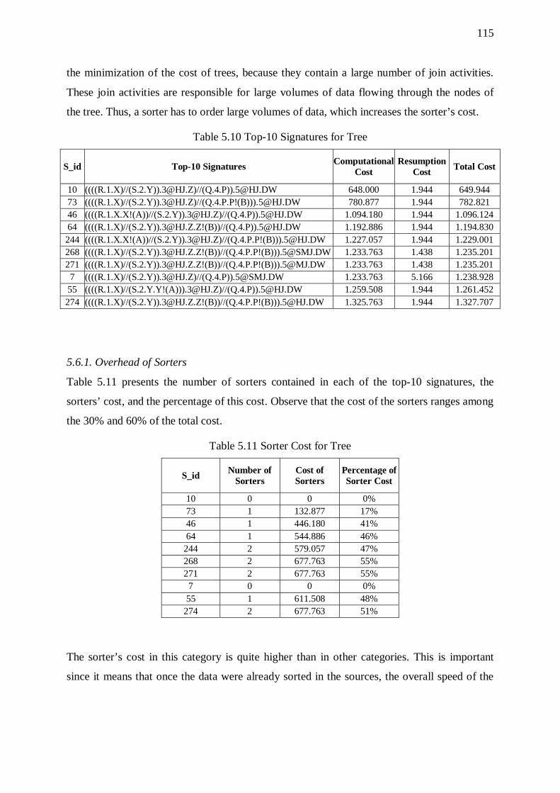
115

the minimization of the cost of trees, because they contain a large number of join activities.

These join activities are responsible for large volumes of data flowing through the nodes of

the tree. Thus, a sorter has to order large volumes of data, which increases the sorter’s cost.

Table 5.10 Top-10 Signatures for Tree

S_id Top-10 Signatures Computational Cost

Resumption Cost Total Cost

10 ((((R.1.X)//(S.2.Y)).3@HJ.Z)//(Q.4.P)).5@HJ.DW 648.000 1.944 649.944 73 ((((R.1.X)//(S.2.Y)).3@HJ.Z)//(Q.4.P.P!(B))).5@HJ.DW 780.877 1.944 782.821 46 ((((R.1.X.X!(A))//(S.2.Y)).3@HJ.Z)//(Q.4.P)).5@HJ.DW 1.094.180 1.944 1.096.124 64 ((((R.1.X)//(S.2.Y)).3@HJ.Z.Z!(B))//(Q.4.P)).5@HJ.DW 1.192.886 1.944 1.194.830 244 ((((R.1.X.X!(A))//(S.2.Y)).3@HJ.Z)//(Q.4.P.P!(B))).5@HJ.DW 1.227.057 1.944 1.229.001 268 ((((R.1.X)//(S.2.Y)).3@HJ.Z.Z!(B))//(Q.4.P.P!(B))).5@SMJ.DW 1.233.763 1.438 1.235.201 271 ((((R.1.X)//(S.2.Y)).3@HJ.Z.Z!(B))//(Q.4.P.P!(B))).5@MJ.DW 1.233.763 1.438 1.235.201

7 ((((R.1.X)//(S.2.Y)).3@HJ.Z)//(Q.4.P)).5@SMJ.DW 1.233.763 5.166 1.238.928 55 ((((R.1.X)//(S.2.Y.Y!(A))).3@HJ.Z)//(Q.4.P)).5@HJ.DW 1.259.508 1.944 1.261.452 274 ((((R.1.X)//(S.2.Y)).3@HJ.Z.Z!(B))//(Q.4.P.P!(B))).5@HJ.DW 1.325.763 1.944 1.327.707

5.6.1. Overhead of Sorters

Table 5.11 presents the number of sorters contained in each of the top-10 signatures, the

sorters’ cost, and the percentage of this cost. Observe that the cost of the sorters ranges among

the 30% and 60% of the total cost.

Table 5.11 Sorter Cost for Tree

S_id Number of Sorters

Cost of Sorters

Percentage of Sorter Cost

10 0 0 0% 73 1 132.877 17% 46 1 446.180 41% 64 1 544.886 46%

244 2 579.057 47% 268 2 677.763 55% 271 2 677.763 55% 7 0 0 0% 55 1 611.508 48%

274 2 677.763 51%

The sorter’s cost in this category is quite higher than in other categories. This is important

since it means that once the data were already sorted in the sources, the overall speed of the

116

scenario could be significantly enhanced. Still, as already mentioned, the intermediate sorters

incur high costs due to the high volume of sorted data.

5.6.2. Effect of Input Size

In the reference scenario, each of the sources R, S and Q contains 100,000 rows. We have also

experimented by varying the size of data extracted from each source to 200,000 rows. The

second experiment returns the same 6 solutions out of the top-10 list of the reference scenario.

We have also observed that the total cost of the optimal solution in all cases is practically

linearly dependent upon the input size. This observation holds also for the average cost of the

top-10 signatures and the 10th solution.

5.6.3. Effect of the Overall Selectivity of the Workflow

In the experiments of this paragraph, we modify the selectivities of the activities of the tree in

such a way, that small, medium or large volumes of data reach the output. In particular, we

appropriately tune the selectivities of all the activities of the workflow, so that the ratio of data

of the final, target relation over the input data is 0.1, 0.3, 0.5, 0.7. Table 5.12 shows the size of

the output after each activity of the workflow (activity numbers in the first line of the table

refer to the numbers of Figure 5.13).

Table 5.12 Size of the Output of each Activity of the Scenario in Fig. 5.13

1 2 3 4 5 Case of 0.1 0.3|R| 0.4|R| 0.4|R| 0.1|R| 0.1|R| Case of 0.3 0.6|R| 0.8|R| 0.8|R| 0.3|R| 0.3|R|

Case of 0.5 0.7|R| 0.8|R| 0.8|R| 0.5|R| 0.5|R| Case of 0.7 0.9|R| 0.9|R| 0.9|R| 0.9|R| 0.7|R|

Table 5.13 depicts the effect of data volume propagated towards the warehouse. Observe that

the optimal solution remains the same, irrespectively of the data volumes that are propagated

to the warehouse. A lesson learned here is the stability of the best solution, which, at the same

time, does not include any sorters. As the volume of data is increased, one third of the top-10

solutions are different. The costs in the different scenarios increase mainly depending upon

the join selectivities: as the amount of data produced by the joins increases, the overall cost

follows this increase. For example, the reason for the significant cost increase between 0.1|R|

and 0.3|R| is due to the drastic increase of the selectivity of the join activity 3, which rises

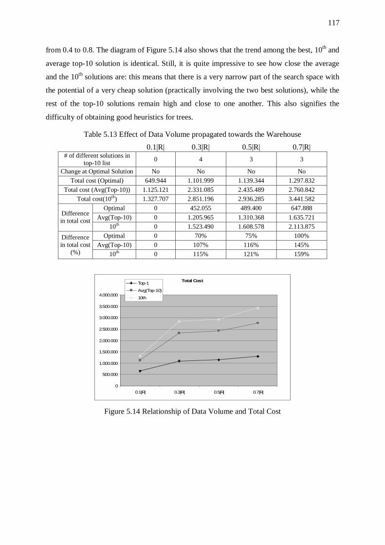
117

from 0.4 to 0.8. The diagram of Figure 5.14 also shows that the trend among the best, 10th and

average top-10 solution is identical. Still, it is quite impressive to see how close the average

and the 10th solutions are: this means that there is a very narrow part of the search space with

the potential of a very cheap solution (practically involving the two best solutions), while the

rest of the top-10 solutions remain high and close to one another. This also signifies the

difficulty of obtaining good heuristics for trees.

Table 5.13 Effect of Data Volume propagated towards the Warehouse

0.1|R| 0.3|R| 0.5|R| 0.7|R| # of different solutions in

top-10 list 0 4 3 3

Change at Optimal Solution No No No No

Total cost (Optimal) 649.944 1.101.999 1.139.344 1.297.832

Total cost (Avg(Top-10)) 1.125.121 2.331.085 2.435.489 2.760.842

Total cost(10th) 1.327.707 2.851.196 2.936.285 3.441.582

Optimal 0 452.055 489.400 647.888

Avg(Top-10) 0 1.205.965 1.310.368 1.635.721 Difference in total cost

10th 0 1.523.490 1.608.578 2.113.875

Optimal 0 70% 75% 100%

Avg(Top-10) 0 107% 116% 145% Difference in total cost

(%) 10th 0 115% 121% 159%

Total Cost

0

500.000

1.000.000

1.500.000

2.000.000

2.500.000

3.000.000

3.500.000

4.000.000

0.1|R| 0.3|R| 0.5|R| 0.7|R|

Top-1

Avg(Top-10)

10th

Figure 5.14 Relationship of Data Volume and Total Cost

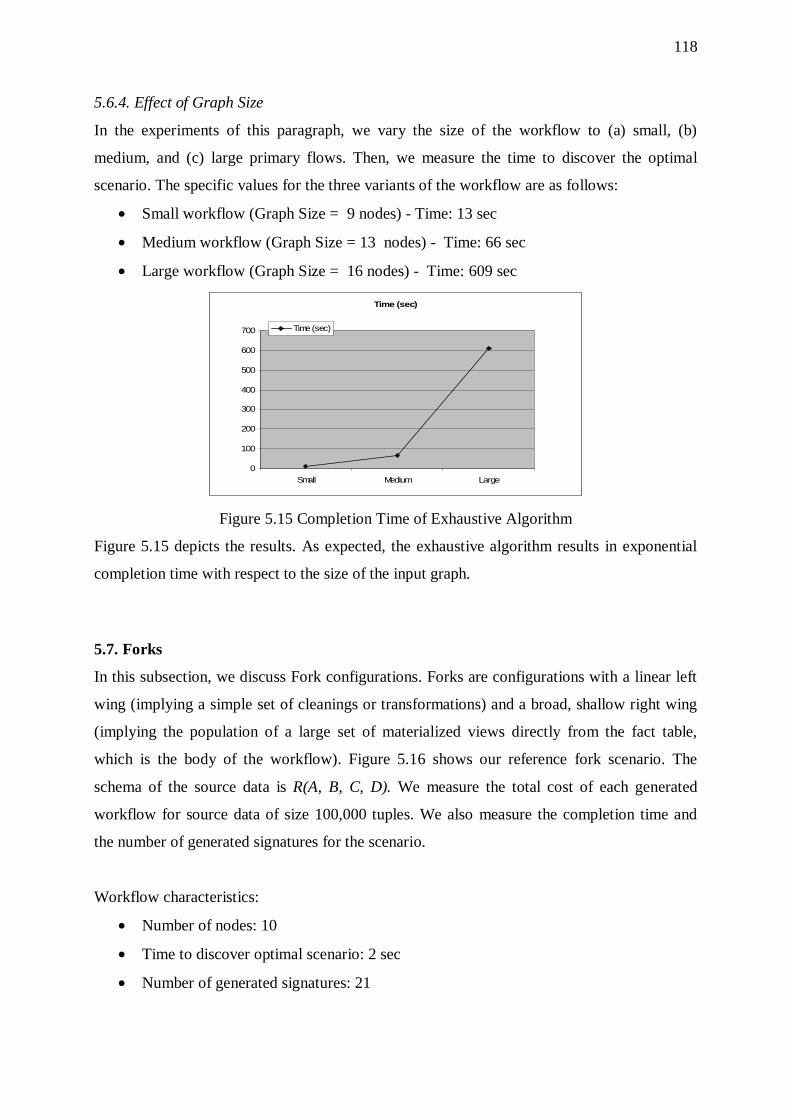
118

5.6.4. Effect of Graph Size

In the experiments of this paragraph, we vary the size of the workflow to (a) small, (b)

medium, and (c) large primary flows. Then, we measure the time to discover the optimal

scenario. The specific values for the three variants of the workflow are as follows:

• Small workflow (Graph Size = 9 nodes) - Time: 13 sec

• Medium workflow (Graph Size = 13 nodes) - Time: 66 sec

• Large workflow (Graph Size = 16 nodes) - Time: 609 sec

Time (sec)

0

100

200

300

400

500

600

700

Small Medium Large

Time (sec)

Figure 5.15 Completion Time of Exhaustive Algorithm

Figure 5.15 depicts the results. As expected, the exhaustive algorithm results in exponential

completion time with respect to the size of the input graph.

5.7. Forks

In this subsection, we discuss Fork configurations. Forks are configurations with a linear left

wing (implying a simple set of cleanings or transformations) and a broad, shallow right wing

(implying the population of a large set of materialized views directly from the fact table,

which is the body of the workflow). Figure 5.16 shows our reference fork scenario. The

schema of the source data is R(A, B, C, D). We measure the total cost of each generated

workflow for source data of size 100,000 tuples. We also measure the completion time and

the number of generated signatures for the scenario.

Workflow characteristics:

• Number of nodes: 10

• Time to discover optimal scenario: 2 sec

• Number of generated signatures: 21

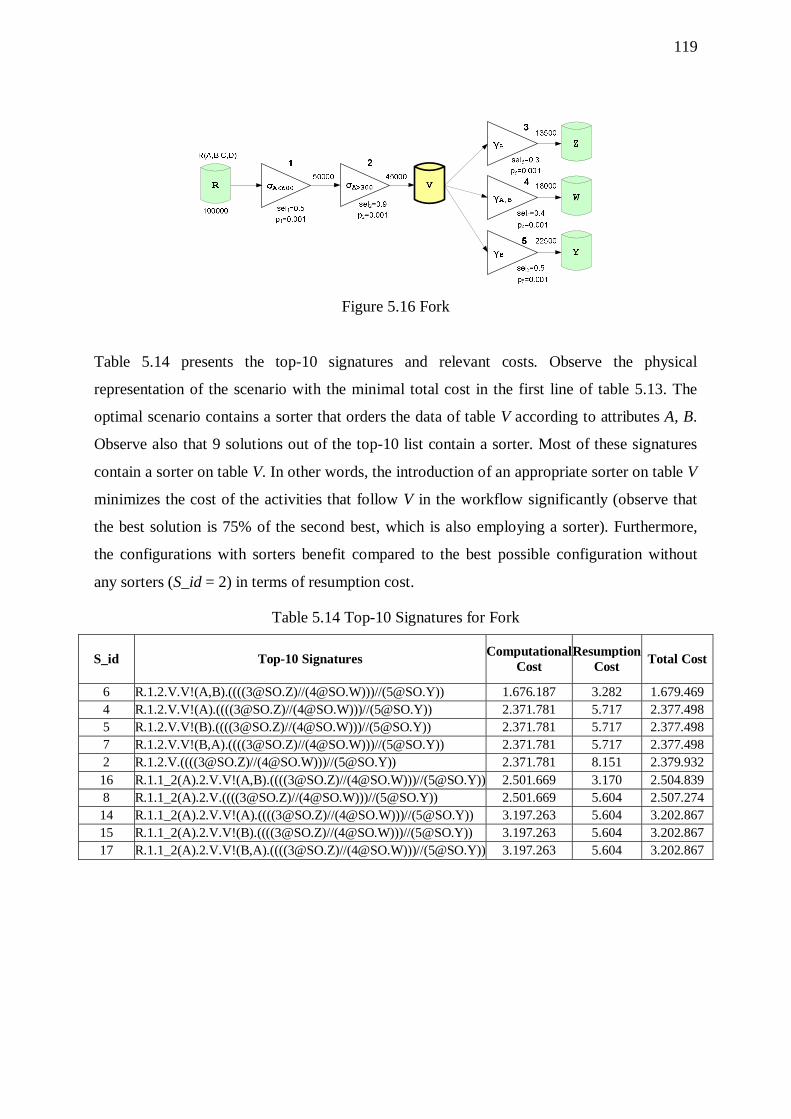
119

Figure 5.16 Fork

Table 5.14 presents the top-10 signatures and relevant costs. Observe the physical

representation of the scenario with the minimal total cost in the first line of table 5.13. The

optimal scenario contains a sorter that orders the data of table V according to attributes A, B.

Observe also that 9 solutions out of the top-10 list contain a sorter. Most of these signatures

contain a sorter on table V. In other words, the introduction of an appropriate sorter on table V

minimizes the cost of the activities that follow V in the workflow significantly (observe that

the best solution is 75% of the second best, which is also employing a sorter). Furthermore,

the configurations with sorters benefit compared to the best possible configuration without

any sorters (S_id = 2) in terms of resumption cost.

Table 5.14 Top-10 Signatures for Fork

S_id Top-10 Signatures Computational Cost

Resumption Cost Total Cost

6 R.1.2.V.V!(A,B).((((3@SO.Z)//(4@SO.W)))//(5@SO.Y)) 1.676.187 3.282 1.679.469 4 R.1.2.V.V!(A).((((3@SO.Z)//(4@SO.W)))//(5@SO.Y)) 2.371.781 5.717 2.377.498 5 R.1.2.V.V!(B).((((3@SO.Z)//(4@SO.W)))//(5@SO.Y)) 2.371.781 5.717 2.377.498 7 R.1.2.V.V!(B,A).((((3@SO.Z)//(4@SO.W)))//(5@SO.Y)) 2.371.781 5.717 2.377.498 2 R.1.2.V.((((3@SO.Z)//(4@SO.W)))//(5@SO.Y)) 2.371.781 8.151 2.379.932 16 R.1.1_2(A).2.V.V!(A,B).((((3@SO.Z)//(4@SO.W)))//(5@SO.Y)) 2.501.669 3.170 2.504.839 8 R.1.1_2(A).2.V.((((3@SO.Z)//(4@SO.W)))//(5@SO.Y)) 2.501.669 5.604 2.507.274 14 R.1.1_2(A).2.V.V!(A).((((3@SO.Z)//(4@SO.W)))//(5@SO.Y)) 3.197.263 5.604 3.202.867 15 R.1.1_2(A).2.V.V!(B).((((3@SO.Z)//(4@SO.W)))//(5@SO.Y)) 3.197.263 5.604 3.202.867 17 R.1.1_2(A).2.V.V!(B,A).((((3@SO.Z)//(4@SO.W)))//(5@SO.Y)) 3.197.263 5.604 3.202.867

120

5.7.1. Overhead of Sorters

Table 5.15 presents the number of sorters contained in each of the top-10 signatures, the

sorters’ cost, and the percentage of this cost. Observe that the cost of the sorters ranges among

the 30% and 60% of the total cost.

Table 5.15 Sorter Cost for Fork

S_id Number of Sorters

Cost of Sorters

Percentage of Sorter Cost

6 1 695.594 41% 4 1 695.594 29% 5 1 695.594 29% 7 1 695.594 29% 2 0 0 0% 16 2 1.526.076 61% 8 1 830.482 33% 14 2 1.526.076 48% 15 2 1.526.076 48% 17 2 1.526.076 48%

5.7.2. Effect of Input Size

In the reference scenario, the source R contains 100,000 rows. We have also experimented by

varying the size of data extracted from source R to 150,000 and 200,000 rows. These

experiments return the same top-10 solutions with the reference scenario. We have also

observed that the total cost of the optimal solution in all cases is practically linearly dependent

upon the input size. This observation holds also for the average cost of the top-10 signatures

and the 10th solution.

5.7.3. Effect of the Overall Selectivity of the Workflow

In the experiments of this paragraph, we modify the selectivity values of the workflow in such

a way, that small, medium or large volumes of data reach the output. In particular, we

appropriately tune the selectivities, so that the ratio of the output data over the input data is:

0.1, 0.3, 0.5 or 0.7. In other words, we try to assess the impact of the overall selectivity of the

workflow to the overall cost.

Table 5.16 shows the size of the output after each activity (activity numbers in the first line of

the table refer to the numbers of Figure 5.16.

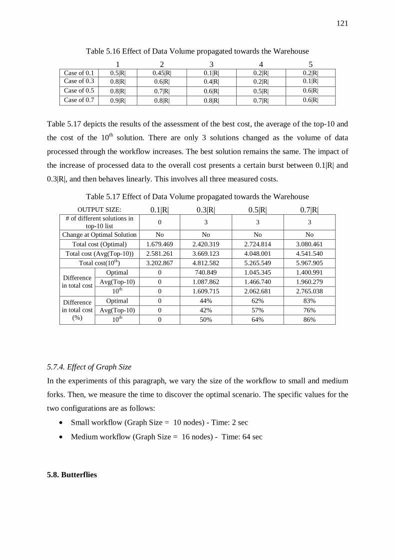
121

Table 5.16 Effect of Data Volume propagated towards the Warehouse

1 2 3 4 5 Case of 0.1 0.5|R| 0.45|R| 0.1|R| 0.2|R| 0.2|R| Case of 0.3 0.8|R| 0.6|R| 0.4|R| 0.2|R| 0.1|R|

Case of 0.5 0.8|R| 0.7|R| 0.6|R| 0.5|R| 0.6|R|

Case of 0.7 0.9|R| 0.8|R| 0.8|R| 0.7|R| 0.6|R|

Table 5.17 depicts the results of the assessment of the best cost, the average of the top-10 and

the cost of the 10th solution. There are only 3 solutions changed as the volume of data

processed through the workflow increases. The best solution remains the same. The impact of

the increase of processed data to the overall cost presents a certain burst between 0.1|R| and

0.3|R|, and then behaves linearly. This involves all three measured costs.

Table 5.17 Effect of Data Volume propagated towards the Warehouse

OUTPUT SIZE: 0.1|R| 0.3|R| 0.5|R| 0.7|R| # of different solutions in

top-10 list 0 3 3 3

Change at Optimal Solution No No No No

Total cost (Optimal) 1.679.469 2.420.319 2.724.814 3.080.461

Total cost (Avg(Top-10)) 2.581.261 3.669.123 4.048.001 4.541.540

Total cost(10th) 3.202.867 4.812.582 5.265.549 5.967.905

Optimal 0 740.849 1.045.345 1.400.991

Avg(Top-10) 0 1.087.862 1.466.740 1.960.279 Difference in total cost

10th 0 1.609.715 2.062.681 2.765.038

Optimal 0 44% 62% 83%

Avg(Top-10) 0 42% 57% 76% Difference in total cost

(%) 10th 0 50% 64% 86%

5.7.4. Effect of Graph Size

In the experiments of this paragraph, we vary the size of the workflow to small and medium

forks. Then, we measure the time to discover the optimal scenario. The specific values for the

two configurations are as follows:

• Small workflow (Graph Size = 10 nodes) - Time: 2 sec

• Medium workflow (Graph Size = 16 nodes) - Time: 64 sec

5.8. Butterflies

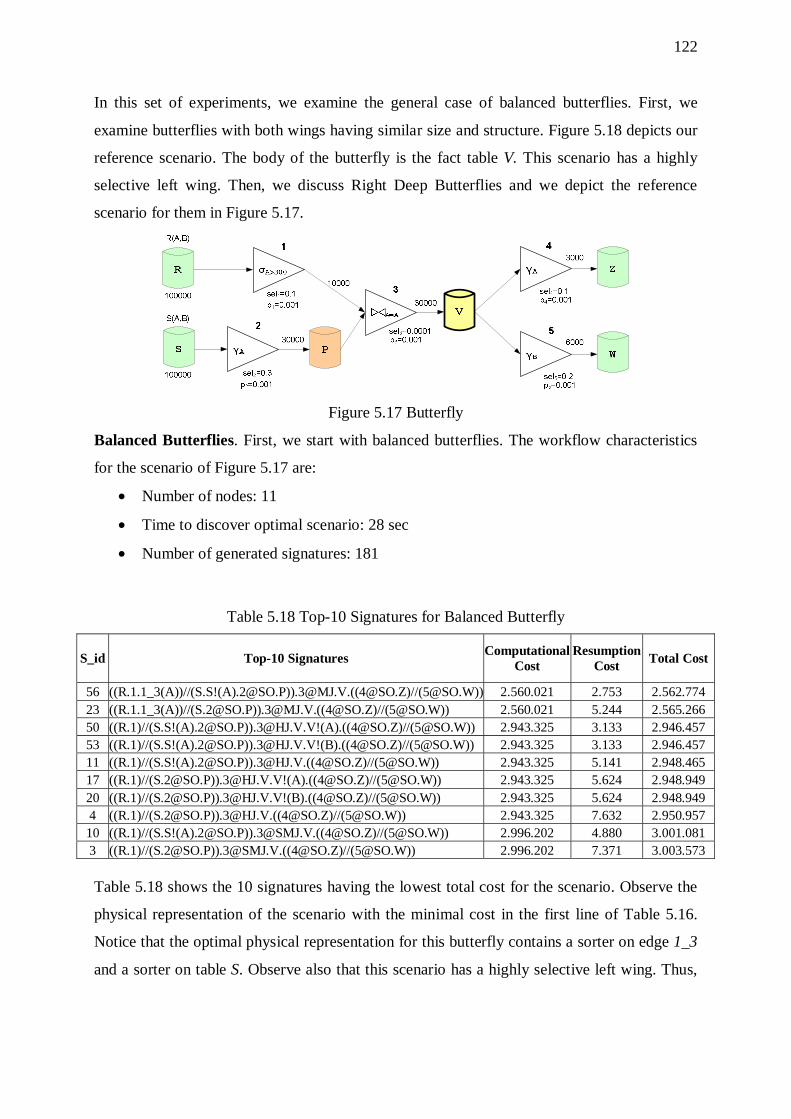
122

In this set of experiments, we examine the general case of balanced butterflies. First, we

examine butterflies with both wings having similar size and structure. Figure 5.18 depicts our

reference scenario. The body of the butterfly is the fact table V. This scenario has a highly

selective left wing. Then, we discuss Right Deep Butterflies and we depict the reference

scenario for them in Figure 5.17.

Figure 5.17 Butterfly

Balanced Butterflies. First, we start with balanced butterflies. The workflow characteristics

for the scenario of Figure 5.17 are:

• Number of nodes: 11

• Time to discover optimal scenario: 28 sec

• Number of generated signatures: 181

Table 5.18 Top-10 Signatures for Balanced Butterfly

S_id Top-10 Signatures Computational Cost

Resumption Cost Total Cost

56 ((R.1.1_3(A))//(S.S!(A).2@SO.P)).3@MJ.V.((4@SO.Z)//(5@SO.W)) 2.560.021 2.753 2.562.774 23 ((R.1.1_3(A))//(S.2@SO.P)).3@MJ.V.((4@SO.Z)//(5@SO.W)) 2.560.021 5.244 2.565.266 50 ((R.1)//(S.S!(A).2@SO.P)).3@HJ.V.V!(A).((4@SO.Z)//(5@SO.W)) 2.943.325 3.133 2.946.457 53 ((R.1)//(S.S!(A).2@SO.P)).3@HJ.V.V!(B).((4@SO.Z)//(5@SO.W)) 2.943.325 3.133 2.946.457 11 ((R.1)//(S.S!(A).2@SO.P)).3@HJ.V.((4@SO.Z)//(5@SO.W)) 2.943.325 5.141 2.948.465 17 ((R.1)//(S.2@SO.P)).3@HJ.V.V!(A).((4@SO.Z)//(5@SO.W)) 2.943.325 5.624 2.948.949 20 ((R.1)//(S.2@SO.P)).3@HJ.V.V!(B).((4@SO.Z)//(5@SO.W)) 2.943.325 5.624 2.948.949 4 ((R.1)//(S.2@SO.P)).3@HJ.V.((4@SO.Z)//(5@SO.W)) 2.943.325 7.632 2.950.957 10 ((R.1)//(S.S!(A).2@SO.P)).3@SMJ.V.((4@SO.Z)//(5@SO.W)) 2.996.202 4.880 3.001.081 3 ((R.1)//(S.2@SO.P)).3@SMJ.V.((4@SO.Z)//(5@SO.W)) 2.996.202 7.371 3.003.573 Table 5.18 shows the 10 signatures having the lowest total cost for the scenario. Observe the

physical representation of the scenario with the minimal cost in the first line of Table 5.16.

Notice that the optimal physical representation for this butterfly contains a sorter on edge 1_3

and a sorter on table S. Observe also that this scenario has a highly selective left wing. Thus,

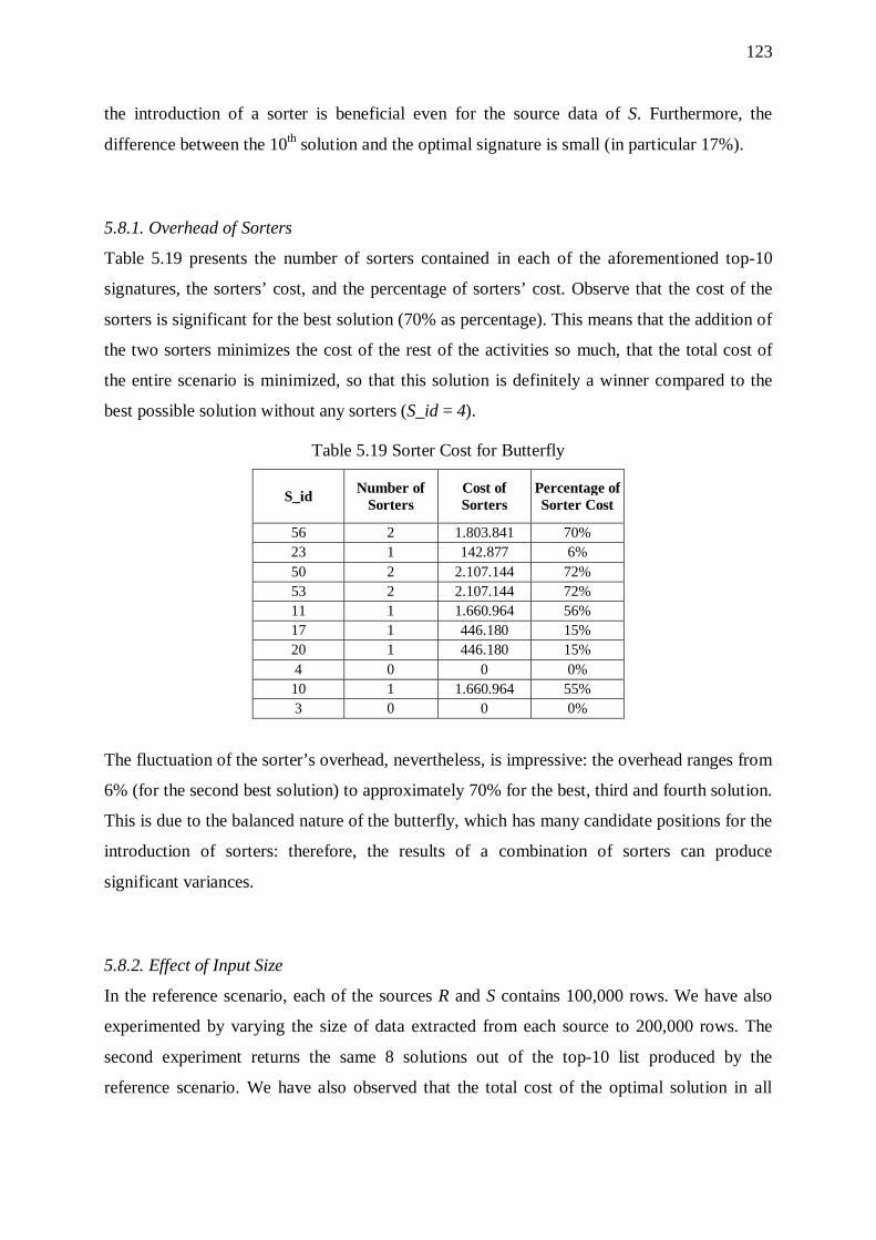
123

the introduction of a sorter is beneficial even for the source data of S. Furthermore, the

difference between the 10th solution and the optimal signature is small (in particular 17%).

5.8.1. Overhead of Sorters

Table 5.19 presents the number of sorters contained in each of the aforementioned top-10

signatures, the sorters’ cost, and the percentage of sorters’ cost. Observe that the cost of the

sorters is significant for the best solution (70% as percentage). This means that the addition of

the two sorters minimizes the cost of the rest of the activities so much, that the total cost of

the entire scenario is minimized, so that this solution is definitely a winner compared to the

best possible solution without any sorters (S_id = 4).

Table 5.19 Sorter Cost for Butterfly

S_id Number of Sorters

Cost of Sorters

Percentage of Sorter Cost

56 2 1.803.841 70% 23 1 142.877 6% 50 2 2.107.144 72% 53 2 2.107.144 72% 11 1 1.660.964 56% 17 1 446.180 15% 20 1 446.180 15% 4 0 0 0% 10 1 1.660.964 55% 3 0 0 0%

The fluctuation of the sorter’s overhead, nevertheless, is impressive: the overhead ranges from

6% (for the second best solution) to approximately 70% for the best, third and fourth solution.

This is due to the balanced nature of the butterfly, which has many candidate positions for the

introduction of sorters: therefore, the results of a combination of sorters can produce

significant variances.

5.8.2. Effect of Input Size

In the reference scenario, each of the sources R and S contains 100,000 rows. We have also

experimented by varying the size of data extracted from each source to 200,000 rows. The

second experiment returns the same 8 solutions out of the top-10 list produced by the

reference scenario. We have also observed that the total cost of the optimal solution in all

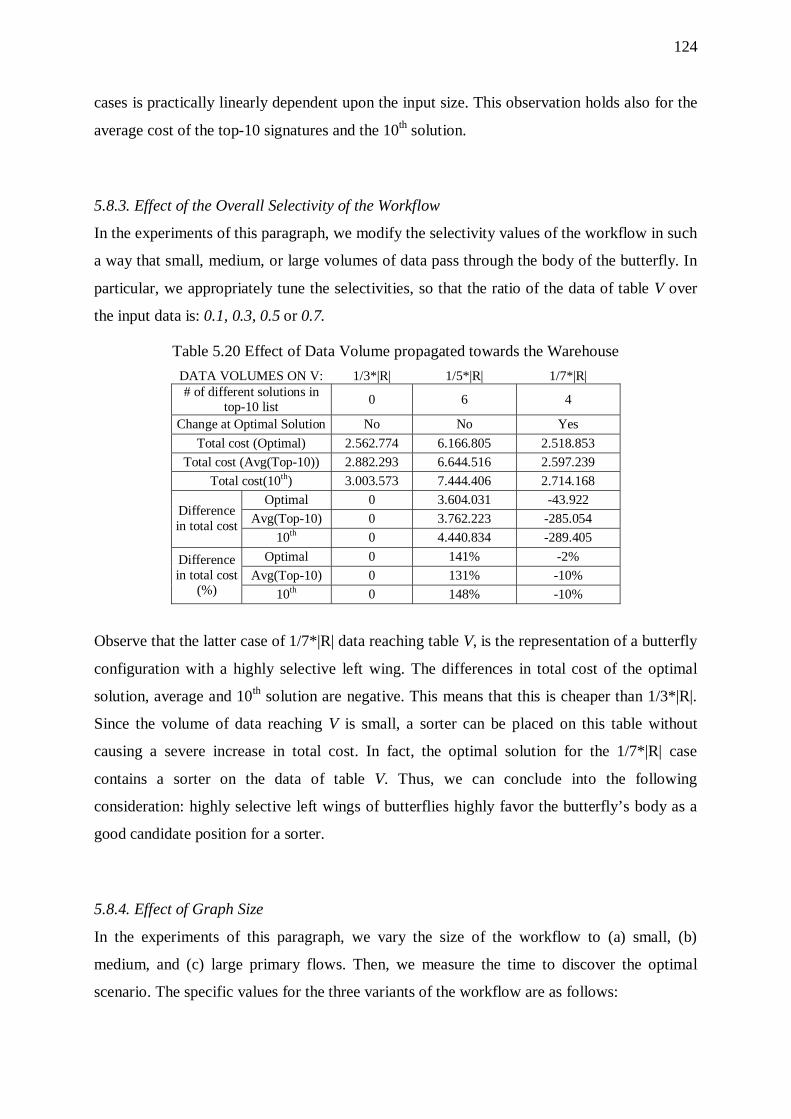
124

cases is practically linearly dependent upon the input size. This observation holds also for the

average cost of the top-10 signatures and the 10th solution.

5.8.3. Effect of the Overall Selectivity of the Workflow

In the experiments of this paragraph, we modify the selectivity values of the workflow in such

a way that small, medium, or large volumes of data pass through the body of the butterfly. In

particular, we appropriately tune the selectivities, so that the ratio of the data of table V over

the input data is: 0.1, 0.3, 0.5 or 0.7.

Table 5.20 Effect of Data Volume propagated towards the Warehouse

DATA VOLUMES ON V: 1/3*|R| 1/5*|R| 1/7*|R| # of different solutions in

top-10 list 0 6 4

Change at Optimal Solution No No Yes

Total cost (Optimal) 2.562.774 6.166.805 2.518.853

Total cost (Avg(Top-10)) 2.882.293 6.644.516 2.597.239

Total cost(10th) 3.003.573 7.444.406 2.714.168

Optimal 0 3.604.031 -43.922

Avg(Top-10) 0 3.762.223 -285.054 Difference in total cost

10th 0 4.440.834 -289.405

Optimal 0 141% -2%

Avg(Top-10) 0 131% -10% Difference in total cost

(%) 10th 0 148% -10%

Observe that the latter case of 1/7*|R| data reaching table V, is the representation of a butterfly

configuration with a highly selective left wing. The differences in total cost of the optimal

solution, average and 10th solution are negative. This means that this is cheaper than 1/3*|R|.

Since the volume of data reaching V is small, a sorter can be placed on this table without

causing a severe increase in total cost. In fact, the optimal solution for the 1/7*|R| case

contains a sorter on the data of table V. Thus, we can conclude into the following

consideration: highly selective left wings of butterflies highly favor the butterfly’s body as a

good candidate position for a sorter.

5.8.4. Effect of Graph Size

In the experiments of this paragraph, we vary the size of the workflow to (a) small, (b)

medium, and (c) large primary flows. Then, we measure the time to discover the optimal

scenario. The specific values for the three variants of the workflow are as follows:

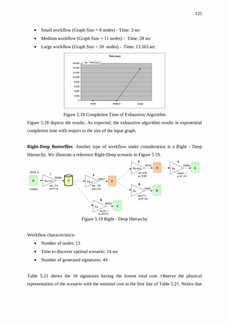
125

• Small workflow (Graph Size = 8 nodes) - Time: 3 sec

• Medium workflow (Graph Size = 11 nodes) - Time: 28 sec

• Large workflow (Graph Size = 20 nodes) - Time: 13.563 sec

Time (sec)

0

2.000

4.000

6.000

8.000

10.000

12.000

14.000

16.000

Small Medium Large

Time (sec)

Figure 5.18 Completion Time of Exhaustive Algorithm

Figure 5.18 depicts the results. As expected, the exhaustive algorithm results in exponential

completion time with respect to the size of the input graph.

Right-Deep Butterflies. Another type of workflow under consideration is a Right - Deep

Hierarchy. We illustrate a reference Right-Deep scenario in Figure 5.19.

Figure 5.19 Right - Deep Hierarchy

Workflow characteristics:

• Number of nodes: 13

• Time to discover optimal scenario: 14 sec

• Number of generated signatures: 49

Table 5.21 shows the 10 signatures having the lowest total cost. Observe the physical

representation of the scenario with the minimal cost in the first line of Table 5.21. Notice that

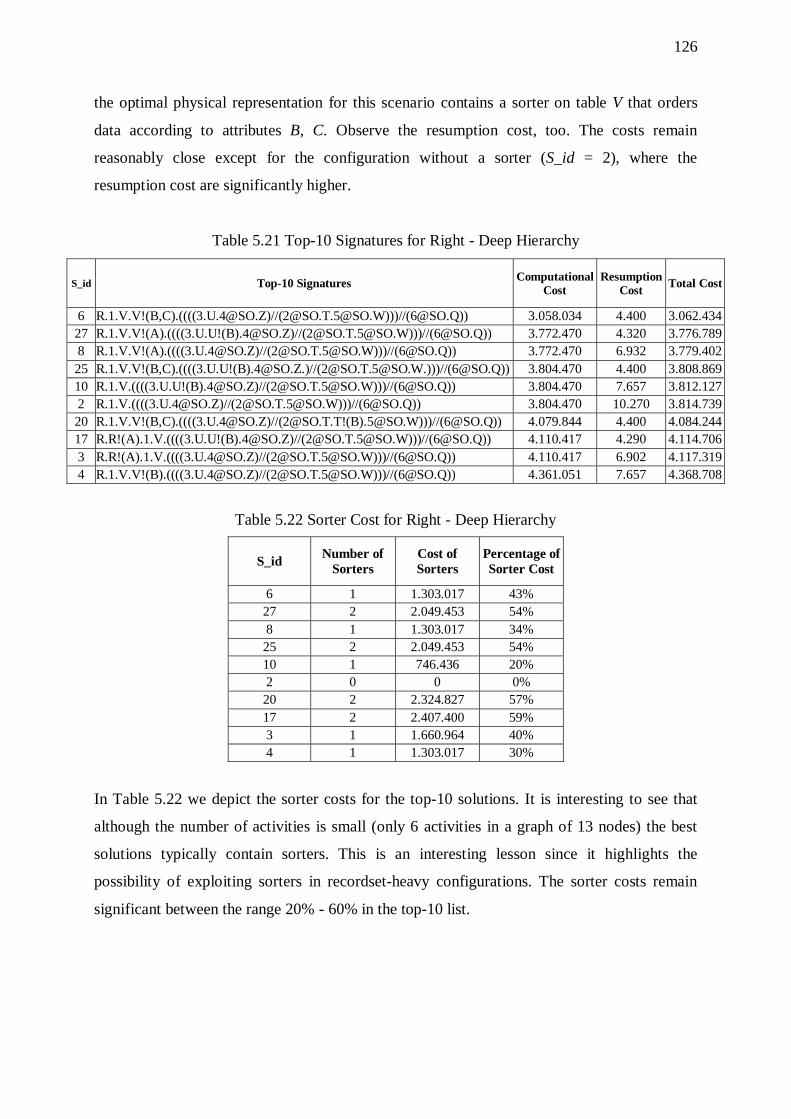
126

the optimal physical representation for this scenario contains a sorter on table V that orders

data according to attributes B, C. Observe the resumption cost, too. The costs remain

reasonably close except for the configuration without a sorter (S_id = 2), where the

resumption cost are significantly higher.

Table 5.21 Top-10 Signatures for Right - Deep Hierarchy

S_id Top-10 Signatures Computational Cost

Resumption Cost

Total Cost

6 R.1.V.V!(B,C).((((3.U.4@SO.Z)//(2@SO.T.5@SO.W)))//(6@SO.Q)) 3.058.034 4.400 3.062.434 27 R.1.V.V!(A).((((3.U.U!(B).4@SO.Z)//(2@SO.T.5@SO.W)))//(6@SO.Q)) 3.772.470 4.320 3.776.789 8 R.1.V.V!(A).((((3.U.4@SO.Z)//(2@SO.T.5@SO.W)))//(6@SO.Q)) 3.772.470 6.932 3.779.402 25 R.1.V.V!(B,C).((((3.U.U!(B).4@SO.Z.)//(2@SO.T.5@SO.W.)))//(6@SO.Q)) 3.804.470 4.400 3.808.869 10 R.1.V.((((3.U.U!(B).4@SO.Z)//(2@SO.T.5@SO.W)))//(6@SO.Q)) 3.804.470 7.657 3.812.127 2 R.1.V.((((3.U.4@SO.Z)//(2@SO.T.5@SO.W)))//(6@SO.Q)) 3.804.470 10.270 3.814.739 20 R.1.V.V!(B,C).((((3.U.4@SO.Z)//(2@SO.T.T!(B).5@SO.W)))//(6@SO.Q)) 4.079.844 4.400 4.084.244 17 R.R!(A).1.V.((((3.U.U!(B).4@SO.Z)//(2@SO.T.5@SO.W)))//(6@SO.Q)) 4.110.417 4.290 4.114.706 3 R.R!(A).1.V.((((3.U.4@SO.Z)//(2@SO.T.5@SO.W)))//(6@SO.Q)) 4.110.417 6.902 4.117.319 4 R.1.V.V!(B).((((3.U.4@SO.Z)//(2@SO.T.5@SO.W)))//(6@SO.Q)) 4.361.051 7.657 4.368.708

Table 5.22 Sorter Cost for Right - Deep Hierarchy

S_id Number of Sorters

Cost of Sorters

Percentage of Sorter Cost

6 1 1.303.017 43% 27 2 2.049.453 54% 8 1 1.303.017 34% 25 2 2.049.453 54% 10 1 746.436 20% 2 0 0 0% 20 2 2.324.827 57% 17 2 2.407.400 59% 3 1 1.660.964 40% 4 1 1.303.017 30%

In Table 5.22 we depict the sorter costs for the top-10 solutions. It is interesting to see that

although the number of activities is small (only 6 activities in a graph of 13 nodes) the best

solutions typically contain sorters. This is an interesting lesson since it highlights the

possibility of exploiting sorters in recordset-heavy configurations. The sorter costs remain

significant between the range 20% - 60% in the top-10 list.

127

5.8.5. Effect of Input Size

In the reference scenario, the source R contains 100,000 rows. We have also experimented by

varying the size of data extracted from source R to 150,000 and 200,000 rows. All

experiments return the same top-10 list as the reference scenario. We have also observed that

the total cost of the optimal solution in all cases is practically linearly dependent upon the

input size. This observation holds also for the average cost of the top-10 signatures and the

10th solution.

5.8.6. Effect of Graph Size

In the experiments of this paragraph, we vary the size of the workflow to (a) small, (b)

medium, and (c) large primary flows. Then, we measure the time to discover the optimal

scenario. The specific values for the three variants of the workflow are as follows:

• Small workflow (Graph Size = 11 nodes) - Time: 5 sec

• Medium workflow (Graph Size = 13 nodes) - Time: 14 sec

• Large workflow (Graph Size = 20 nodes) - Time: 311 sec

Clearly, the exhaustive algorithm results in exponential completion time with respect to the

size of the input graph.

5.8.7. Effect of Complexity (Depth and Fan-out) of the Right Wing

In this set of experiments, we vary the following metrics: the size, the depth and the average

fan-out (we count the average fan-out of the recordsets contained in the right wing) of the

right wing of the butterfly. Then, we measure the candidate positions for sorters and the

completion time of the exhaustive algorithm. Table 5.23 depicts the results.

Table 5.23 Effect of Depth and Fan-out

First case Second case Third case Fourth case

# of nodes on the right wing 8 10 14 15

Depth 4 6 4 6

Avg(Fan-out) 2 0.8 2.3 2

Candidate positions for sorters 2 3 3 6

Completion Time (sec) 5 14 59 311

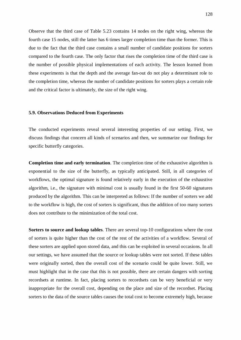
128

Observe that the third case of Table 5.23 contains 14 nodes on the right wing, whereas the

fourth case 15 nodes, still the latter has 6 times larger completion time than the former. This is

due to the fact that the third case contains a small number of candidate positions for sorters

compared to the fourth case. The only factor that rises the completion time of the third case is

the number of possible physical implementations of each activity. The lesson learned from

these experiments is that the depth and the average fan-out do not play a determinant role to

the completion time, whereas the number of candidate positions for sorters plays a certain role

and the critical factor is ultimately, the size of the right wing.

5.9. Observations Deduced from Experiments

The conducted experiments reveal several interesting properties of our setting. First, we

discuss findings that concern all kinds of scenarios and then, we summarize our findings for

specific butterfly categories.

Completion time and early termination. The completion time of the exhaustive algorithm is

exponential to the size of the butterfly, as typically anticipated. Still, in all categories of

workflows, the optimal signature is found relatively early in the execution of the exhaustive

algorithm, i.e., the signature with minimal cost is usually found in the first 50-60 signatures

produced by the algorithm. This can be interpreted as follows: If the number of sorters we add

to the workflow is high, the cost of sorters is significant, thus the addition of too many sorters

does not contribute to the minimization of the total cost.

Sorters to source and lookup tables. There are several top-10 configurations where the cost

of sorters is quite higher than the cost of the rest of the activities of a workflow. Several of

these sorters are applied upon stored data, and this can be exploited in several occasions. In all

our settings, we have assumed that the source or lookup tables were not sorted. If these tables

were originally sorted, then the overall cost of the scenario could be quite lower. Still, we

must highlight that in the case that this is not possible, there are certain dangers with sorting

recordsets at runtime. In fact, placing sorters to recordsets can be very beneficial or very

inappropriate for the overall cost, depending on the place and size of the recordset. Placing

sorters to the data of the source tables causes the total cost to become extremely high, because

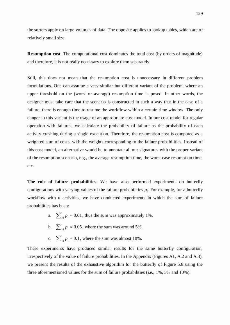
129

the sorters apply on large volumes of data. The opposite applies to lookup tables, which are of

relatively small size.

Resumption cost. The computational cost dominates the total cost (by orders of magnitude)

and therefore, it is not really necessary to explore them separately.

Still, this does not mean that the resumption cost is unnecessary in different problem

formulations. One can assume a very similar but different variant of the problem, where an

upper threshold on the (worst or average) resumption time is posed. In other words, the

designer must take care that the scenario is constructed in such a way that in the case of a

failure, there is enough time to resume the workflow within a certain time window. The only

danger in this variant is the usage of an appropriate cost model. In our cost model for regular

operation with failures, we calculate the probability of failure as the probability of each

activity crashing during a single execution. Therefore, the resumption cost is computed as a

weighted sum of costs, with the weights corresponding to the failure probabilities. Instead of

this cost model, an alternative would be to annotate all our signatures with the proper variant

of the resumption scenario, e.g., the average resumption time, the worst case resumption time,

etc.

The role of failure probabilities. We have also performed experiments on butterfly

configurations with varying values of the failure probabilities pi. For example, for a butterfly

workflow with n activities, we have conducted experiments in which the sum of failure

probabilities has been:

a. 01.01

≈∑ =

n

i ip , thus the sum was approximately 1%.

b. 05.01

≈∑ =

n

i ip , where the sum was around 5%.

c. 1.01

≈∑ =

n

i ip , where the sum was almost 10%.

These experiments have produced similar results for the same butterfly configuration,

irrespectively of the value of failure probabilities. In the Appendix (Figures A1, A.2 and A.3),

we present the results of the exhaustive algorithm for the butterfly of Figure 5.8 using the

three aforementioned values for the sum of failure probabilities (i.e., 1%, 5% and 10%).

130

Now, we discuss findings that pertain to specific categories of butterflies.

Lines. We can observe that the generated space of alternative physical representations of a

Linear scenario is linear to the size of the workflow (without addition of sorters). For

example, consider two successive activities with 2 and 3 physical implementations

respectively. Then, the number of generated signatures is 2∗3=6. In our experiments we have

also observed that due to the selectivities involved, the left wing might eventually determine

the overall cost (and therefore, placing filters as early as possible is beneficial, as one would

typically expect).

Butterflies with no right wing. In principle, the butterflies that comprise just a left wing are

not particularly improved when sorters are involved. In particular, we have observed that the

introduction of sorters in Wishbones and Trees does not lead to the reduction of the total cost

of the workflow. There are certain cases, in trees, however, where sorters might help –

provided that the data pushed through the involved branch has a small size.

Forks. Sorters are highly beneficial for forks. This is clearly anticipated since a fork involves

a high reusability of the butterfly’s body. Therefore, the body of the butterfly is typically a

good candidate for a sorter.

Balanced butterflies. The most general case of butterflies is characterized by many candidate

positions for sorters. Overall, the introduction of sorters appears to benefit the overall cost.

Moreover, the sorters significantly improve the resumption cost. The body of the butterfly is a

good candidate to place a sorter, especially when the left wing is highly selective.

Butterflies with a right-deep hierarchy. These butterflies behave more or less like the

general case of balanced butterflies. The size of the right wing is the major determinant of the

overall completion cost of the exhaustive algorithm.

131

CHAPTER 6. CONCLUSIONS AND FUTURE WORK

6.1 Conclusions

6.2 Future Work

6.1. Conclusions

In this work, we have dealt with the problem of mapping a logical ETL scenario to its

alternative physical representations. Each logical ETL workflow is an abstract design that has

to be implemented physically, i.e., mapped to a combination of executable scripts/programs

that perform the actual ETL process. The activities of the workflow can be implemented using

various algorithmic methods, each with its own cost in terms of time or system resources. The

purpose of this work has been to discover the best possible physical implementation of a

given logical ETL workflow. To this end, we have employed libraries of templates for

activities and possible mappings among them to map the original logical workflow to

alternative physical ones. We have modeled the problem as a state-space problem. We have

defined states and transitions used to generate new, equivalent states. Furthermore, we have

proposed an exhaustive algorithm that works as follows: Given a logical ETL workflow, the

algorithm generates all possible alternative physical representations of the workflow. Through

this set of physical representations of the workflow, it is not obvious which physical

representation is optimal in terms of performance gains. In this work, we have focused on the

optimization of the ETL process based on cost-criteria. This problem has been a difficult one,

since ETL workflows contain processes that run in separate environments, usually not

simultaneously and under time constraints. Thus, traditional query optimization techniques

can not be employed. To determine the optimal physical representation we have introduced a

cost model to estimate the cost of the workflow activities. We have also presented the effects

of system failures during the warehouse load and introduced a different cost model in case of

failures. We have also discussed a resumption-effective ETL process. As a method to further

reduce the cost of the workflow, we have proposed the introduction of a set of additional,

132

special-purpose activities, called sorters. Furthermore, we have presented several categories

of workflows and tested the performance of the exhaustive algorithm on different classes of

workflows. Finally, we have presented experimental results for the exhaustive algorithm.

6.2. Future Work

There are many issues that present interesting topics for future research. One of them involves

incorporating the order properties introduced by Wang and Cherniack [WaCh03] into our

work. In other words, a possible extension of this work would be to consider primary and

secondary orderings and groupings in our setting and use inference rules to avoid unnecessary

sort or group operators. This way the results of our exhaustive algorithm would possibly be

fewer since unnecessary sorters are eliminated and redundant states are avoided. Furthermore,

the cost of certain activities can be reduced, such as joins or aggregations. The incorporation

of inference rules in our work appears to be smooth, since we have already employed

required orderings (order specifications of the inputs essential for the physical

implementation of the activity) and satisfied orderings (orderings guaranteed to be satisfied

by the outputs of the activity) in our setting. All the above observations show that the

consideration of primary and secondary orderings and groupings, as well as functional

dependencies and inference rules can further improve the performance of our exhaustive

algorithm in terms of time response.

Another direction of research has to do with the chosen cost model. In this work, we have

used a simple cost metric for the estimation of the workflow’s performance. Clearly, it would

be interesting to develop a more sophisticated, detailed cost model that deviates from the

stringent requirement to provide a cost model on a per-tuple basis.

133

REFERENCES

[Arkt05] ARKTOS II http://www.cs.uoi.gr/~pvassil/projects/arktos_II/index.html

[ChSh99] S. Chaudhuri, K. Shim. Optimization of Queries with User-Defined Predicates. In the ACM Transactions on Database Systems, Volume 24(2), pp. 177-228, 1999.

[CuWi03] Y. Cui, J. Widom. Lineage tracing for general data warehouse transformations. In the VLDB Journal Volume 12 (1), pp. 41-58, May 2003.

[Hell98] J. M. Hellerstein. Optimization Techniques for Queries with Expensive Methods. In the ACM Transactions on Database Systems, Volume 23(2), pp. 113-157, June 1998.

[Inmo02] W. Inmon, Building the Data Warehouse, John Wiley & Sons, Inc. 2002.

[JLVV00] M. Jarke, M. Lenzerini, Y. Vassiliou, P. Vassiliadis. Fundamentals of Data Warehouses. Springer, 2000.

[LiSt93] B. Littlewood, L. Strigini. Validation of ultrahigh dependability for software-based systems. Communications of the ACM, Volume 36, Issue 11, pp.69-80, November 1993.

[LWGG00] W. Labio, J.L. Wiener, H. Garcia-Molina, V. Gorelik. Efficient Resumption of Interrupted Warehouse Loads. In Proceedings of the 2000 ACM SIGMOD International Conference on Management of Data (SIGMOD 2000), pp. 46-57, Dallas, Texas, USA, 2000.

[MoSi79] C. L. Monma and J. Sidney. Sequencing with series-parallel precedence constraints. In Math. Oper. Res. 4, pp. 215-224, 1979.

[NeMo04] T. Neumann, G. Moerkotte. An Efficient Framework for Order Optimization. In Proceedings of the 30th VLDB Conference (VLDB 2004), pp. 461-472, Toronto, Canada, 2004.

[PPDT06] Programmar Parser Development Toolkit version 1.20a. NorKen Technologies. Available at http:// www.programmar.com, 2006.

[RaGe02] Raghu Ramakrishnan, Johannes Gehrke. Συστήματα Διαχείρισης Βάσεων

134

Δεδομένων. Tziola Publications, 2nd Edition, volume Α, 2002.

[SAC+79] P. G. Selinger, M. M. Astrahan, D. D. Chamberlin, R. A. Lorie, and T. G. Price. Access path selection in a relational database management system. In Philip A. Bernstein, editor, In Proceedings of the 1979 ACM SIGMOD International Conference on Management of Data, Boston, Massachusetts, pp. 23-34, May 30 - June 1, 1979.

[SiSM96] D. Simmen, E. Shekita, T. Malkenus. Fundamental Techniques for Order Optimization. In Proceedings of the ACM SIGMOD International Conference on Management of Data, Montreal, Quebec, Canada, June 1996.

[SiVS04] A. Simitsis, P. Vassiliadis, T. K. Sellis. Optimizing ETL Processes in Data Warehouse Environments, 2004. Available at http://www.dbnet.ece.ntua.gr/ ~asimi/publications/SiVS04.pdf

[SiVS05] A. Simitsis, P. Vassiliadis, T. K. Sellis. Optimizing ETL Processes in Data Warehouses. In Proceedings of the 21st International Conference on Data Engineering (ICDE 2005), pp. 564-575, Tokyo, Japan, April 2005.

[Ullm88] J. D. Ullman, Principles of Database and Knowledge-base Systems, Volume I, Computer Science Press, 1988.

[VaSS02] P. Vassiliadis, A. Simitsis, S. Skiadopoulos. Modeling ETL Activities as Graphs. In Proceedings of the 4th International Workshop on the Design and Management of Data Warehouses (DMDW'2002) in conjunction with CAiSE’02, pp. 52-61, Toronto, Canada, May 27, 2002.

[VSGT03] P. Vassiliadis, A. Simitsis, P. Georgantas, M. Terrovitis. A Framework for the Design of ETL Scenarios. Ιn the 15th Conference on Advanced Information Systems Engineering (CAiSE '03), Klagenfurt/Austria, 16 - 20 June 2003.

[WaCh03] X. Wang, M. Cherniack. Avoiding sorting and grouping in processing queries. In Proceedings of 29th VLDB Conference (VLDB 2003), Berlin, Germany, September 9-12, 2003.

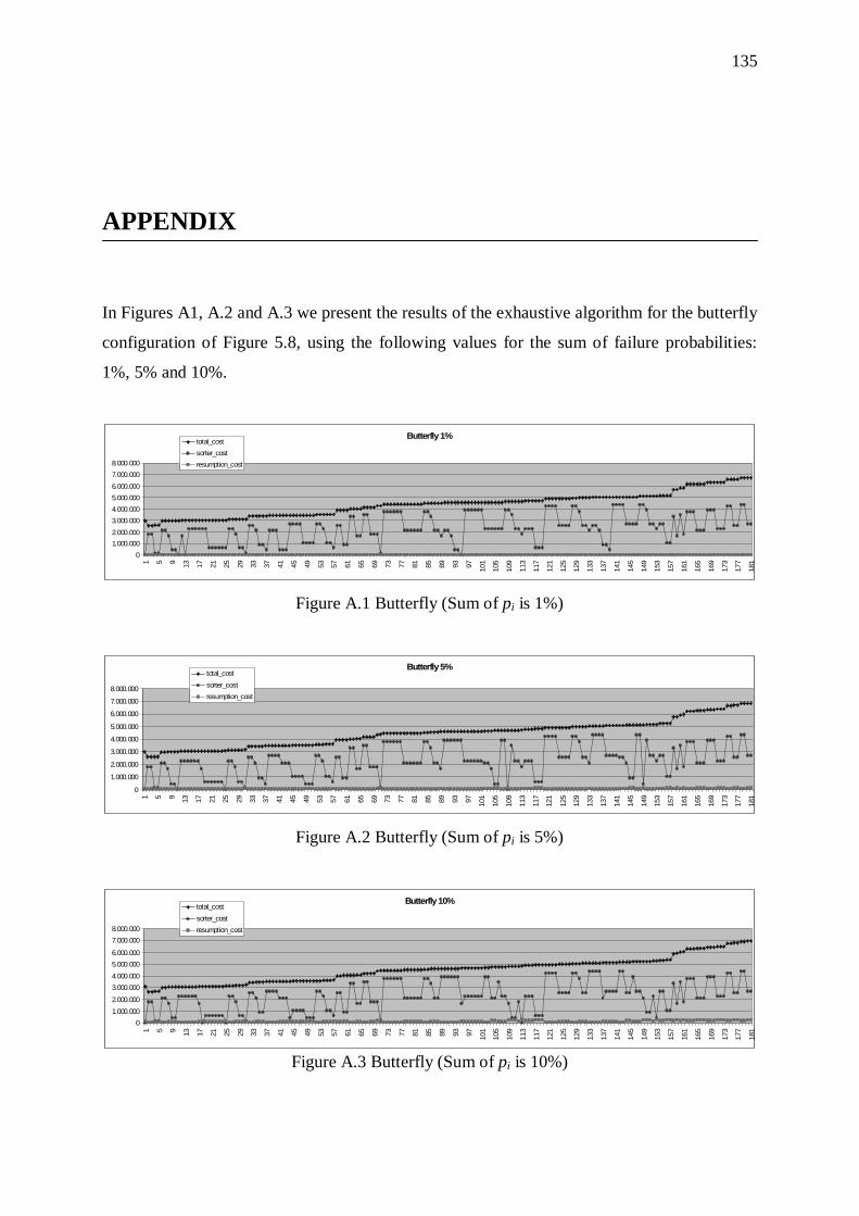
135

APPENDIX

In Figures A1, A.2 and A.3 we present the results of the exhaustive algorithm for the butterfly

configuration of Figure 5.8, using the following values for the sum of failure probabilities:

1%, 5% and 10%.

Butterfly 1%

0

1.000.000

2.000.000

3.000.000

4.000.000

5.000.000

6.000.000

7.000.000

8.000.000

1 5 9 13 17 21 25 29 33 37 41 45 49 53 57 61 65 69 73 77 81 85 89 93 97 101

105

109

113

117

121

125

129

133

137

141

145

149

153

157

161

165

169

173

177

181

total_cost

sorter_cost

resumption_cost

Figure A.1 Butterfly (Sum of pi is 1%)

Butterfly 5%

0

1.000.000

2.000.000

3.000.000

4.000.000

5.000.000

6.000.000

7.000.000

8.000.000

1 5 9 13 17 21 25 29 33 37 41 45 49 53 57 61 65 69 73 77 81 85 89 93 97 101

105

109

113

117

121

125

129

133

137

141

145

149

153

157

161

165

169

173

177

181

total_cost

sorter_cost

resumption_cost

Figure A.2 Butterfly (Sum of pi is 5%)

Butterfly 10%

0

1.000.000

2.000.000

3.000.000

4.000.000

5.000.000

6.000.000

7.000.000

8.000.000

1 5 9 13 17 21 25 29 33 37 41 45 49 53 57 61 65 69 73 77 81 85 89 93 97 101

105

109

113

117

121

125

129

133

137

141

145

149

153

157

161

165

169

173

177

181

total_cost

sorter_cost

resumption_cost

Figure A.3 Butterfly (Sum of pi is 10%)

136

SHORT BIOGRAPHICAL SKETCH

Vasiliki Tziovara was born in Ioannina in 1979. She finished high school in 1997 and

obtained her degree from the Department of Computer Science of the University of Ioannina

in 2001. Vasiliki Tziovara has enrolled in the Graduate Program of the Computer Science

Department of the University of Ioannina as an MSc candidate in the academic year 2003 -

2004. During the first year of her studies in the Graduate Program of Computer Science, she

received a scholarship for her performance. Her research interests include Data Warehouses

and Extraction-Transformation-Loading (ETL) workflows. She is currently working as a

teacher in a public school in Metsovo.