Robust Scheduling for Real-Time and Non-Real-Time Traffic ...
Upload
jonathan-ramseyCategory
view
213download
0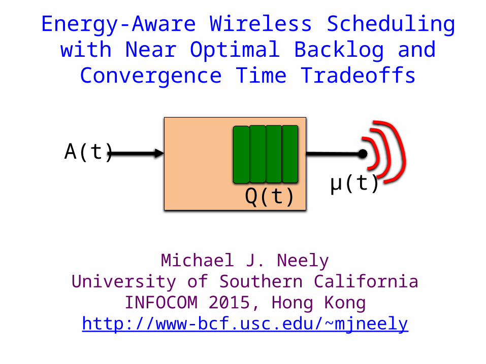
Energy-Aware Wireless Scheduling with Near Optimal Backlog and Convergence Time Tradeoffs
Michael J. NeelyUniversity of Southern California
INFOCOM 2015, Hong Konghttp://www-bcf.usc.edu/~mjneely
A(t)
Q(t)μ(t)
A(t)
Q(t)μ(t)
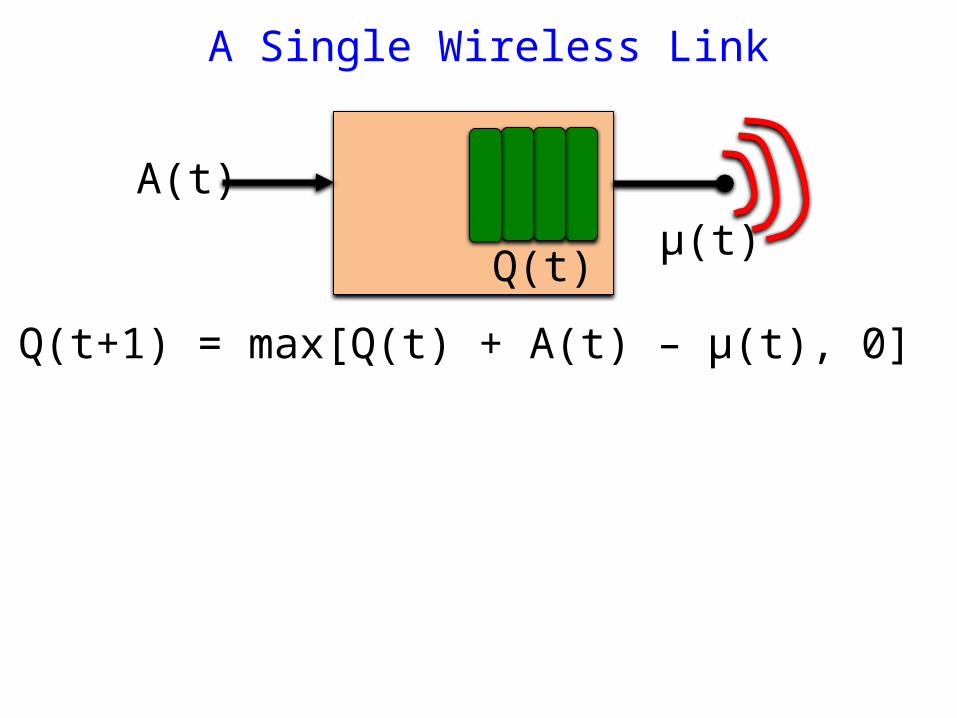
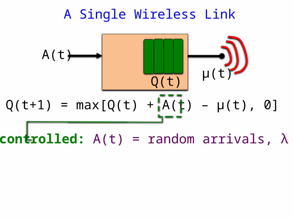
Q(t+1) = max[Q(t) + A(t) – μ(t), 0]
A Single Wireless Link
A(t)
Q(t)μ(t)
Q(t+1) = max[Q(t) + A(t) – μ(t), 0]
A Single Wireless Link
Uncontrolled: A(t) = random arrivals, λ
A(t)
Q(t)μ(t)
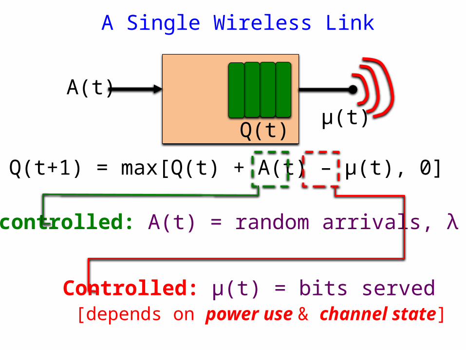
Q(t+1) = max[Q(t) + A(t) – μ(t), 0]
A Single Wireless Link
Uncontrolled: A(t) = random arrivals, λ
Controlled: μ(t) = bits served [depends on power use & channel state]
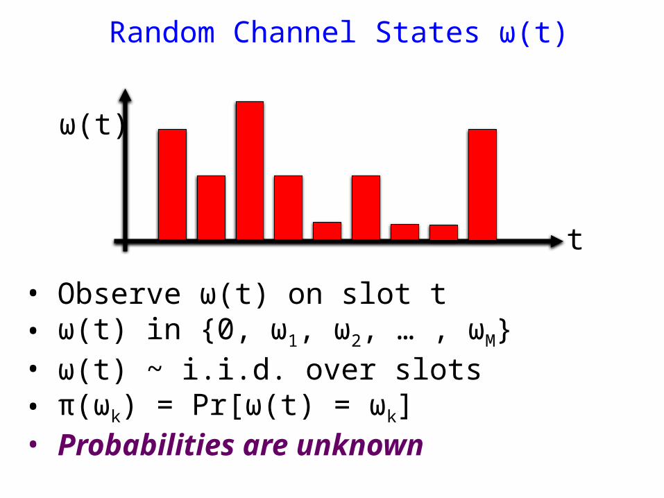
Random Channel States ω(t)
t
ω(t)
• Observe ω(t) on slot t• ω(t) in {0, ω1, ω2, … , ωM}• ω(t) ~ i.i.d. over slots • π(ωk) = Pr[ω(t) = ωk]• Probabilities are unknown
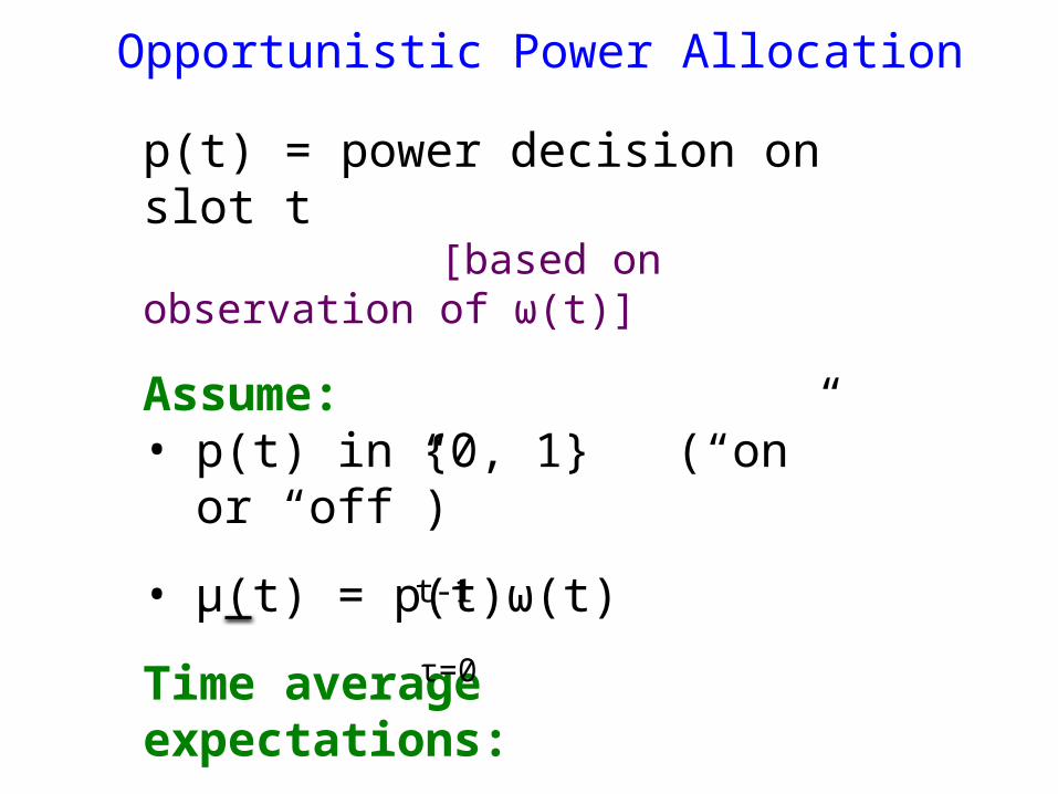
Opportunistic Power Allocation
p(t) = power decision on slot t [based on observation of ω(t)]
Assume: • p(t) in {0, 1} (“on” or “off”)
• μ(t) = p(t)ω(t)
Time average expectations:
p(t) = (1/t) ∑ E[ p(τ) ]
τ=0
t-1
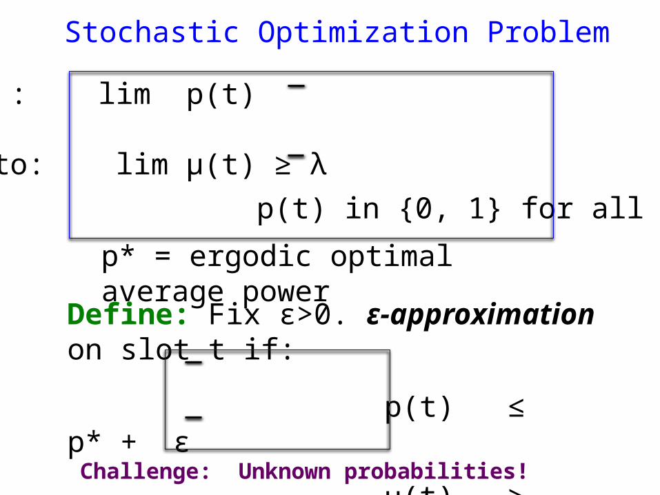
Stochastic Optimization Problem
Minimize : lim p(t)
Subject to: lim μ(t) ≥ λ p(t) in {0, 1} for all slots t
p* = ergodic optimal average power
Define: Fix ε>0. ε-approximation on slot t if:
p(t) ≤ p* + ε
μ(t) ≥ λ - εChallenge: Unknown probabilities!
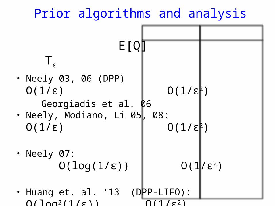
Prior algorithms and analysis E[Q] Tε
• Neely 03, 06 (DPP) O(1/ε) O(1/ε2) Georgiadis et al. 06• Neely, Modiano, Li 05, 08: O(1/ε) O(1/ε2)
• Neely 07: O(log(1/ε)) O(1/ε2)
• Huang et. al. ‘13 (DPP-LIFO): O(log2(1/ε)) O(1/ε2)
• Li, Li, Eryilmaz ‘13, ’15: O(1/ε) O(1/ε2) (additional sample path results)
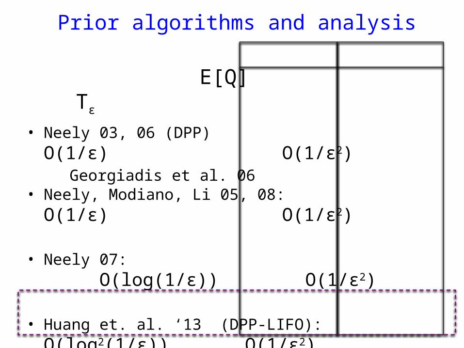
Prior algorithms and analysis E[Q] Tε
• Neely 03, 06 (DPP) O(1/ε) O(1/ε2) Georgiadis et al. 06• Neely, Modiano, Li 05, 08: O(1/ε) O(1/ε2)
• Neely 07: O(log(1/ε)) O(1/ε2)
• Huang et. al. ‘13 (DPP-LIFO): O(log2(1/ε)) O(1/ε2)
• Li, Li, Eryilmaz ‘13, ’15: O(1/ε) O(1/ε2) (additional sample path results)
• Huang et al. ’14: O(1/ε2/3) O(1/ε1+2/3)
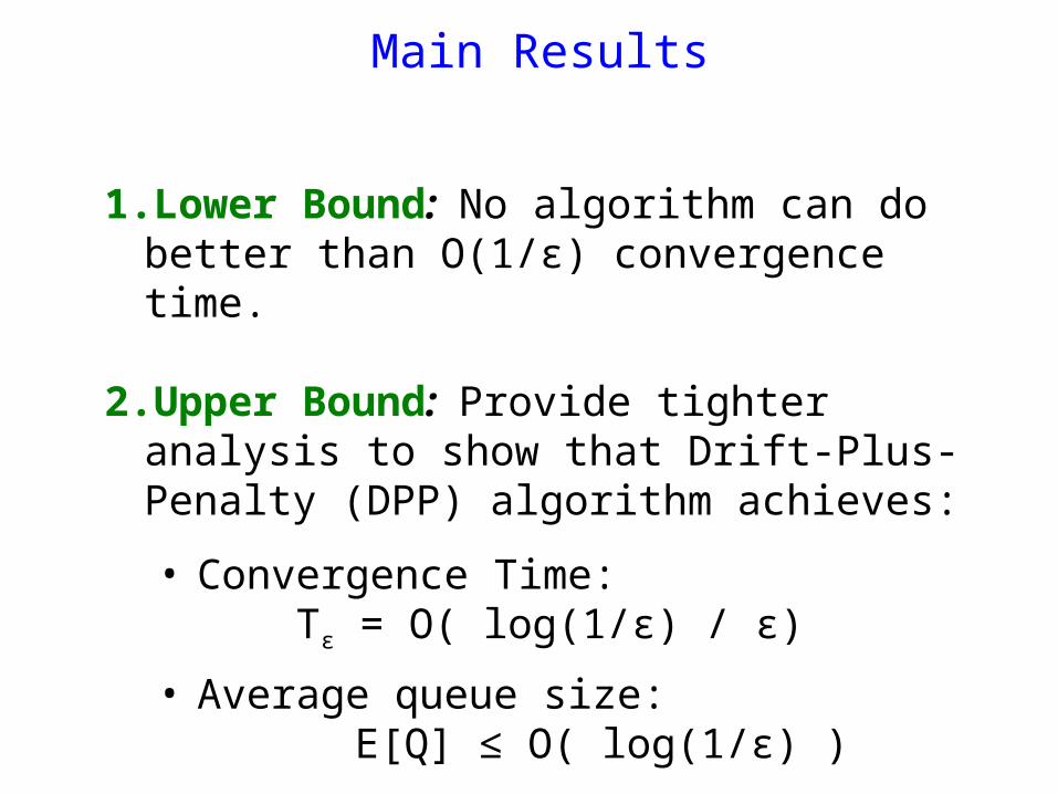
Main Results
1. Lower Bound: No algorithm can do better than O(1/ε) convergence time.
2. Upper Bound: Provide tighter analysis to show that Drift-Plus-Penalty (DPP) algorithm achieves:
• Convergence Time: Tε = O( log(1/ε) / ε)
• Average queue size: E[Q] ≤ O( log(1/ε) )
Part 1: Ω(1/ε) Lower Bound for all Algorithms
Example system:• ω(t) in {1, 2, 3} • Pr[ω(t) = 3], Pr[ω(t) = 2], Pr[ω(t) = 1] unknown.
Proof methodology: • Case 1: Pr[ transmit | ω(0) = 2 ] > ½.
o Assume Pr[ω(t) = 3] = Pr[ω(t) = 2] = ½.o Optimally compensate for mistake on slot 0.
• Case 2: Pr[ transmit | ω(0) = 2 ] ≤ ½.o Assume different probabilities.o Optimally compensate for mistake on slot 0.
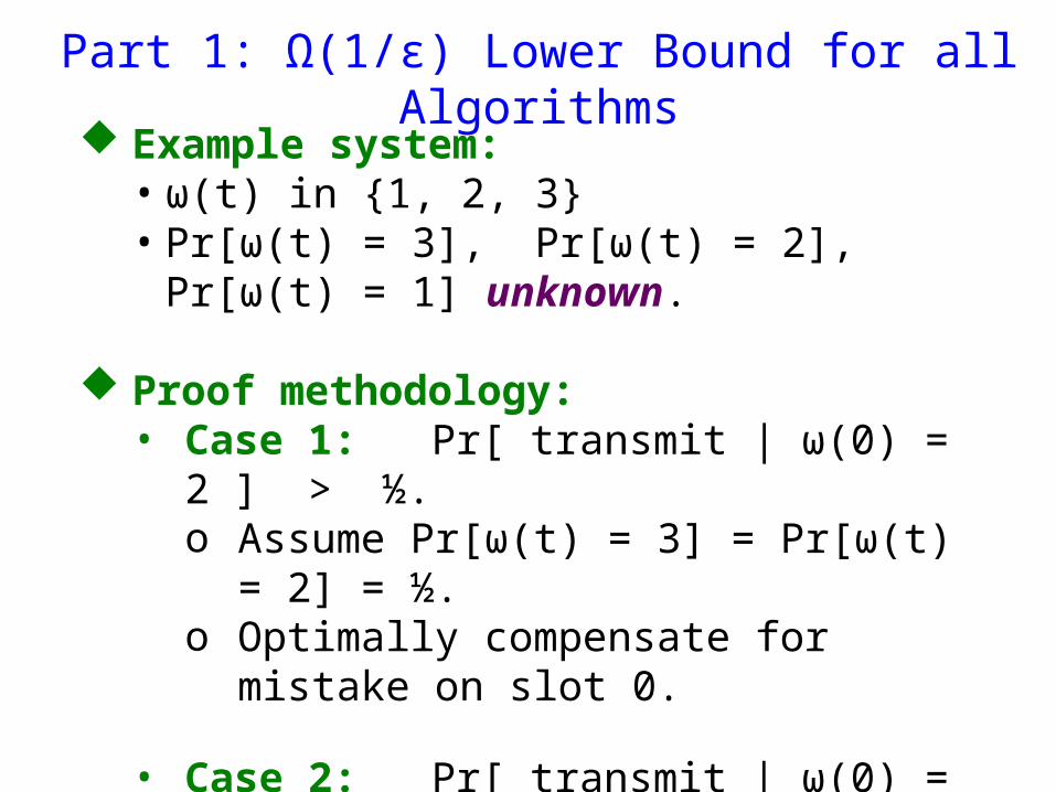
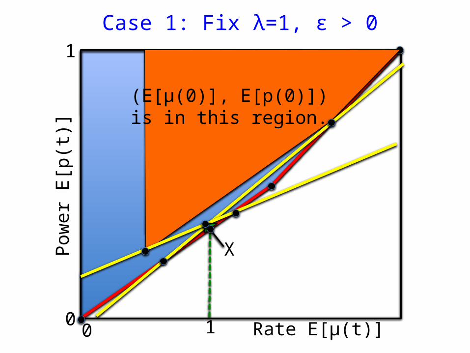
Case 1: Fix λ=1, ε > 0
Rate E[μ(t)]
Pow
er E
[p(t
)]
X
100
1
h(μ) curve
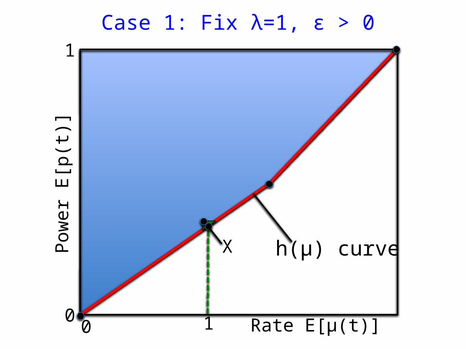
Case 1: Fix λ=1, ε > 0
Rate E[μ(t)]
Pow
er E
[p(t
)]
A
X
100
1
(E[μ(0)], E[p(0)]) is in this region.
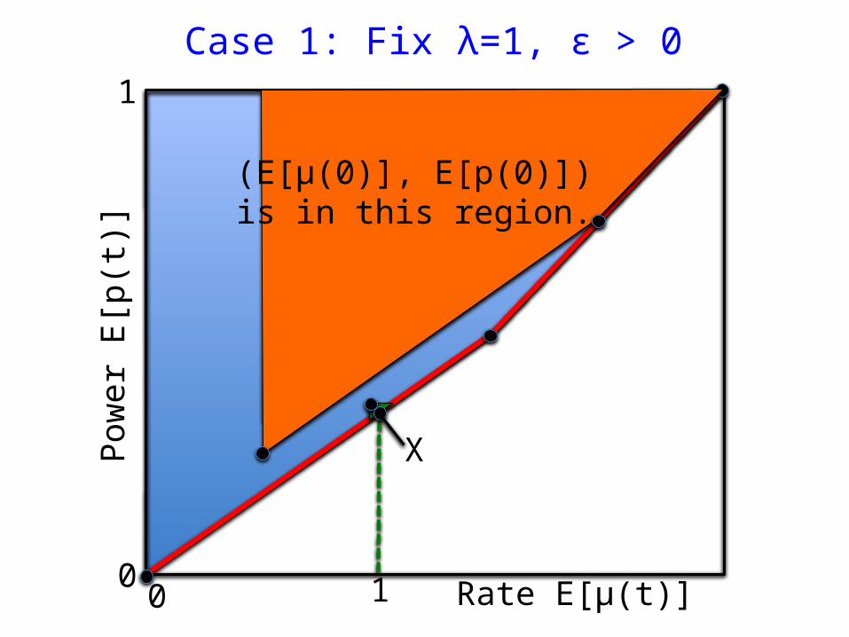
Case 1: Fix λ=1, ε > 0
Rate E[μ(t)]
Pow
er E
[p(t
)]
A
X
100
1
(E[μ(0)], E[p(0)]) is in this region.
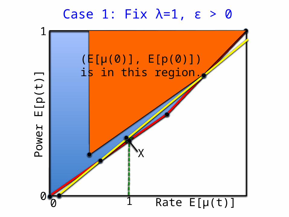
Case 1: Fix λ=1, ε > 0
Rate E[μ(t)]
Pow
er E
[p(t
)]
A
X
100
1
(E[μ(0)], E[p(0)]) is in this region.
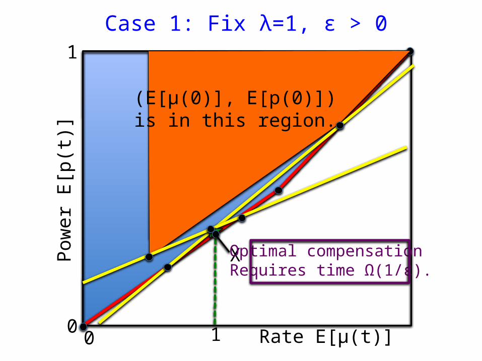
Case 1: Fix λ=1, ε > 0
Rate E[μ(t)]
Pow
er E
[p(t
)]
A
100
1
(E[μ(0)], E[p(0)]) is in this region.
X Optimal compensationRequires time Ω(1/ε).
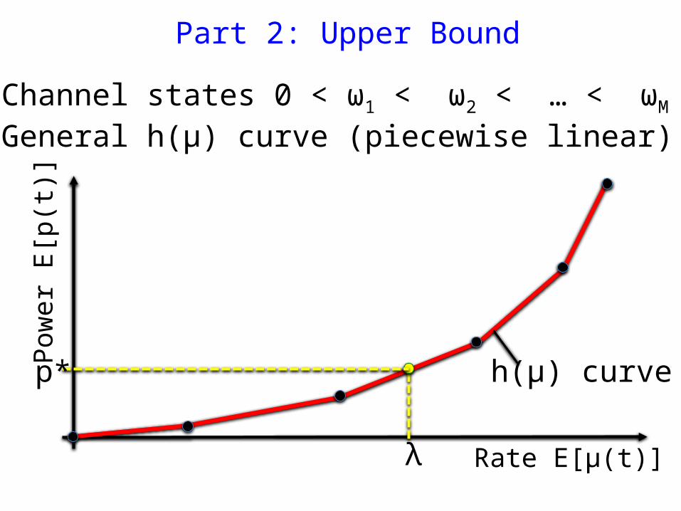
Part 2: Upper Bound
• Channel states 0 < ω1 < ω2 < … < ωM
• General h(μ) curve (piecewise linear)
Pow
er E
[p(t
)]
Rate E[μ(t)]λ
h(μ) curvep*
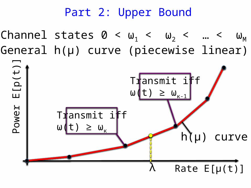
Part 2: Upper Bound
• Channel states 0 < ω1 < ω2 < … < ωM
• General h(μ) curve (piecewise linear)
Rate E[μ(t)]λ
h(μ) curve
Transmit iffω(t) ≥ ωκ-1
Transmit iffω(t) ≥ ωκ
Pow
er E
[p(t
)]
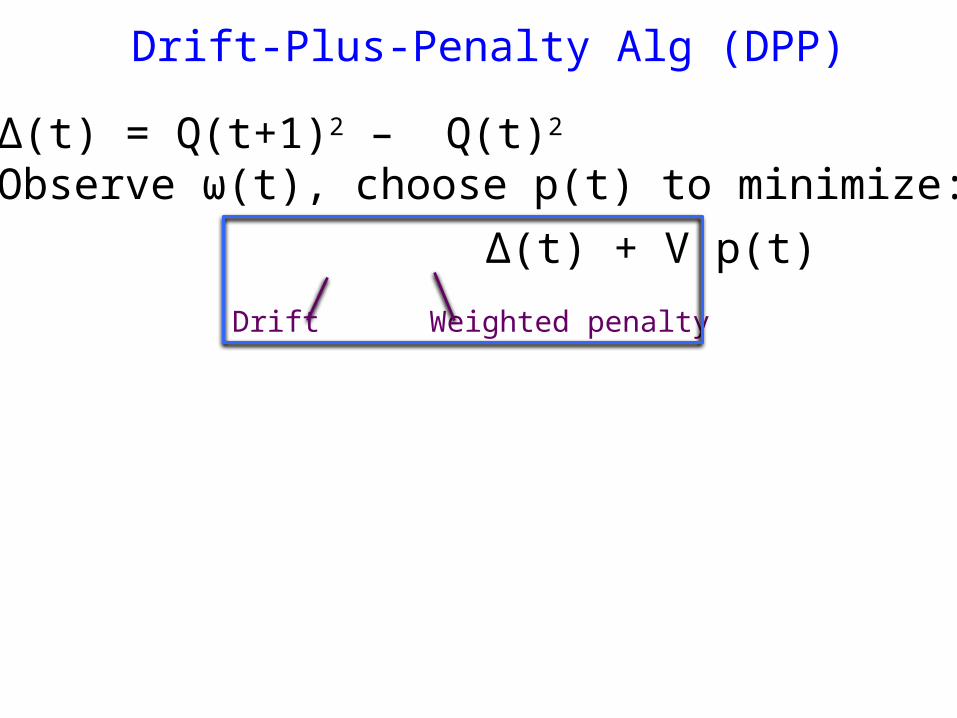
Drift-Plus-Penalty Alg (DPP)
• Δ(t) = Q(t+1)2 – Q(t)2
• Observe ω(t), choose p(t) to minimize: Δ(t) + V p(t)
Weighted penaltyDrift
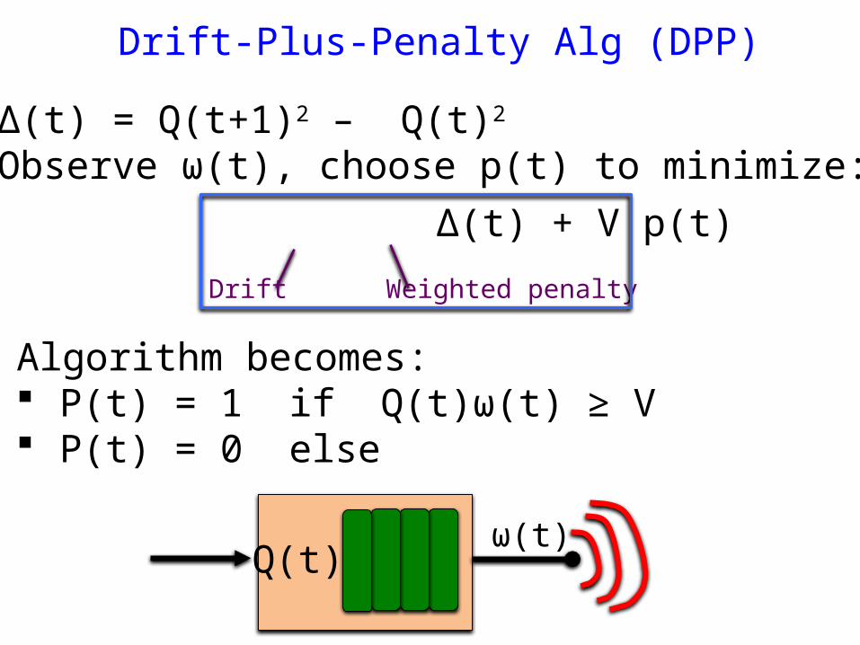
Drift-Plus-Penalty Alg (DPP)
• Δ(t) = Q(t+1)2 – Q(t)2
• Observe ω(t), choose p(t) to minimize: Δ(t) + V p(t)
Weighted penaltyDrift
• Algorithm becomes: P(t) = 1 if Q(t)ω(t) ≥ V P(t) = 0 else
Q(t)ω(t)
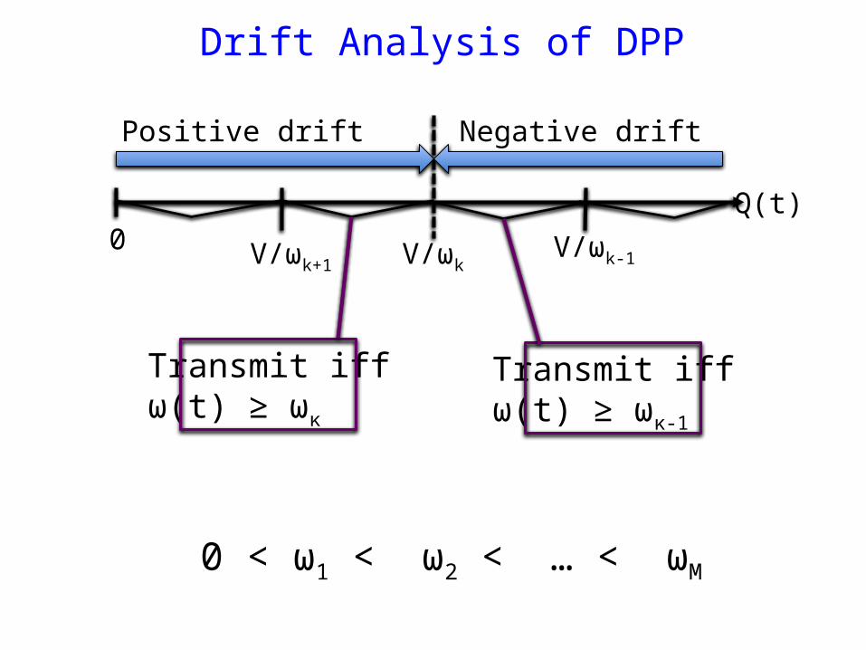
Drift Analysis of DPP
Transmit iffω(t) ≥ ωκ-1
Transmit iffω(t) ≥ ωκ
V/ωkV/ωk+1V/ωk-1
0Q(t)
Positive drift Negative drift
0 < ω1 < ω2 < … < ωM
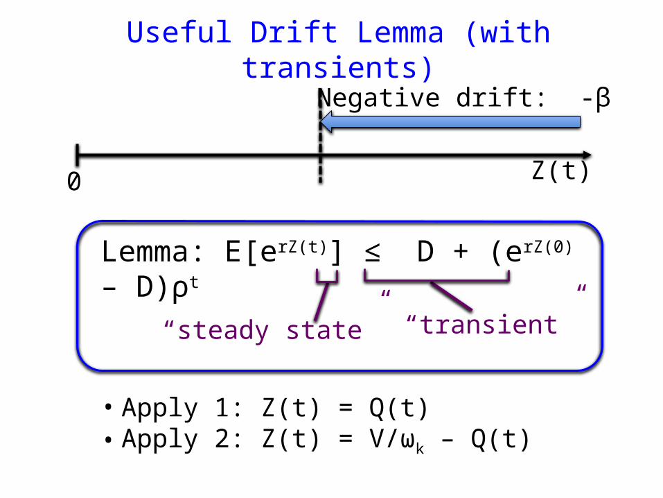
Useful Drift Lemma (with transients)
Z(t)
Negative drift: -β
0
Lemma: E[erZ(t)] ≤ D + (erZ(0) – D)ρt
“steady state” “transient”
• Apply 1: Z(t) = Q(t)• Apply 2: Z(t) = V/ωk – Q(t)
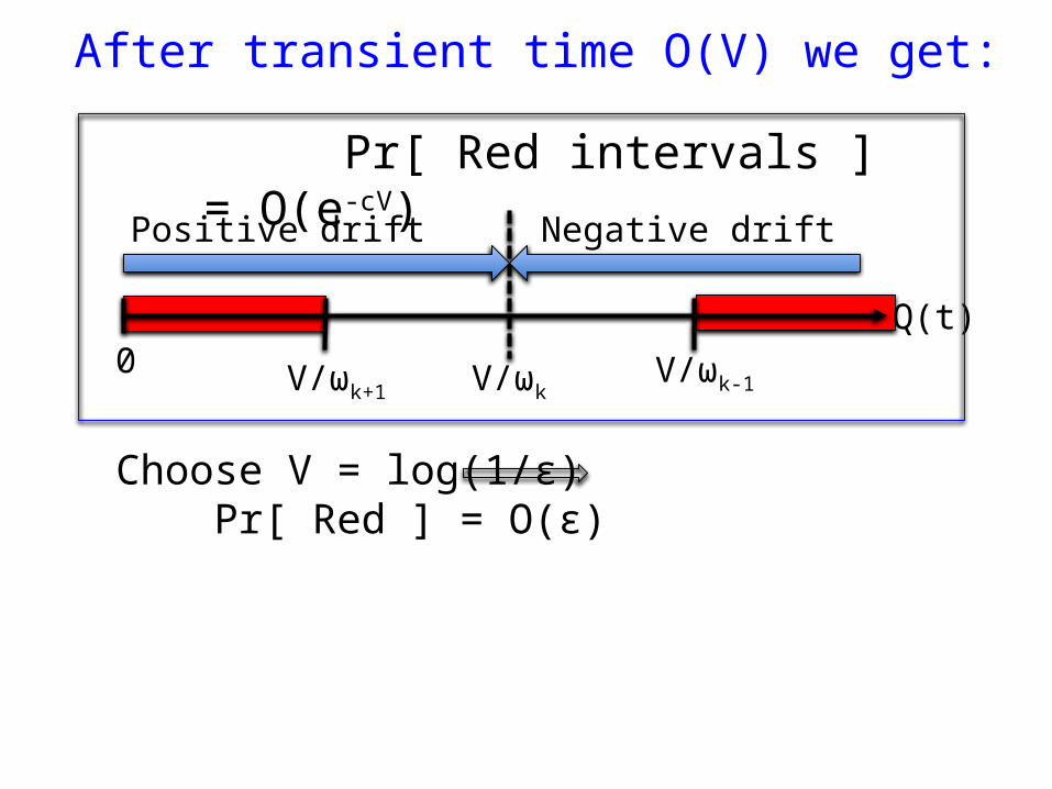
After transient time O(V) we get:
V/ωkV/ωk+1V/ωk-1
0Q(t)
Positive drift Negative drift
Pr[ Red intervals ] = O(e-cV)
Choose V = log(1/ε) Pr[ Red ] = O(ε)
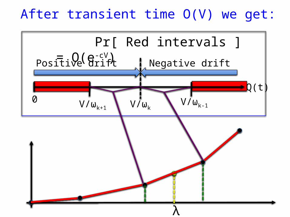
After transient time O(V) we get:
V/ωkV/ωk+1V/ωk-1
0Q(t)
Positive drift Negative drift
Pr[ Red intervals ] = O(e-cV)
λ
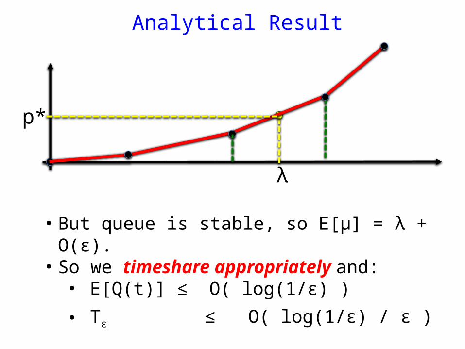
Analytical Result
λ
• But queue is stable, so E[μ] = λ + O(ε).• So we timeshare appropriately and: • E[Q(t)] ≤ O( log(1/ε) )
• Tε ≤ O( log(1/ε) / ε )
p*
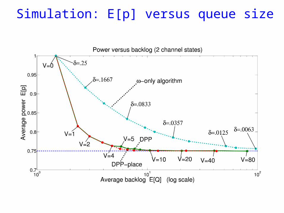
Simulation: E[p] versus queue size
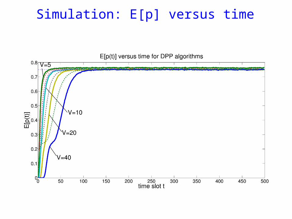
Simulation: E[p] versus time
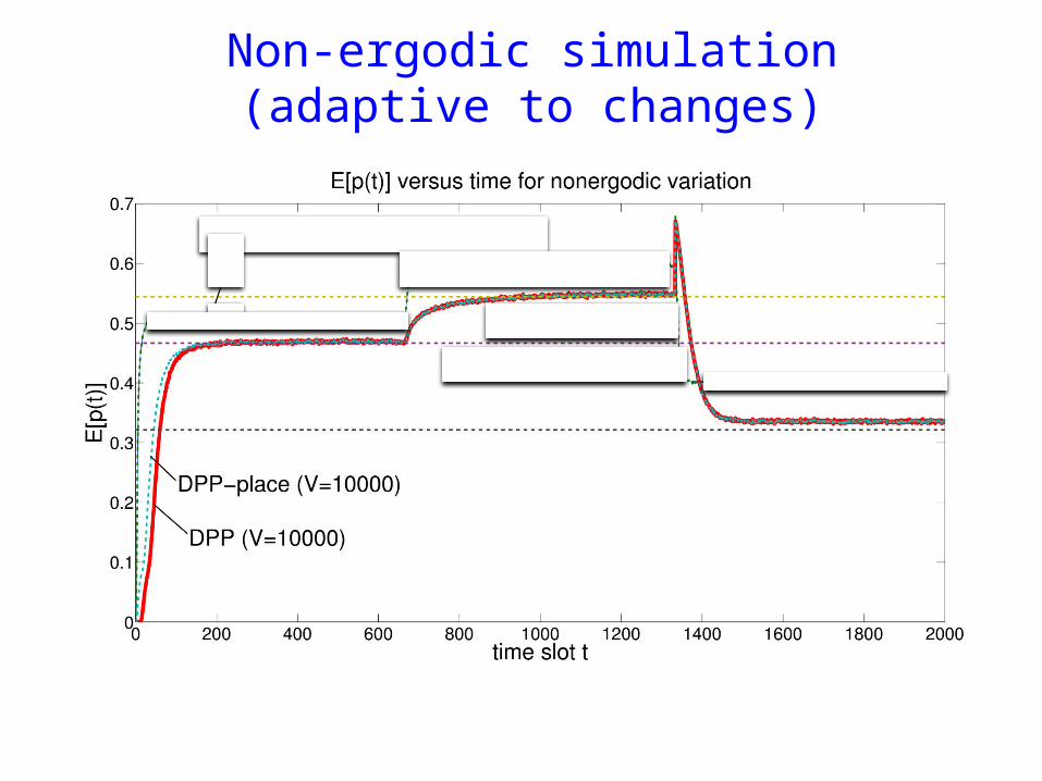
Non-ergodic simulation(adaptive to changes)
Conclusions
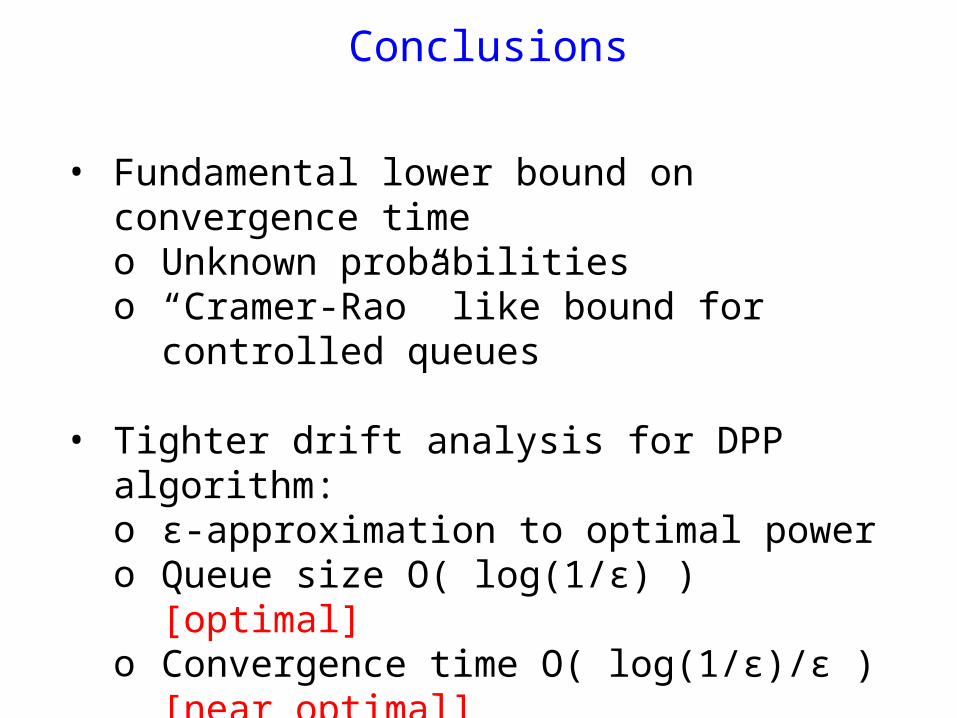
• Fundamental lower bound on convergence timeo Unknown probabilitieso “Cramer-Rao” like bound for controlled queues
• Tighter drift analysis for DPP algorithm: o ε-approximation to optimal powero Queue size O( log(1/ε) ) [optimal]o Convergence time O( log(1/ε)/ε ) [near optimal]