INSTITUTE OF PHYSICS PUBLISHING PHYSICS IN MEDICINE AND BIOLOGY

Phys. Med. Biol. 49 (2004) 2129–2143 PII: S0031-9155(04)69762-4

On two versions of a 3π algorithm for spiral CT

Alexander Katsevich

Department of Mathematics, University of Central Florida, Orlando, FL 32816-1364, USA

E-mail: akatsevi@pegasus.cc.ucf.edu

Received 1 October 2003Published 19 May 2004Online at stacks.iop.org/PMB/49/2129DOI: 10.1088/0031-9155/49/11/001

AbstractA 3π algorithm is obtained in which all the derivatives are confined to a detectorarray. Distance weighting of backprojection coefficients of the algorithmis studied. A numerical experiment indicates that avoiding differentiationalong the source trajectory improves spatial resolution. Another numericalexperiment shows that the terms depending on the non-standard distanceweighting 1/|x − y(s)| can no longer be ignored.

1. Introduction

Using redundant data is important in spiral CT. It leads to the reduction of motion and samplingartefacts, efficient use of the applied dose, etc (Bontus et al 2001, Kohler et al 2002). InKatsevich (2003, 2004) a theoretically exact shift-invariant FBP-type algorithm for spiral CTwas proposed that allows one to use redundant data. A closely related quasi-exact algorithmwas proposed in Bontus et al (2003a, 2003b). The algorithms operate in the 3π mode andrequire a detector array, which is about three times as large as that required for 1π algorithms(see, e.g., Proksa et al (2000), Katsevich (2002)). This aspect of 3π algorithms is veryimportant in medical applications of CT. The reason is that as the number of detector rows andgantry rotation speed continue to increase, 1π algorithms will reach their limitation. Considera next generation 64 slice scanner, whose gantry makes three revolutions per second. Usingtable 1 of Noo et al (2003) we see that maximum detector utilization with a 1π algorithm isachieved when the table feed equals 6.58 cm per rotation. This translates into the table speedof about 20 cm s−1, which is too high for many patients. 3π algorithms will allow one to slowthe table down, but still maintain high detector utilization.

Similarly to the 1π case (see Katsevich 2002), 3π algorithms also admit two versions.Version 1 requires differentiation along the source trajectory. In version 2 all derivatives areconfined to the detector array. Since detector sampling is usually much finer than samplingof the source trajectory, it is reasonable to expect that the second version will provide betterspatial resolution. The main purpose of this paper is to derive the second version of the 3π

algorithm of Katsevich (2004) and to investigate how the resulting backprojection coefficients

0031-9155/04/112129+15$30.00 © 2004 IOP Publishing Ltd Printed in the UK 2129

2130 A Katsevich

depend on distance weighting. We show that similarly to the 1π case two weights are neededto backproject the filtered cone beam projections: 1/|x − y(s)| and 1/|x − y(s)|2. Here|x − y(s)| denotes the distance from the focal point y(s) to the reconstruction point x. Apreliminary numerical experiment presented in the paper indicates that the second version ofthe 3π algorithm provides better spatial resolution (at least, in the current implementation).Another numerical experiment shows that, as opposed to the 1π case (see Katsevich et al2003), the terms depending on the non-standard distance weighting 1/|x −y(s)| can no longerbe ignored.

Note that the numerical implementations of the two versions of the 3π algorithm havenot been optimized. In particular, all convolutions are performed with respect to the polarangle γ . This is the most obvious approach, but its downside is the need for excessiveinterpolation, which results in reduced spatial resolution. Recently, F Noo, J Pack andD Heuscher proposed a very efficient and accurate method of implementing version 1 ofthe 1π algorithm of Katsevich (2002) (see Noo et al 2003). One of the features in theirapproach is that the convolutions are performed with respect to a ‘native’ coordinate on thedetector. This and other improvements resulted in a significant increase in efficiency, spatialresolution and overall image quality. It is quite clear that most of these ideas can be applied toversion 1 of the 3π algorithm. The application of the ideas to version 2 of the 3π algorithmis more challenging. Thus, finding optimal implementations of the two versions of the 3π

algorithm and a detailed investigation of their numerical performance will be the subject offuture research. The purpose of the numerical experiments presented in this paper is only todemonstrate that version 2 of the 3π algorithm works and, given comparable implementations,appears to provide better spatial resolution than version 1.

2. The 3π algorithm

First we introduce the necessary notations. Let

C := {y ∈ R3 : y1 = R cos(s), y2 = R sin(s), y3 = s(h/2π), s ∈ R} h > 0 (2.1)

be a spiral, and U be an open set strictly inside the spiral:

U ⊂ {x ∈ R

3 : x21 + x2

2 < r2}

0 < r < R. (2.2)

S2 is the unit sphere in R3, and

Df (y, β) :=∫ ∞

0f (y + βt) dt β ∈ S2 (2.3)

β(s, x) := x − y(s)

|x − y(s)| x ∈ U, s ∈ R (2.4)

that is Df (y, β) is the cone beam transform of f . Also, y(s) := dy/ds. For β ∈ S2, β⊥

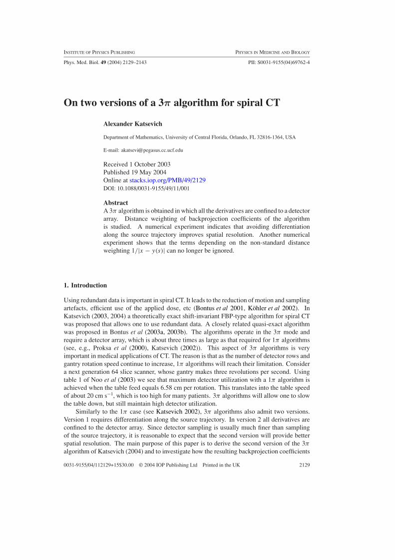
denotes the great circle {α ∈ S2 : α · β = 0}. In what follows it is assumed that r/R < 0.618.Suppose that the x-ray source is fixed at y(s0) for some s0 ∈ R. Since the detector array

rotates together with the source, the detector plane depends on s0 and is denoted by DP(s0).It is assumed that DP(s0) is parallel to the axis of the spiral and is tangent to the cylindery2

1 + y22 = R2 (cf (2.1)) at the point opposite to the source. Thus, the distance between y(s0)

and the detector plane is 2R (see figure 1). Introduce coordinates in the detector plane asfollows. Let the d1-axis be perpendicular to the axis of the spiral, the d2-axis be parallel to itand the origin coincide with the projection of y(s0). Project stereographically the upper and

On two versions of a 3π algorithm for spiral CT 2131

Detector plane DP(s0)

y(s0)

j3

rotationaxis

C

d1

d2

2RΓ1

Γ−1

Γ2

Γ−2

Figure 1. Stereographic projection of the spiral onto the detector plane.

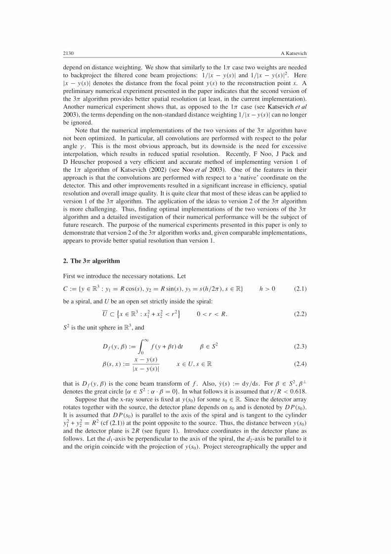
Figure 2. Detector plane with various projections and important lines shown.

lower turns of the spiral onto the detector plane as shown in figure 1. This gives the followingparametric curves:

d1(s) = 2Rsin(s − s0)

1 − cos(s − s0)d2(s) = h

π

s − s0

1 − cos(s − s0)

ρ + 2π(j − 1) � s − s0 � 2πj − ρ j � 1 or

ρ + 2πj � s − s0 � 2π(j + 1) − ρ j � −1

(2.5)

where ρ is determined by radius of support of the object: ρ = 2 cos−1(r/R) (cf (2.2)).These curves are denoted by �j , j = ±1,±2, . . . (see figure 2). L0 is the projection of thespiral tangent, and Lcr

±2 are lines parallel to L0 and tangent to �±2, respectively. Lcr−1,1 is

the line tangent to both �1 and �−1. The quantity � is determined as the unique solution oftan � = �,π < � < 3π/2 (cf Katsevich 2004).

Let x denote the projection of x. Sometimes we will write x(s) to emphasize that thelocation of x on DP(s) depends on the source position y(s). As is well known, x(s) is between

2132 A Katsevich

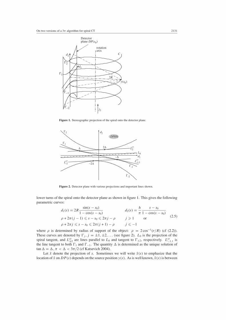
Figure 3. Family L0 of filtering lines parallel to the spiral tangent (left-hand panel) and family L1of filtering lines tangent to �±1 (right-hand panel).

�−1 and �1 if and only if s ∈ I 1π (x). Here I 1π (x) := [b1π (x), t1π (x)] is the 1π parametricinterval of x. The region on the detector bounded by �−1 and �1 is known in the literature as 1π

or Tam–Danielsson window (Tam 1995, Tam et al 1998, Danielsson et al 1997). In a similarfashion, the region between �−2 and �2 is called the 3π window (Katsevich 2004). Let I 3π (x)

be the parametric interval such that x(s) is inside the 3π window if and only if s ∈ I 3π (x). Thecorresponding section of the spiral is denoted by C3π (x). It is shown in Proksa et al (2000)and Katsevich (2004) that I 3π (x) is either a single interval I 3π (x) = [

b3π1 , t3π

1

]or consists of

three subintervals I 3π (x) = ∪3i=1

[b3π

i , t3πi

](here we use the notation slightly different from

that of Katsevich (2004).Now define three families of filtering lines. The first family, which consists of lines

parallel to L0, is denoted by L0 (see figure 3, left-hand panel). The second family, whichconsists of lines tangent to �±1, is denoted by L1 (see figure 3, right-hand panel).

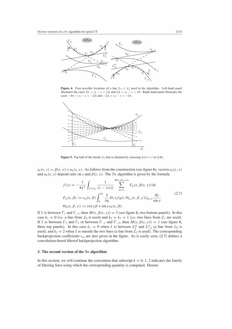
Let ψ(t) be any smooth function with the properties ψ(0) = 0, ψ ′(t) > 0, t ∈ R. Definethe family of lines L2 by requesting that any given L ∈ L2 has three points of intersectionwith �±1 ∪ �±2: s1, s2, s3, and these points satisfy

{s1 − s = ψ(s3 − s2) s + 2π < s3 < s + 4π

s2 − s3 = ψ(s − s1) s − 4π < s3 < s − 2π.(2.6)

The requirement that s1, s2, s3 belong to a line reduces the number of degrees of freedom fromthree to two. Equation (2.6) further reduces this number to one. Consequently, the lines L ∈ L2

can be parametrized by only one parameter. One can use, for example, s3, 2π < |s3| < 4π .The location of the intersection points depends on where s3 is and is illustrated in figure 4.Top half of the family L2 that is obtained by choosing ψ(t) = t in (2.6) is shown in figure 5.One has that x → Lcr

2 implies L → Lcr2 . Similarly, x → Lcr

−2 implies L → Lcr−2.

Figure 6 summarizes which filtering lines are used depending on where x is inside the 3π

window, provided that x is above L0. If x is below L0, then the filtering lines are obtainedfrom figure 6 using symmetry about the origin.

Given x and a source position y(s), s ∈ I 3π (x), find a filtering line L ∈ Lk, k = 0, 1, 2,containing x. The point and line determine the plane (s, x). Let uk(s, x) be the unit vectorperpendicular to (s, x) and pointing up (i.e. in the direction of the spiral motion). Denote

On two versions of a 3π algorithm for spiral CT 2133

Figure 4. Four possible locations of a line L2 ∈ L2 used in the algorithm. Left-hand panelillustrates the cases 2π < s3 − s < 2� and 2� < s3 − s < 4π . Right-hand panel illustrates thecases −4π < s3 − s < −2� and −2� < s3 − s < −2π .

Figure 5. Top half of the family L2 that is obtained by choosing ψ(t) = t in (2.6).

ek(s, x) = β(s, x)×uk(s, x). As follows from the construction (see figure 6), vectors ek(s, x)

and uk(s, x) depend only on s and β(s, x). The 3π algorithm is given by the formula

f (x) = − 1

4π2

∫I 3π (x)

1

|x − y(s)|M(s,β(s,x))∑

m=1

Fm(s, β(s, x)) ds

Fm(s, β) := cm(s, β)

∫ 2π

0

∂

∂qDf (y(q),�km

(s, β, γ ))|q=s

dγ

sin γ

�k(s, β, γ ) := cos γβ + sin γ ek(s, β).

(2.7)

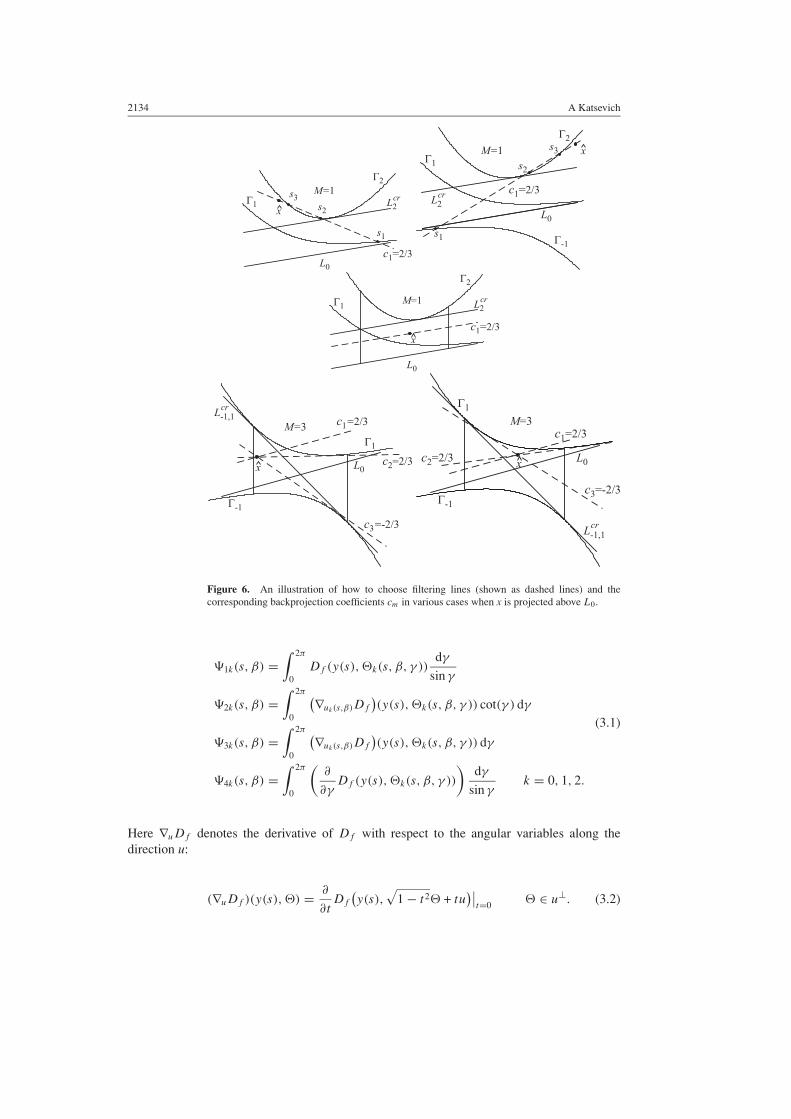
If x is between �1 and �−1, then M(s, β(s, x)) = 3 (see figure 6, two bottom panels). In thiscase k1 = 0 (i.e. a line from L0 is used) and k2 = k3 = 1 (i.e. two lines from L1 are used).If x is between �1 and �2 or between �−1 and �−2, then M(s, β(s, x)) = 1 (see figure 6,three top panels). In this case k1 = 0 when x is between Lcr

2 and Lcr−2 (a line from L0 is

used), and k1 = 2 when x is outside the two lines (a line from L2 is used). The correspondingbackprojection coefficients cm are also given in the figure. As is easily seen, (2.7) defines aconvolution-based filtered backprojection algorithm.

3. The second version of the 3π algorithm

In this section, we will continue the convention that subscript k = 0, 1, 2 indicates the familyof filtering lines using which the corresponding quantity is computed. Denote

2134 A Katsevich

Figure 6. An illustration of how to choose filtering lines (shown as dashed lines) and thecorresponding backprojection coefficients cm in various cases when x is projected above L0.

�1k(s, β) =∫ 2π

0Df (y(s),�k(s, β, γ ))

dγ

sin γ

�2k(s, β) =∫ 2π

0

(∇uk(s,β)Df

)(y(s),�k(s, β, γ )) cot(γ ) dγ

�3k(s, β) =∫ 2π

0

(∇uk(s,β)Df

)(y(s),�k(s, β, γ )) dγ

�4k(s, β) =∫ 2π

0

(∂

∂γDf (y(s),�k(s, β, γ ))

)dγ

sin γk = 0, 1, 2.

(3.1)

Here ∇uDf denotes the derivative of Df with respect to the angular variables along thedirection u:

(∇uDf )(y(s),�) = ∂

∂tDf

(y(s),

√1 − t2� + tu

)∣∣t=0 � ∈ u⊥. (3.2)

On two versions of a 3π algorithm for spiral CT 2135

Denote also

µ1k(s, x) = ∂

∂s

1

|x − y(s)| µ2k(s, x) = β ′s(s, x) · uk(s, x)

|x − y(s)|µ3k(s, x) = (ek)

′s(s, x) · uk(s, x)

|x − y(s)| µ4k(s, x) = β ′s(s, x) · ek(s, x)

|x − y(s)| .

(3.3)

Here β ′s = ∂β/∂s and e′

s = ∂e/∂s.Integrating by parts with respect to s in (2.7) similarly to Katsevich (2002), we obtain

an inversion formula in which all the derivatives are performed with respect to the angularvariables.

f (x) = − 1

4π2

N3π (x)∑i=1

c2(s, β)�12(s, β)

|x − y(s)|

∣∣∣∣∣∣s=t3π

i (x)

s=b3πi (x)

−∫

I 3π (x)

M(s,β)∑m=1

cm(s, β)

4∑j=1

µjkm(s, x)�jkm

(s, β) ds

β = β(s, x)

(3.4)

where N3π (x) equals either 1 or 3, depending on how many subintervals I 3π (x) consists of.Let us recall that (3.4) is obtained by substituting the identity

∂

∂qDf (y(q),�(s, x, γ ))|q=s = ∂

∂sDf (y(s),�(s, x, γ )) − ∂

∂qDf (y(s),�(q, x, γ ))|q=s

(3.5)

into (2.7) and integrating the first term by parts with respect to s. To avoid differentiating adiscontinuous function, we represent the integral over I 3π (x) as a sum of integrals over smallersubsets of I 3π (x) such that all functions in (2.7) are continuous inside these subsets. Byconstruction, a discontinuity may occur when one of the following happens: x(s), s ∈ I 3π (x),intersects �±1, L

cr±2, L

cr−1,1 or �±2.

Consider now each of these cases. When x(s) → �±1 from inside of the 1π window,the two filtering lines L ∈ L1 through x(s) approach each other. Since the correspondingbackprojection coefficients are c2 = 2/3 and c3 = −2/3, the contributions of these filteringlines cancel each other when x(s) ∈ �±1. Consequently, the corresponding boundary termthat arises after integration by parts equals zero.

When x(s) intersects Lcr2 , we have to switch from one family of filtering lines to another

(say, from L0 to L2). However, both the limiting filtering lines and the correspondingbackprojection coefficients are the same regardless of the direction from which x(s) approachesLcr

2 . Let s0 be such that x(s0) ∈ Lcr2 . Our argument implies that the boundary terms which

arise after integration by parts on each side of s0 cancel each other. The same cancellationoccurs when x(s) intersects Lcr

−2.When x(s) intersects Lcr

−1,1, the tangency point of one of the two filtering lines L ∈ L1

experiences a jump. As before, the limiting filtering lines and the backprojection coefficientsc3 (see two bottom panels of figure 6) are the same regardless of the direction from which x(s)

approaches Lcr−1,1. Consequently, no boundary terms arise from this discontinuity as well.

Thus, boundary terms arise only when x(s) intersects �±2, i.e. when s coincides withthe boundary of I 3π (x). Because of this analysis, we can assume in what follows that allquantities are locally continuous.

2136 A Katsevich

Denote for convenience L := |x−y(s)|. For future references we state here the followinguseful formulae:

µ1k = ∂

∂s

1

|x − y(s)| = β · y(s)

L2(3.6)

and

β ′s(s, x) = ∂

∂s

x − y(s)

|x − y(s)| = −y(s) + β(β · y(s))

L. (3.7)

Here and in what follows β = β(s, x). In this section we omit the subscript of ek and uk ,because it will be clear from the context which family of filtering lines is discussed. From(3.3), µ1k is independent of k and is determined using (3.6).

The remaining backprojection coefficients for lines L ∈ L0 are easy to find. Since thefiltering direction is parallel to the spiral tangent, we get

u(s, x) = y(s) × β

|y(s) × β| e = β × u = y(s) − β(β · y(s))

|y(s) × β| . (3.8)

Using (3.7) and (3.8) we compute

β ′s · u = 0 β ′

s · e = −|y(s)|2 + (β · y(s))2

L|y(s) × β| = −|y(s) × β|L

. (3.9)

By construction, e ⊥ u, β ⊥ u and β ′ · u = 0 (see (3.7) and (3.8)). Therefore

e′s · u = y(s) · u

|y(s) × β| . (3.10)

Next, pick a line L ∈ L1. Let st := st (s, x) be the point where the plane containingx, y(s), and L is tangent to C3π (x). Denote

v(s, x) := (y(s) − x) × (y(st ) − x)δ. (3.11)

Here δ = +1 or δ = −1 to guarantee that v(s, x) always points along the spiral motion.Clearly, u(s, x) = v(s, x)/|v(s, x)| and, using (3.7),

β ′s · u = − y(s) · u

Lβ ′

s · e = − y(s) · e

L. (3.12)

Differentiation of (3.11) with respect to s gives

v′s(s, x) =

[y(s) × (y(st ) − x) + (y(s) − x) × y(st )

∂st

∂s

]δ

= [y(s) × (y(st ) − x)]δ + const v. (3.13)

Here we have assumed that δ is locally a constant (cf the remark preceding (3.6)). Therefore,

e · u′s = {β × [−βL × (y(st ) − x)]} · {y(s) × (y(st ) − x)}

|v|2

= L

|v|2 {(y(st ) − x) − β[β · (y(st ) − x)]} · {y(s) × (y(st ) − x)}

= − L

|v|2 [β · (y(st ) − x)]β · {y(s) × (y(st ) − x)}

= β · (y(st ) − x)

|v|2 y(s) · {Lβ × (y(st ) − x)}

= [β · (x − y(st ))](v · y(s))δ

|v|2 = [β · (x − y(st ))]u · y(s)

|v| δ. (3.14)

On two versions of a 3π algorithm for spiral CT 2137

To find the dependence of this coefficient on L, we transform it further

e · u′s = [β · (Lβ + (y(s) − y(st )))]

u · y(s)

|Lβ × (y(s) − y(st ))|δ

=[

1 +β · (y(s) − y(st ))

L

]u · y(s)

|β × (y(s) − y(st ))|δ. (3.15)

Consider now lines L ∈ L2. Let s1, s2 and s3 be the points found according to (2.6).Denote similarly to (3.11):

v(s, x) := (y(s) − x) × (y(s1) − x)δ. (3.16)

Clearly, u(s, x) = v(s, x)/|v(s, x)| and, using (3.7),

β ′s · u = − y(s) · u

Lβ ′

s · e = − y(s) · e

L. (3.17)

Denote also V := y(s) − x, V1 := y(s1) − x. Thus, assuming as before that δ is constant,

v′s(s, x) =

[(y(s) × V1) + (V × y(s1))

∂s1

∂s

]δ. (3.18)

Starting with the definition of e, we get

e · u′s = (β × v) · v′

s

|v|2 = − [V × (V × V1)] · [(y(s) × V1) + (V × y(s1))

∂s1∂s

]|V | · |v|2

= [|V |2V1 − (V · V1)V ] · [(y(s) × V1) + (V × y(s1))∂s1∂s

]|V | · |v|2

= |V |2V1 · (V × y(s1))∂s1∂s

− (V · V1)V · [y(s) × V1]

|V | · |v|2

= −|V |2y(s1) · (V × V1)∂s1∂s

− (V · V1)y(s) · [V × V1]

|V | · |v|2

= −[|V |2 ∂s1

∂sy(s1) − (V · V1)y(s)

] · v

|V | · |v|2 δ. (3.19)

Recall that |V | = L. To find the dependence of this coefficient on L, we transform it further

e · u′s = −

[L2 ∂s1

∂sy(s1) + (Lβ · (y(s1) − y(s) − Lβ))y(s)

] · u

L · |Lβ × (y(s1) − y(s) − Lβ)| δ

= −[

∂s1∂s

y(s1) + [(β · (y(s1) − y(s))/L − 1]y(s)] · u

|β × (y(s1) − y(s))| δ

= −{(

∂s1∂s

y(s1) − y(s)) · u

|β × (y(s1) − y(s))| +1

L

(β · (y(s1) − y(s))(y(s) · u)

|β × (y(s1) − y(s))|

}δ. (3.20)

The final step is to study how ∂s1/∂s depends on L. This will be done analogously to Katsevich(2002). For convenience, introduce the quantities �i := si − s, s = 1, 2, 3. By construction,we can regard �3 as a function of �1, and �1 = �1(s) (for the latter we assume x is fixed).Since L contains x(s), we have (cf (27) in Katsevich (2002))

x2(s) − d2(�3)

x1(s) − d1(�3)= x2(s) − d2(�1)

x1(s) − d1(�1)=: m. (3.21)

Here (x1(s), x2(s)) are the coordinates of the projection of x onto DP(s), and (d1(�), d2(�))

are the parametric equations of �±1, �±2. Restricting |�| to (0, 2π) and (2π, 4π) gives �±1

2138 A Katsevich

and �±2, respectively. Differentiation of (3.21) with respect to s yields(x ′

2(s) − d ′2(�3)�

′3�

′1)(x1(s) − d1(�3)) − (x2(s) − d2(�3))(x

′1(s) − d ′

1(�3)�′3�

′1)

(x1(s) − d1(�3))2

= (x ′2(s)− d ′

2(�1)�′1)(x1(s)− d1(�1)) − (x2(s)− d2(�1))(x

′1(s)− d ′

1(�1)�′1)

(x1(s)− d1(�1))2

(3.22)

where �′3 = d�3(�1)/d�1 and �′

1 = d�1(s)/ds. Simplification of (3.22) gives1

x1(s) − d1(�3)((x ′

2(s) − d ′2(�3)�

′3�

′1) − m(x ′

1(s) − d ′1(�3)�

′3�

′1))

= 1

x1(s) − d1(�1)((x ′

2(s) − d ′2(�1)�

′1) − m(x ′

1(s) − d ′1(�1)�

′1)). (3.23)

Solving for �′1 we get

�′1 = (x ′

2(s) − mx ′1(s))(1 − a)

�′3(d

′2(�3) − md ′

1(�3)) − a(d ′2(�1) − md ′

1(�1))(3.24)

where

a := x1(s) − d1(�3)

x1(s) − d1(�1). (3.25)

As follows from figure 4 and (2.6), �3 is an increasing function of �1. Assuming the contrary,we get from figure 4 that s3 − s2 gets smaller when s1 − s is increased, which contradictsthe assumption ψ ′ > 0. Hence �′

3 > 0. Using figure 4 again it is now easy to see that thedenominator in (3.24) is not zero when x is between Lcr

2 and �2 or between Lcr−2 and �−2.

As follows from Katsevich (2002), x ′1,2(s) = A1,2(β) + B1,2(β)/L. Clearly, all other

quantities in (3.24) do not depend on L. Since ∂s1/∂s = 1 + �′1(s), combining (3.24) with

(3.20) proves that

e · u′s = A +

B

L(3.26)

for some A and B that do not depend on L.Let us now summarize the obtained results. We have

µ20 = 0 µ30 = y(s) · u0

|y(s) × β|1

Lµ40 = −|y(s) × β|

L2

µ2k = − y(s) · uk

L2µ3k = Ak

L+

Bk

L2µ4k = − y(s) · ek

L2k = 1, 2.

(3.27)

Here Ak and Bk are some quantities that depend only on s and β(s, x). Combining (3.4) with(3.27) we see that most of the terms are backprojected using the factor L−2. However, theboundary term and the terms containing �3k are backprojected using both L−1 and L−2.

Comparing (2.7) with (3.1) and (3.4) we see that version 2 requires only about two timesmore filtering than version 1. First, µ20 = 0. Second, calculation of �3k involves simpleintegration, which is an O(N) operation. In contrast, computation of a convolution using FFTrequires O(N log2 N) operations. With N � 1024, the computational expense of integrationis much smaller compared with that of convolution. Similarly, �1k can be computed from�4k using integration. From (3.27), version 2 requires two backprojections. However, mostof the computational expense (e.g., projecting x onto the detector, computing the distance|x − y(s)| etc) is shared by the two backprojections. Finally, version 2 requires calculationof the boundary terms. For a given x, these terms are computed only when the current sourceposition is close to the boundary of I 3π (x). Hence, the associated computational expense isnot significant. This argument allows us to estimate that version 2 should not be more thantwo times slower than version 1.

On two versions of a 3π algorithm for spiral CT 2139

Figure 7. Reconstruction of the nine-ball phantom using version 1 of the 3π algorithm. Grey levelwindow—[−0.5, 0.5].

Figure 8. Reconstruction of the nine-ball phantom using version 2 of the 3π algorithm. Grey levelwindow—[−0.5, 0.5].

4. Numerical experiments

Version 1 of the algorithm is based on equation (2.7). Let Df (s, d1, d2) denote the cone beamdata on the flat detector array, and �(s, d1, d2) be the unit vector pointing from the source at

2140 A Katsevich

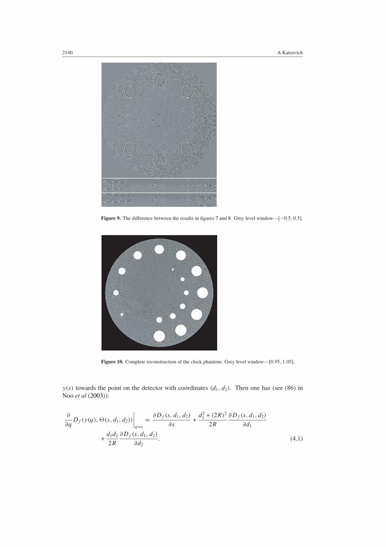
Figure 9. The difference between the results in figures 7 and 8. Grey level window—[−0.5, 0.5].

Figure 10. Complete reconstruction of the clock phantom. Grey level window—[0.95, 1.05].

y(s) towards the point on the detector with coordinates (d1, d2). Then one has (see (86) inNoo et al (2003)):

∂

∂qDf (y(q),�(s, d1, d2))

∣∣∣∣q=s

= ∂Df (s, d1, d2)

∂s+

d21 + (2R)2

2R

∂Df (s, d1, d2)

∂d1

+d1d2

2R

∂Df (s, d1, d2)

∂d2. (4.1)

On two versions of a 3π algorithm for spiral CT 2141

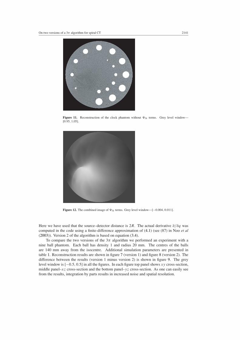
Figure 11. Reconstruction of the clock phantom without �3k terms. Grey level window—[0.95, 1.05].

Figure 12. The combined image of �3k terms. Grey level window—[−0.004, 0.011].

Here we have used that the source–detector distance is 2R. The actual derivative ∂/∂q wascomputed in the code using a finite-difference approximation of (4.1) (see (87) in Noo et al(2003)). Version 2 of the algorithm is based on equation (3.4).

To compare the two versions of the 3π algorithm we performed an experiment with anine ball phantom. Each ball has density 1 and radius 20 mm. The centres of the ballsare 140 mm away from the isocentre. Additional simulation parameters are presented intable 1. Reconstruction results are shown in figure 7 (version 1) and figure 8 (version 2). Thedifference between the results (version 1 minus version 2) is shown in figure 9. The greylevel window is [−0.5, 0.5] in all the figures. In each figure top panel shows xy cross-section,middle panel–xz cross-section and the bottom panel–yz cross-section. As one can easily seefrom the results, integration by parts results in increased noise and spatial resolution.

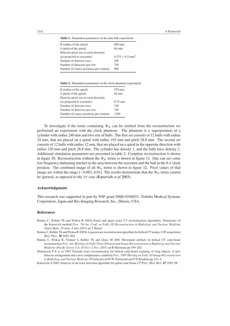
2142 A Katsevich

Table 1. Simulation parameters in the nine ball experiment.

R (radius of the spiral) 600 mmh (pitch of the spiral) 66 mmDetector pixel size in each direction(as projected to isocentre) 0.575 × 0.5 mm2

Number of detector rows 256Number of detectors per row 750Number of source positions per rotation 900

Table 2. Simulation parameters in the clock phantom experiment.

R (radius of the spiral) 570 mmh (pitch of the spiral) 46 mmDetector pixel size in each direction(as projected to isocentre) 0.75 mmNumber of detector rows 128Number of detectors per row 745Number of source positions per rotation 1160

To investigate if the terms containing �3k can be omitted from the reconstruction weperformed an experiment with the clock phantom. The phantom is a superposition of acylinder with radius 240 mm and two sets of balls. The first set consists of 12 balls with radius24 mm, that are placed on a spiral with radius 192 mm and pitch 28.8 mm. The second setconsists of 12 balls with radius 12 mm, that are placed on a spiral in the opposite direction withradius 120 mm and pitch 28.8 mm. The cylinder has density 1, and the balls have density 2.Additional simulation parameters are presented in table 2. Complete reconstruction is shownin figure 10. Reconstruction without the �3k terms is shown in figure 11. One can see somelow frequency darkening artefact in the area between the isocentre and the ball in the 8 o’clockposition. The combined image of all �3k terms is shown in figure 12. Pixel values of thatimage are within the range [−0.003, 0.01]. The results demonstrate that the �3k terms cannotbe ignored, as opposed to the 1π case (Katsevich et al 2003).

Acknowledgments

This research was supported in part by NSF grant DMS-0104033, Toshiba Medical SystemsCorporation, Japan and Bio-Imaging Research, Inc., Illinois, USA.

References

Bontus C, Kohler Th and Proksa R 2003a Exact and quasi exact CT reconstruction algorithms. Extensions ofthe Katsevich method Proc. 7th Int. Conf. on Fully 3D Reconstruction in Radiology and Nuclear Medicine(Saint-Malo, 29 June–4 July 2003) ed Y Bizais

Bontus C, Kohler Th and Proksa R 2003b A quasiexact reconstruction algorithm for helical CT using a 3-PI acquisitionMed. Phys. 30 2493–502

Bontus C, Proksa R, Timmer J, Kohler Th and Grass M 2001 Movement artifacts in helical CT cone-beamreconstruction Proc. Int. Meeting on Fully Three-Dimensional Image Reconstruction in Radiology and NuclearMedicine (Pacific Grove, CA, 30 Oct.–2 Nov. 2001) ed R Huesman pp 199–202

Danielsson P E et al 1997 Towards exact reconstruction for helical cone-beam scanning of long objects. A newdetector arrangement and a new completeness condition Proc. 1997 Meeting on Fully 3D Image Reconstructionin Radiology and Nuclear Medicine (Pittsburgh) ed D W Townsend and P E Kinahan pp 141–4

Katsevich A 2002 Analysis of an exact inversion algorithm for spiral cone-beam CT Phys. Med. Biol. 47 2583–98

On two versions of a 3π algorithm for spiral CT 2143

Katsevich A 2003 A generalized inversion formula for cone beam CT Proc. 7th Int. Conf. on Fully 3D Reconstructionin Radiology and Nuclear Medicine (Saint-Malo 29 June–4 July 2003) ed Y Bizais

Katsevich A 2004 3π algorithm for spiral CT (submitted)Katsevich A, Lauritsch G, Bruder H, Flohr T and Stierstorfer K 2003 Evaluation and empirical analysis of an

exact FBP algorithm for spiral cone-beam CT Proc. SPIE 2003 Medical Imaging Conference ed M Sonka andJ M Fitzpatrick Proc. SPIE 5032 663–74

Kohler Th, Proksa R, Bontus C, Grass M and Timmer J 2002 Artifact analysis of approximate cone-beam CTalgorithms Med. Phys. 29 51–64

Noo F, Pack J and Heuscher D 2003 Exact helical reconstruction using native cone-beam geometries Phys. Med. Biol.48 3787–818

Proksa R, Kohler Th, Grass M and Timmer J 2000 The n-PI method for helical conebeam CT IEEE Trans. Med.Imaging 19 848–63

Tam K C 1995 Three-dimensional computerized tomography scanning method and system for imaging large objectswith smaller area detectors US Patent 5,390,112

Tam K C, Samarasekera S and Sauer F 1998 Exact cone beam CT with a spiral scan Phys. Med. Biol. 43 1015–24