JJ311 MECHANICAL OF MACHINE Ch 3 Velocity and Acceleration Diagram
Numerical Optimization using the Levenberg-Marquardt Algorithm
Leif Zinn-Bjorkman
EES-16
LA-UR-11-12010
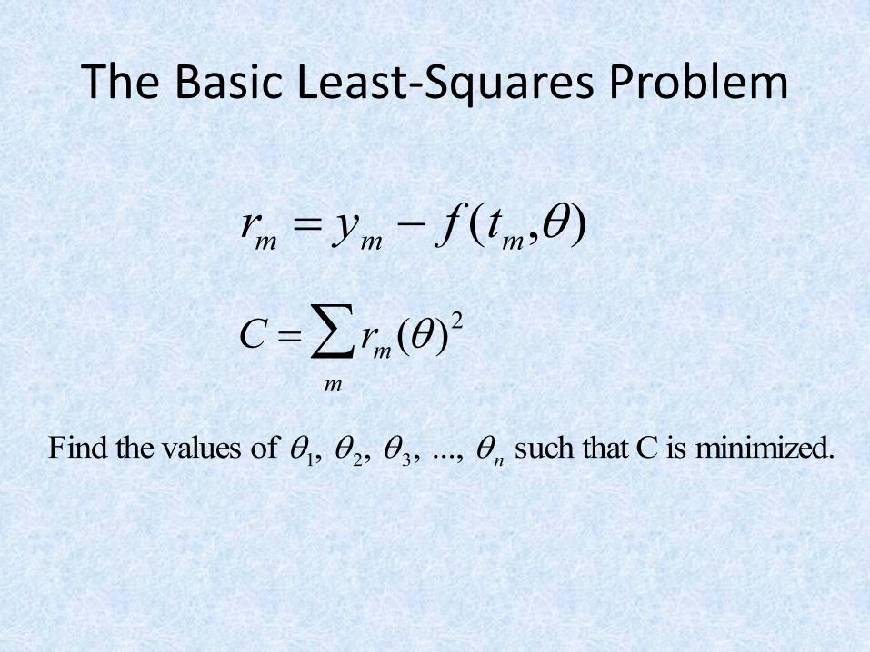
The Basic Least-Squares Problem
rm ym f (tm,)
C rm ()2
m
Find the values of 1, 2, 3, ..., n such that C is minimized.
Optimization Algorithms
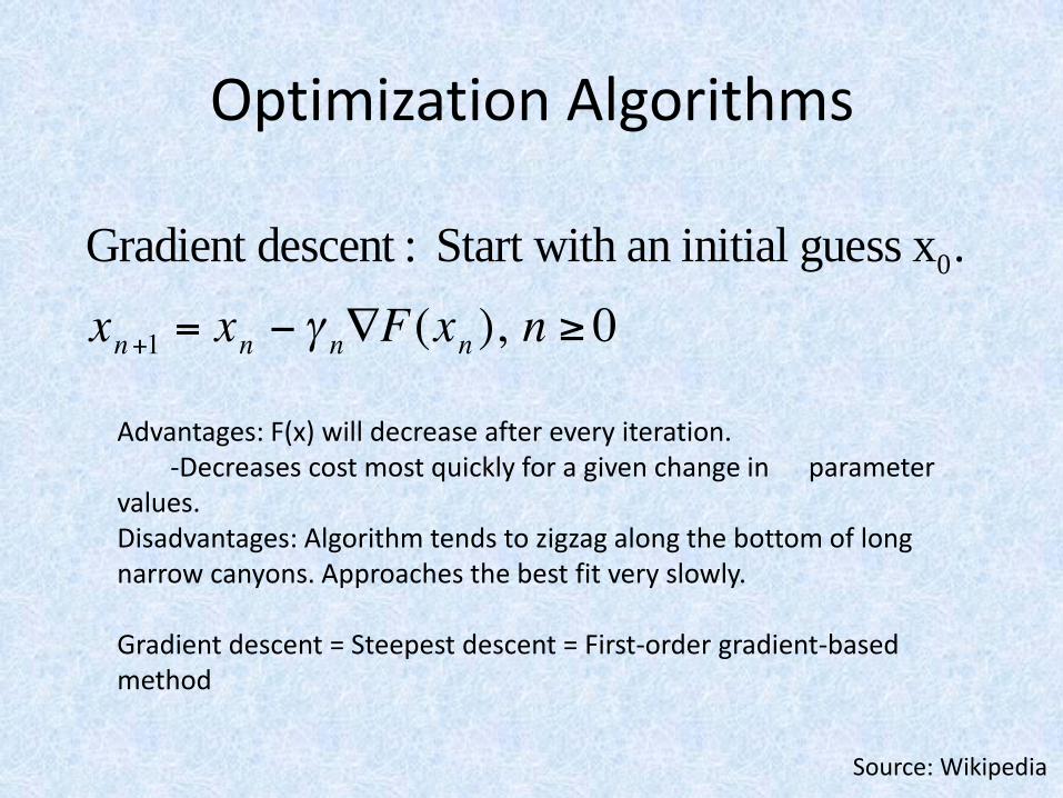
Gradient descent : Start with an initial guess x0.
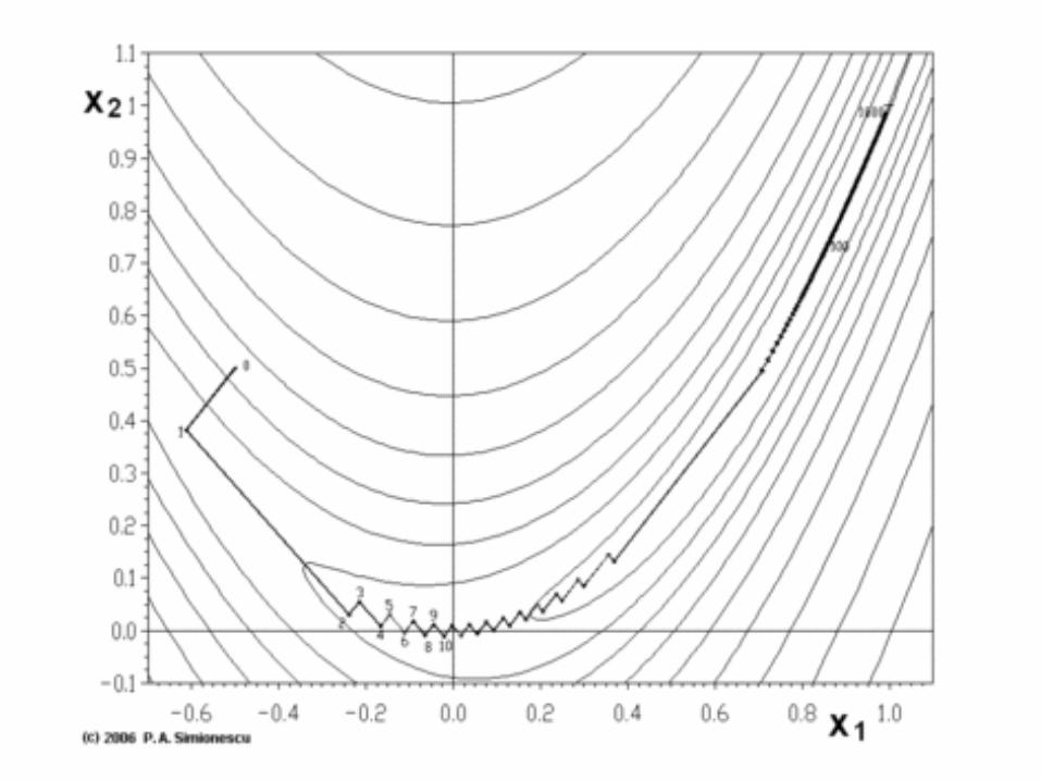
Advantages: F(x) will decrease after every iteration. -Decreases cost most quickly for a given change in parameter values. Disadvantages: Algorithm tends to zigzag along the bottom of long narrow canyons. Approaches the best fit very slowly. Gradient descent = Steepest descent = First-order gradient-based method
Source: Wikipedia
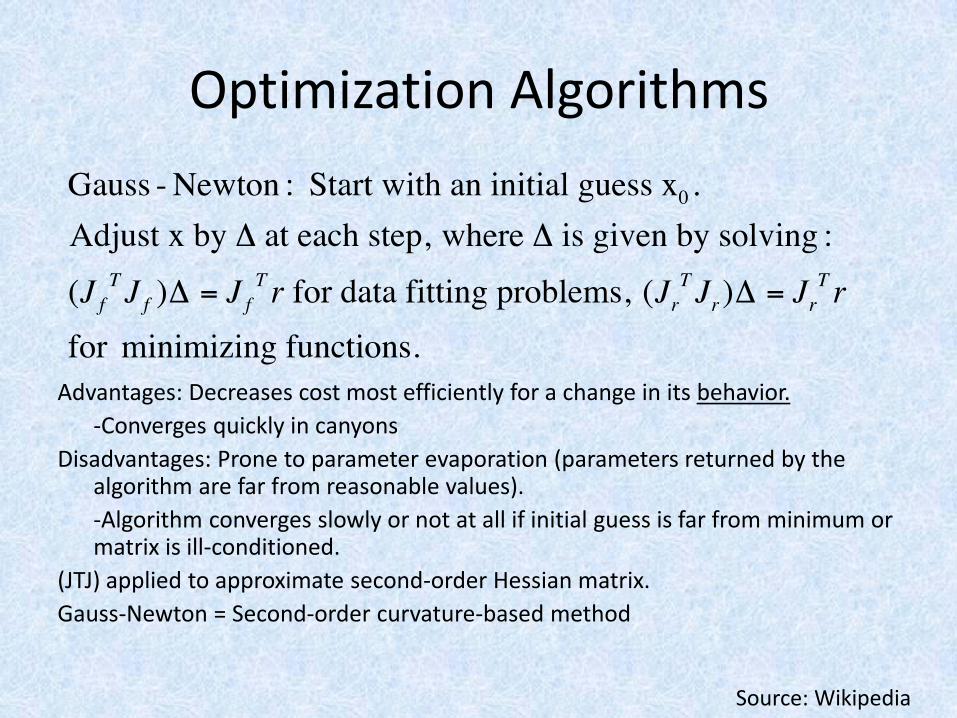
Optimization Algorithms
Advantages: Decreases cost most efficiently for a change in its behavior.
-Converges quickly in canyons
Disadvantages: Prone to parameter evaporation (parameters returned by the algorithm are far from reasonable values).
-Algorithm converges slowly or not at all if initial guess is far from minimum or matrix is ill-conditioned.
(JTJ) applied to approximate second-order Hessian matrix.
Gauss-Newton = Second-order curvature-based method
Source: Wikipedia
The Levenberg-Marquardt Algorithm
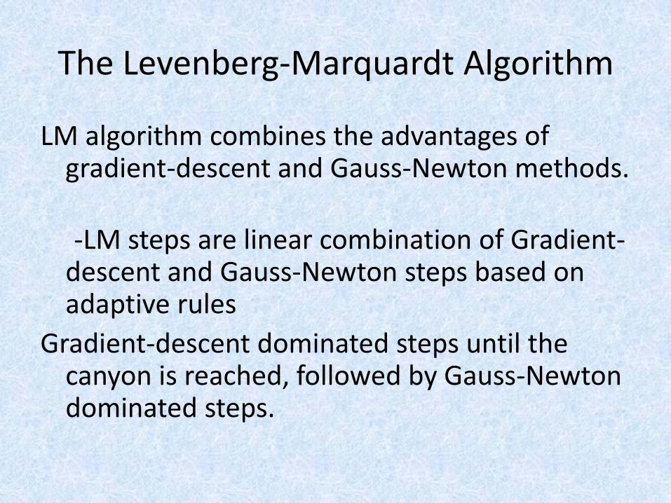
LM algorithm combines the advantages of gradient-descent and Gauss-Newton methods.
-LM steps are linear combination of Gradient-descent and Gauss-Newton steps based on adaptive rules
Gradient-descent dominated steps until the canyon is reached, followed by Gauss-Newton dominated steps.
The Levenberg-Marquardt Algorithm
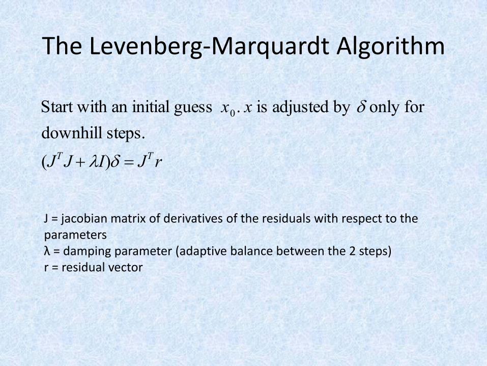
J = jacobian matrix of derivatives of the residuals with respect to the parameters λ = damping parameter (adaptive balance between the 2 steps) r = residual vector
Start with an initial guess x0. x is adjusted by only for
downhill steps.
(JTJ I) JT r
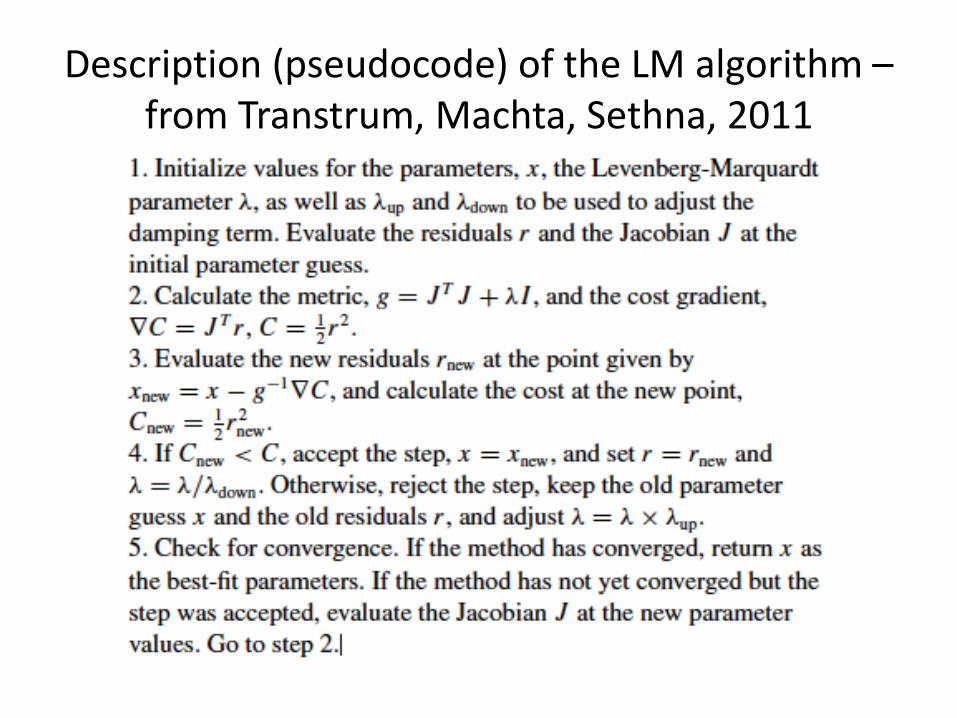
Description (pseudocode) of the LM algorithm – from Transtrum, Machta, Sethna, 2011
LevMar Convergence Criteria as implemented in MADS
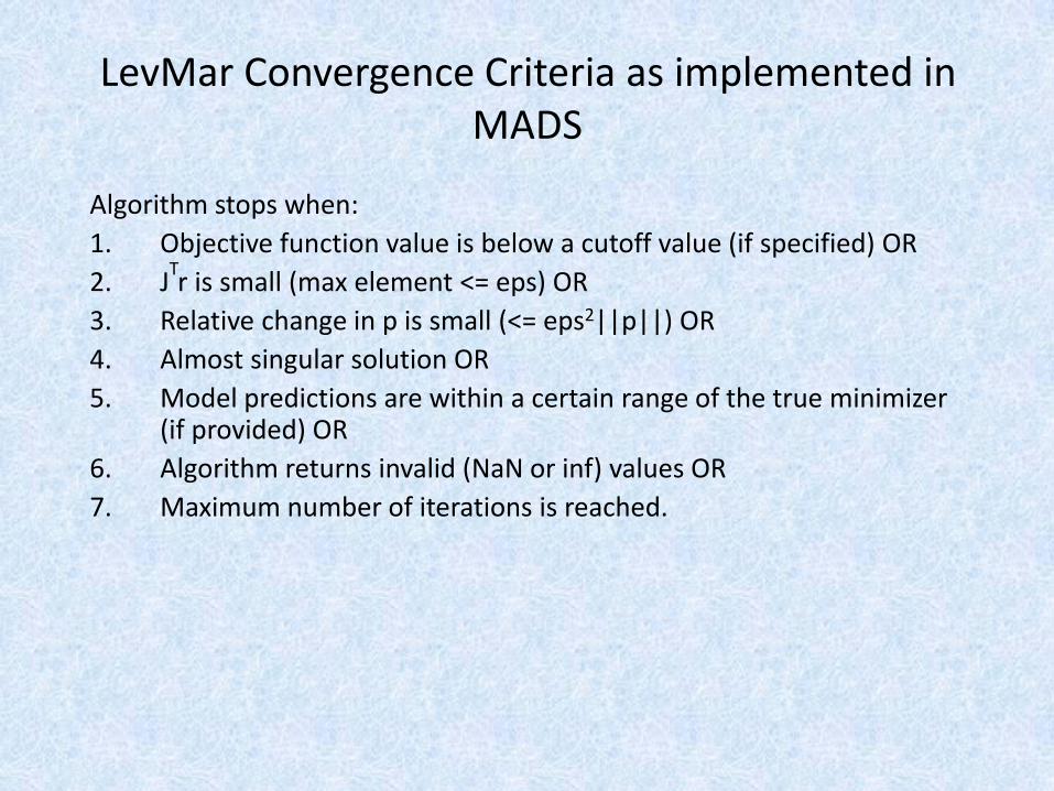
Algorithm stops when:
1. Objective function value is below a cutoff value (if specified) OR
2. JTr is small (max element <= eps) OR
3. Relative change in p is small (<= eps2||p||) OR
4. Almost singular solution OR
5. Model predictions are within a certain range of the true minimizer (if provided) OR
6. Algorithm returns invalid (NaN or inf) values OR
7. Maximum number of iterations is reached.
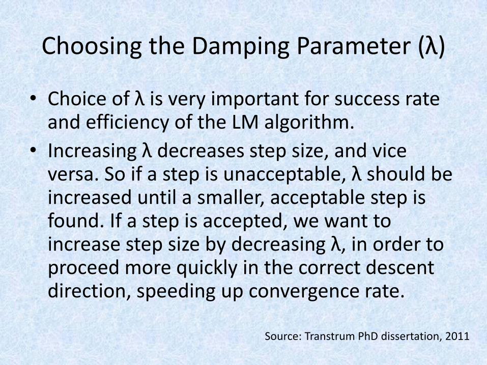
Choosing the Damping Parameter (λ)
• Choice of λ is very important for success rate and efficiency of the LM algorithm.
• Increasing λ decreases step size, and vice versa. So if a step is unacceptable, λ should be increased until a smaller, acceptable step is found. If a step is accepted, we want to increase step size by decreasing λ, in order to proceed more quickly in the correct descent direction, speeding up convergence rate.
Source: Transtrum PhD dissertation, 2011
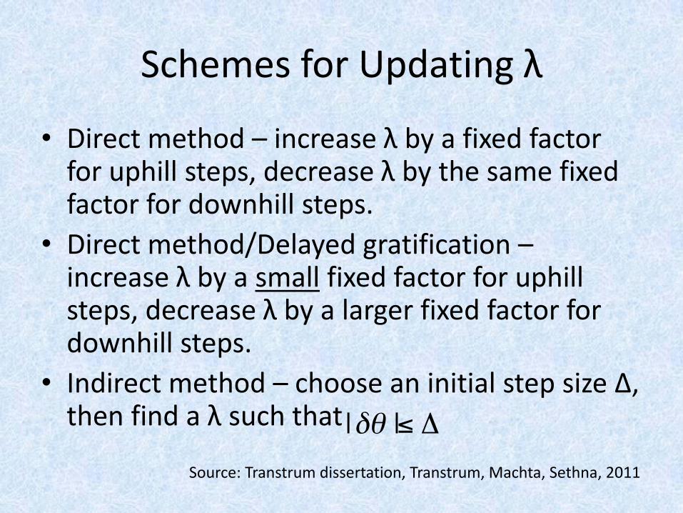
Schemes for Updating λ
• Direct method – increase λ by a fixed factor for uphill steps, decrease λ by the same fixed factor for downhill steps.
• Direct method/Delayed gratification – increase λ by a small fixed factor for uphill steps, decrease λ by a larger fixed factor for downhill steps.
• Indirect method – choose an initial step size Δ, then find a λ such that
Source: Transtrum dissertation, Transtrum, Machta, Sethna, 2011
Motivation for Delayed Gratification Method
• Direct method with equal up and down adjustments tends to move downhill too quickly, greatly reducing steps that will be allowed at successive iterations, which slows convergence rate (although it appears to have no effect on success rate).
• By using delayed gratification, we choose the smallest λ that does not produce an uphill step, which slows initial downhill progression but speeds up convergence rate near the solution.
Source: Transtrum, Machta, Sethna, 2011
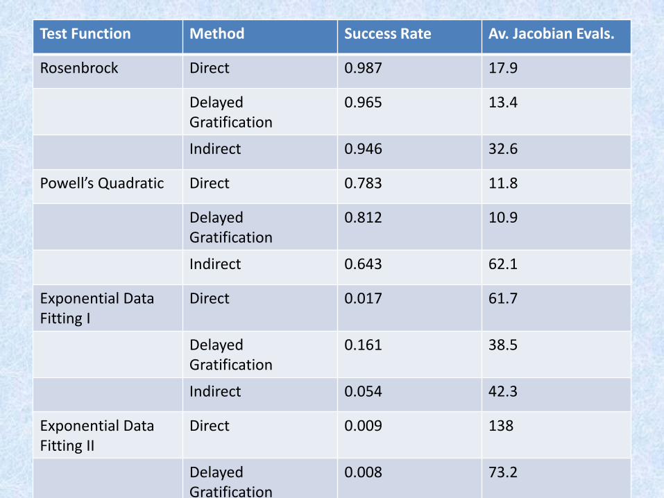
Test Function Method Success Rate Av. Jacobian Evals.
Rosenbrock Direct 0.987 17.9
Delayed Gratification
0.965 13.4
Indirect 0.946 32.6
Powell’s Quadratic Direct 0.783 11.8
Delayed Gratification
0.812 10.9
Indirect 0.643 62.1
Exponential Data Fitting I
Direct 0.017 61.7
Delayed Gratification
0.161 38.5
Indirect 0.054 42.3
Exponential Data Fitting II
Direct 0.009 138
Delayed Gratification
0.008 73.2
Indirect 0.013 167
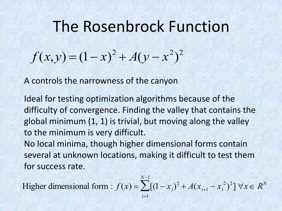
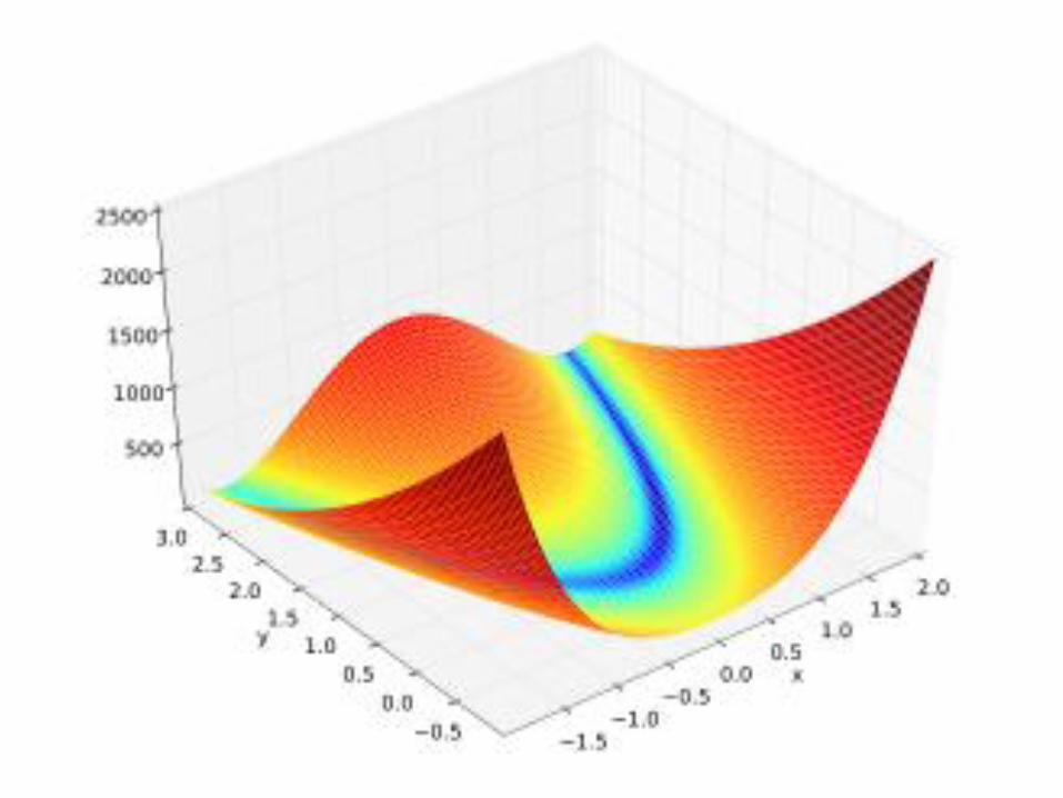
The Rosenbrock Function
Ideal for testing optimization algorithms because of the difficulty of convergence. Finding the valley that contains the global minimum (1, 1) is trivial, but moving along the valley to the minimum is very difficult. No local minima, though higher dimensional forms contain several at unknown locations, making it difficult to test them for success rate.
A controls the narrowness of the canyon
f (x,y) (1 x)2 A(y x2)2
Higher dimensional form : f (x) [(1 xi)2 A(xi1 xi
2)2]
i1
N 1
xRN
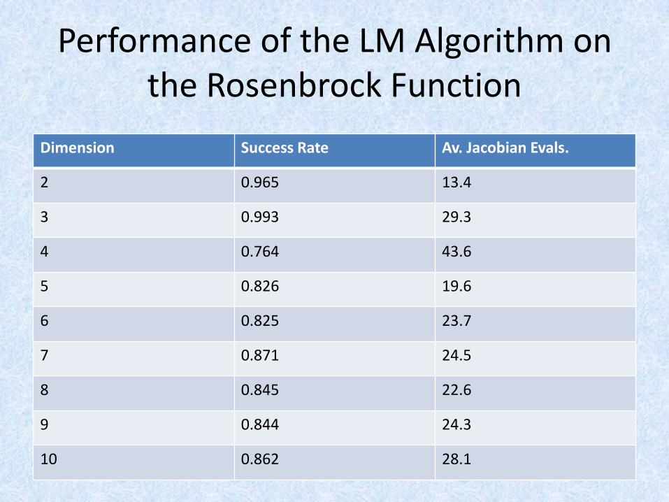
Performance of the LM Algorithm on the Rosenbrock Function
Dimension Success Rate Av. Jacobian Evals.
2 0.965 13.4
3 0.993 29.3
4 0.764 43.6
5 0.826 19.6
6 0.825 23.7
7 0.871 24.5
8 0.845 22.6
9 0.844 24.3
10 0.862 28.1
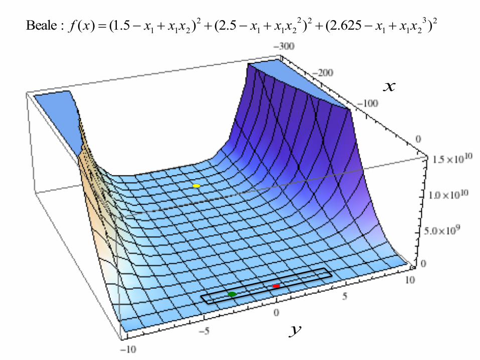
Beale : f (x) (1.5 x1 x1x2)2 (2.5 x1 x1x2
2)2 (2.625 x1 x1x2
3)2
x
y
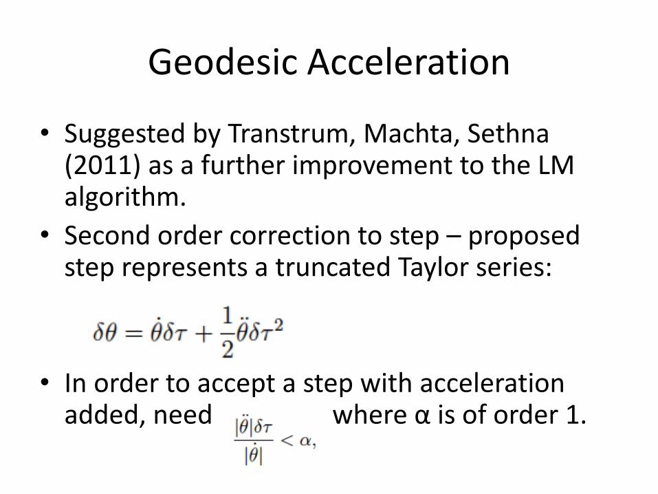
Geodesic Acceleration
• Suggested by Transtrum, Machta, Sethna (2011) as a further improvement to the LM algorithm.
• Second order correction to step – proposed step represents a truncated Taylor series:
• In order to accept a step with acceleration added, need where α is of order 1.
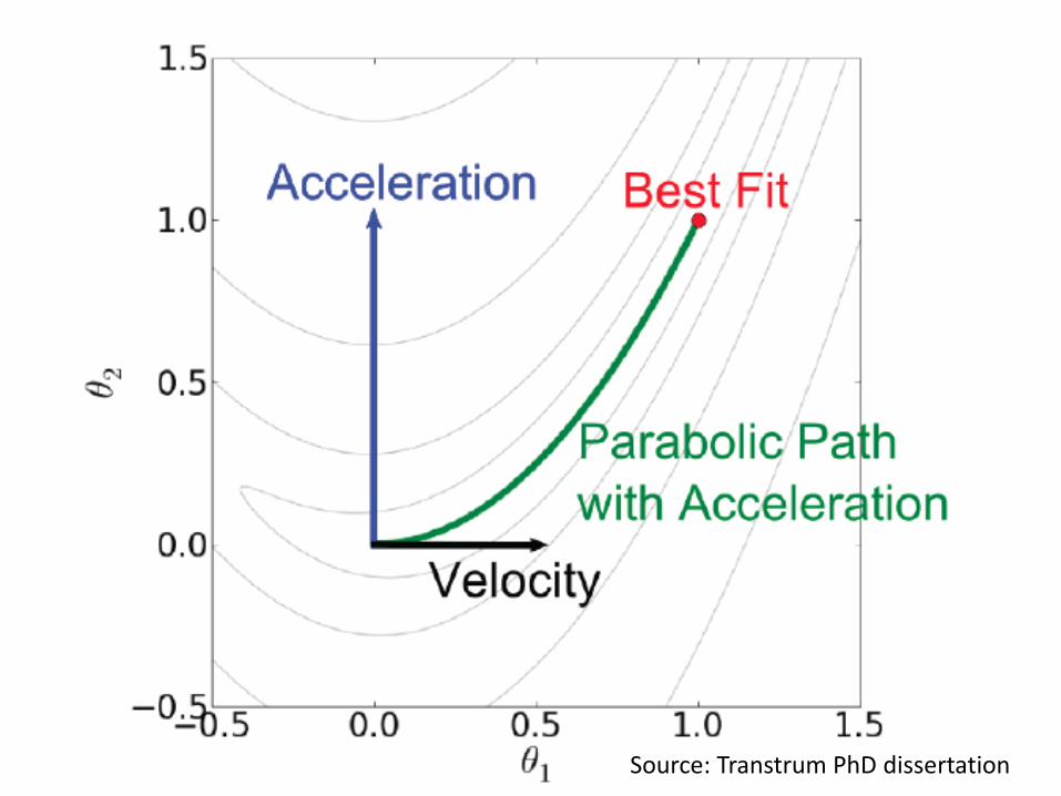
Source: Transtrum PhD dissertation
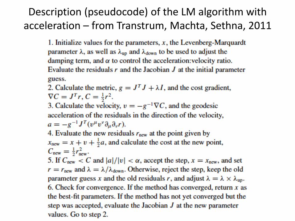
Description (pseudocode) of the LM algorithm with acceleration – from Transtrum, Machta, Sethna, 2011
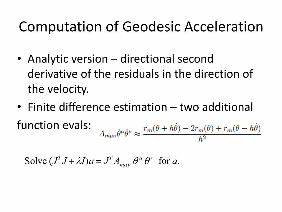
Computation of Geodesic Acceleration
• Analytic version – directional second derivative of the residuals in the direction of the velocity.
• Finite difference estimation – two additional
function evals:
Solve (JTJ I)a JTAm for a.
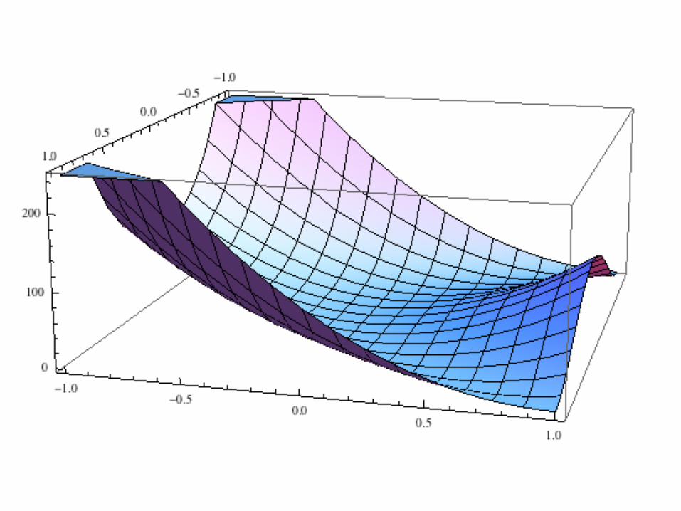
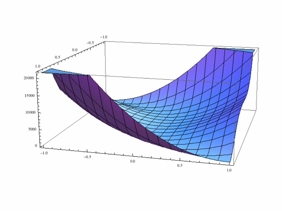
Modified Rosenbrock Function
• Used to demonstrate effectiveness of adding acceleration to algorithm.
• Residuals given by:
A and n control narrowness of the canyon – as A and n increase, canyon narrows. Global minimum at (0,0).
x, A(y xn ) (n 2)
Function : f (x,y) x2 A2(y xn )2
Modified Rosenbrock Tests
• Tested function with 4 different “complexities”:
1. A = 10, n = 2
2. A = 100, n = 3
3. A = 1000, n = 4
4. A = 1000, n = 5
Initial Guess: (1,1) Convergence criteria: OF < 1e-12
• Comparison between non-acceleration and acceleration versions of algorithm (both with delayed gratification technique for updating λ).
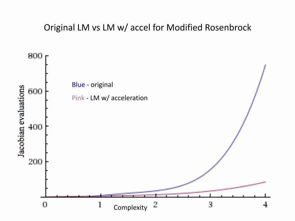
Original LM vs LM w/ accel for Modified Rosenbrock
Blue - original
Pink - LM w/ acceleration
Complexity
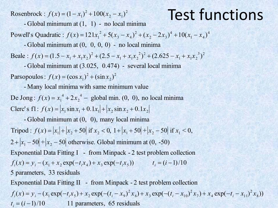
Test functions
Rosenbrock : f (x) (1 x1)2 100(x2 x1)
2
- Global minimum at (1, 1) - no local minima
Powell's Quadratic : f (x) 121x1
2 5(x3 x4 )2 (x2 2x3)4 10(x1 x4 )4
- Global minimum at (0, 0, 0, 0) - no local minima
Beale : f (x) (1.5 x1 x1x2)2 (2.5 x1 x1x2
2)2 (2.625 x1 x1x2
3)2
- Global minimum at (3.025, 0.474) - several local minima
Parsopoulos : f (x) (cos x1)2 (sin x2)2
- Many local minima with same minimum value
De Jong : f (x) x1
4 2x2
4 global min. (0, 0), no local minima
Clerc' s f1: f (x) x1 sin x1 0.1x1 x2 sin x2 0.1x2
- Global minimum at (0, 0), many local minima
Tripod : f (x) x1 x2 50 if x2 0, 1 x1 50 + x2 50 if x1 < 0,
2 x1 50 + x2 50 otherwise. Global minimum at (0, -50)
Exponential Data Fitting I - from Minpack - 2 test problem collection
f i(x) y i (x1 x2 exp(tix4 ) x3 exp(tix5)) ti (i 1) /10
5 parameters, 33 residuals
Exponential Data Fitting II - from Minpack - 2 test problem collection
f i(x) y i (x1 exp(tix5) x2 exp((ti x9)2 x 6) x3 exp((ti x10)2 x7) x4 exp(ti x11)
2 x8))
ti (i 1) /10 11 parameters, 65 residuals
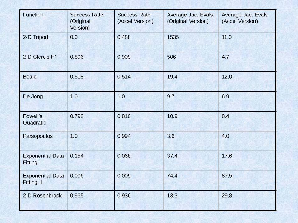
Function Success Rate
(Original
Version)
Success Rate
(Accel Version)
Average Jac. Evals.
(Original Version)
Average Jac. Evals
(Accel Version)
2-D Tripod 0.0 0.488 1535 11.0
2-D Clerc’s F1 0.896 0.909 506 4.7
Beale 0.518 0.514 19.4 12.0
De Jong 1.0 1.0 9.7 6.9
Powell’s
Quadratic
0.792 0.810 10.9 8.4
Parsopoulos 1.0 0.994 3.6 4.0
Exponential Data
Fitting I
0.154 0.068 37.4 17.6
Exponential Data
Fitting II
0.006 0.009 74.4 87.5
2-D Rosenbrock 0.965 0.936 13.3 29.8
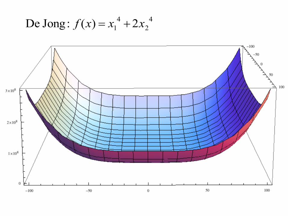
De Jong: f (x) x1
42x2
4
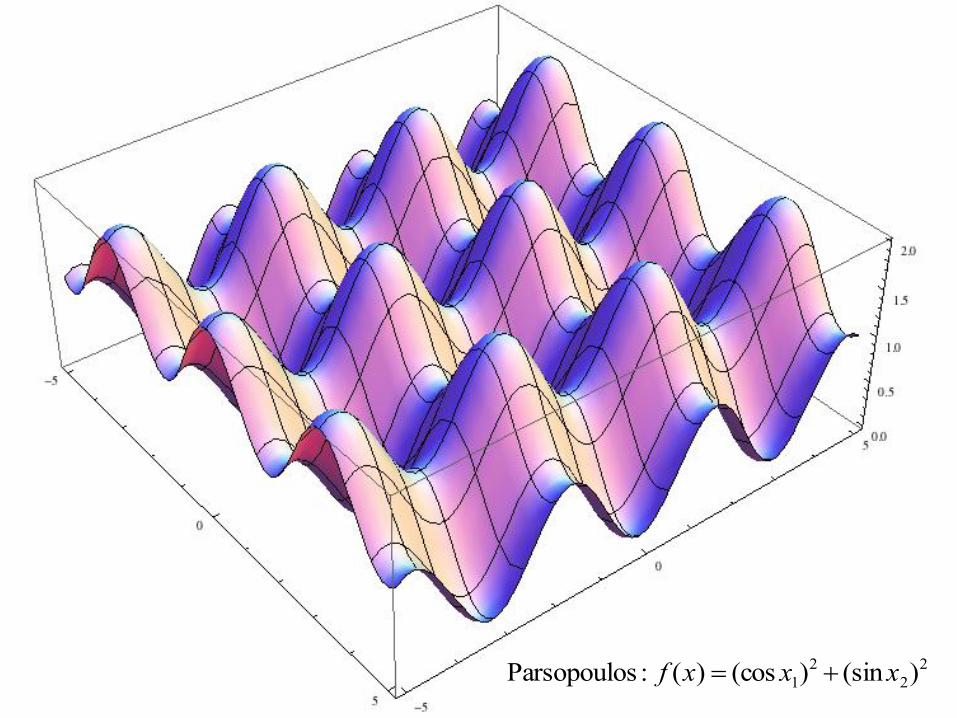
Parsopoulos : f (x) (cos x1)2 (sinx2)
2
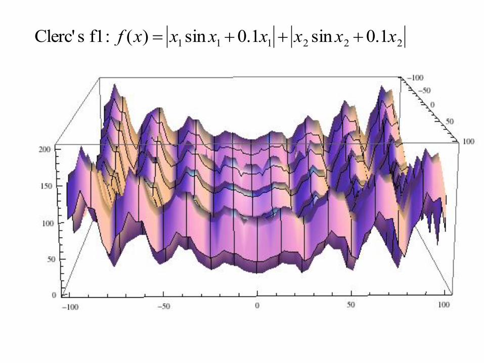
Clerc' s f1: f (x) x1 sinx1 0.1x1 x2 sin x2 0.1x2
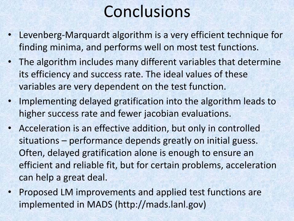
Conclusions • Levenberg-Marquardt algorithm is a very efficient technique for
finding minima, and performs well on most test functions.
• The algorithm includes many different variables that determine its efficiency and success rate. The ideal values of these variables are very dependent on the test function.
• Implementing delayed gratification into the algorithm leads to higher success rate and fewer jacobian evaluations.
• Acceleration is an effective addition, but only in controlled situations – performance depends greatly on initial guess. Often, delayed gratification alone is enough to ensure an efficient and reliable fit, but for certain problems, acceleration can help a great deal.
• Proposed LM improvements and applied test functions are implemented in MADS (http://mads.lanl.gov)