Lecture 3

C7B Optimization Hilary 2011 A. Zisserman

Cost functions with special structure:

• Levenberg-Marquardt algorithm

• Dynamic Programming• chains

• applications

First: review Gauss-Newton approximation

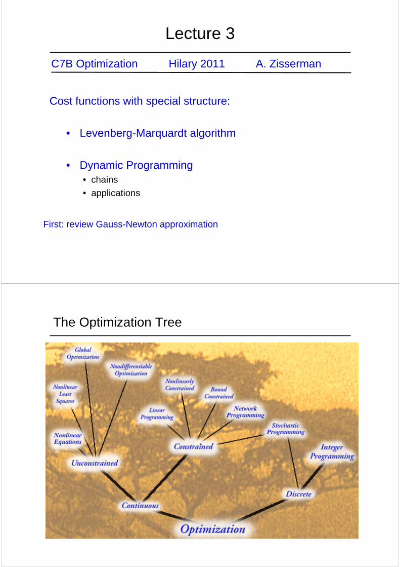
The Optimization Tree

Summary of minimizations methods

Update xn+1 = xn+ δx

1. Newton.

H δx = −g

2. Gauss-Newton.

2J>J δx = −g

3. Gradient descent.

λδx = −g

Levenberg-Marquardt algorithm

-1 -0.8 -0.6 -0.4 -0.2 0 0.2 0.4 0.6 0.8 10

0.2

0.4

0.6

0.8

1

1.2

1.4

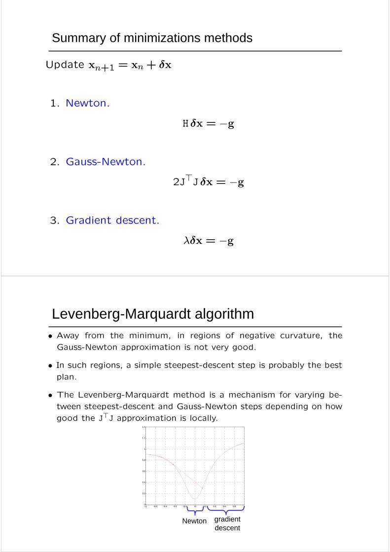
• Away from the minimum, in regions of negative curvature, the

Gauss-Newton approximation is not very good.

• In such regions, a simple steepest-descent step is probably the bestplan.

• The Levenberg-Marquardt method is a mechanism for varying be-

tween steepest-descent and Gauss-Newton steps depending on how

good the J>J approximation is locally.

gradient descent

Newton

• The method uses the modified Hessian

H (x,λ) = 2J>J+ λI

• When λ is small, H approximates the Gauss-Newton Hessian.

• When λ is large, H is close to the identity, causing steepest-descent

steps to be taken.

LM Algorithm

H (x,λ) = 2J>J+ λI

1. Set λ = 0.001 (say)

2. Solve δx = −H(x,λ)−1 g

3. If f(xn+ δx) > f(xn), increase λ (×10 say) and go to 2.

4. Otherwise, decrease λ (×0.1 say), let xn+1 = xn+ δx, and go to 2.

Note : This algorithm does not require explicit line searches.

Example

-2 -1.5 -1 -0.5 0 0.5 1 1.5 2-1

-0.5

0

0.5

1

1.5

2

2.5

3Levenberg-Marquardt method

gradient < 1e-3 after 31 iterations-2 -1 0 1 2

-1

-0.5

0

0.5

1

1.5

2

2.5

3Levenberg-Marquardt method

gradient < 1e-3 after 31 iterations

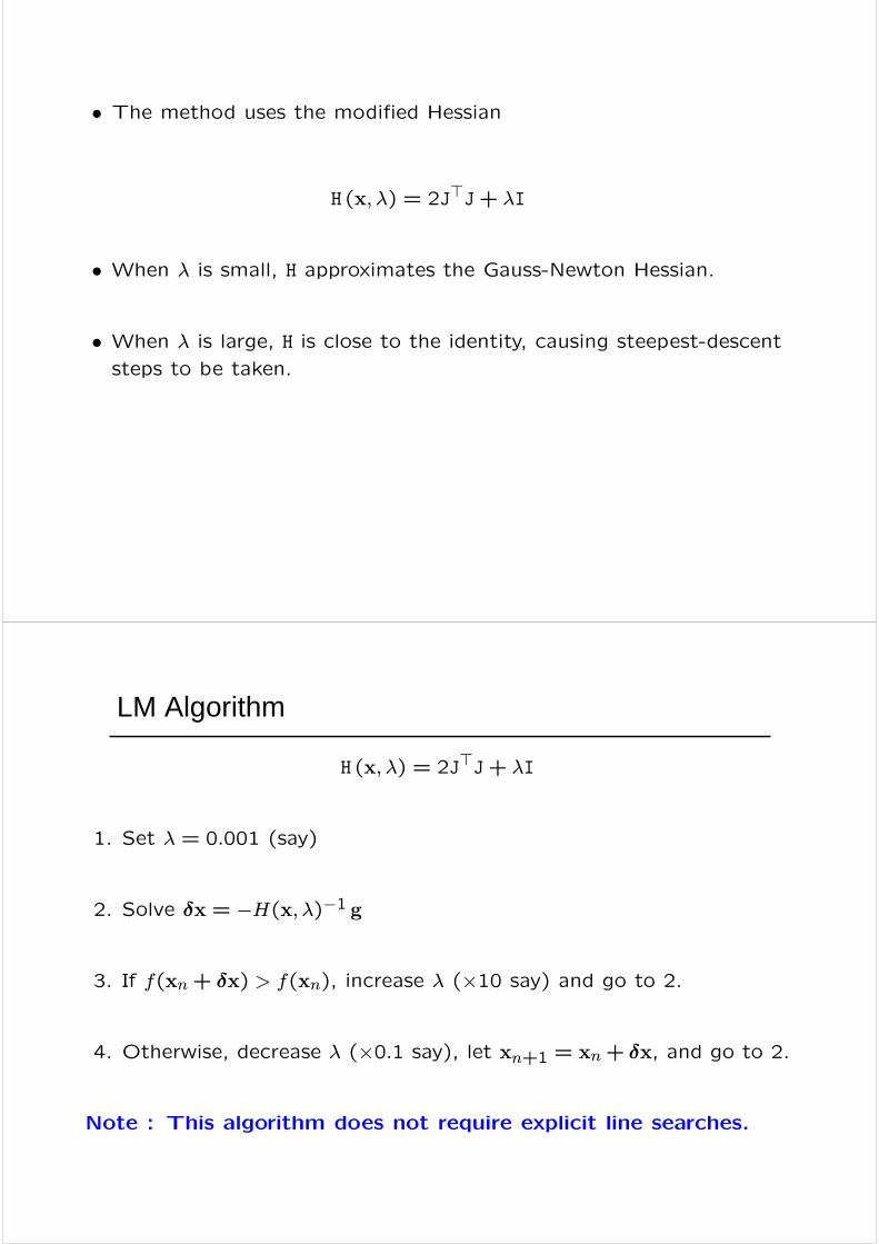
• Minimization using Levenberg-Marquardt (no line search) takes 31iterations.

Matlab: lsqnonlin

Comparison

-2 -1 0 1 2-1

-0.5

0

0.5

1

1.5

2

2.5

3Levenberg-Marquardt method

gradient < 1e-3 after 31 iterations

-2 -1 0 1 2-1

-0.5

0

0.5

1

1.5

2

2.5

3Gauss-Newton method with line search

gradient < 1e-3 after 14 iterations

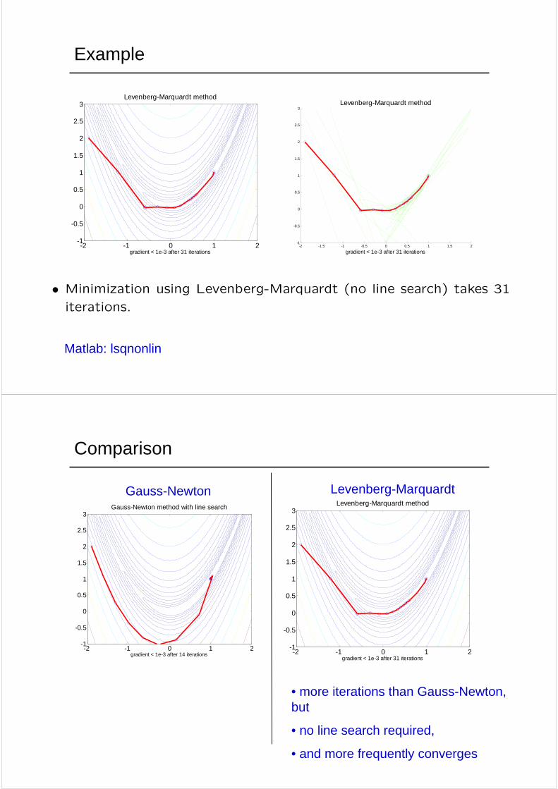
Gauss-Newton

• more iterations than Gauss-Newton, but

• no line search required,

• and more frequently converges

Levenberg-Marquardt

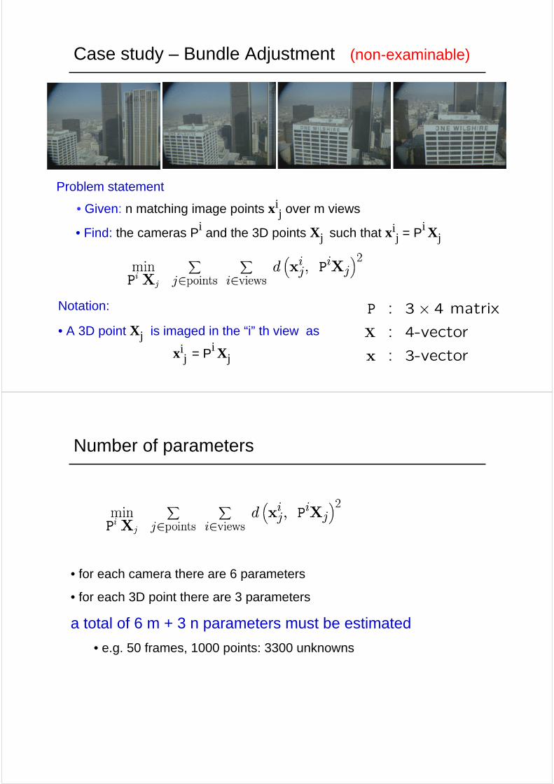
Case study – Bundle Adjustment (non-examinable)

Notation:

• A 3D point Xj is imaged in the “i” th view as

xij = Pi Xj

P : 3× 4 matrixX : 4-vector

x : 3-vector

Problem statement

• Given: n matching image points xij over m views

• Find: the cameras Pi and the 3D points Xj such that xij = Pi Xj

Number of parameters

• for each camera there are 6 parameters

• for each 3D point there are 3 parameters

a total of 6 m + 3 n parameters must be estimated

• e.g. 50 frames, 1000 points: 3300 unknowns

Example

image sequence cameras and points

Sparse form of the Jacobian matrix

• Image point xij does not depend on the parameters of any cameraother than Pi.

• Thus,∂xij/∂P

k = 0

unless i = k.

• Similarly, image point xij does not depend on any 3D point except

Xj.

∂xij/∂Xk = 0

unless j = k.

Form of the Jacobian and Gauss-Newton Hessian for the bundle-adjustment problem consisting of 3 cameras and 4 points.

J>JJ

By taking advantage of this sparse form, one iterative update of the

LM algorithm

• H (x,λ) = 2J>J+ λI

• Solve δx = −H(x,λ)−1 g

can be solved in O(N) rather than O(N3), where N is the total number

of parameters

= 0

Application: Augmented reality

original sequence

Augmentation

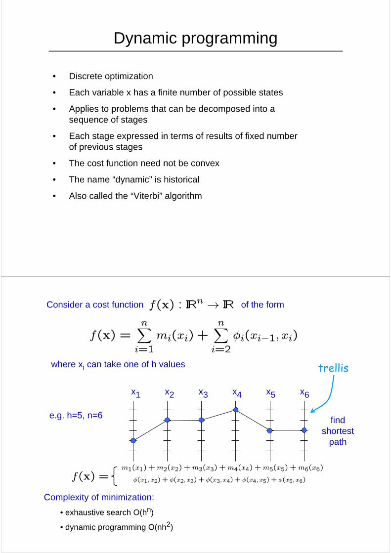
Dynamic programming

• Discrete optimization

• Each variable x has a finite number of possible states

• Applies to problems that can be decomposed into a sequence of stages

• Each stage expressed in terms of results of fixed number of previous stages

• The cost function need not be convex

• The name “dynamic” is historical

• Also called the “Viterbi” algorithm

Consider a cost function of the form

where xi can take one of h values

e.g. h=5, n=6

x1 x2 x3 x4 x5 x6

f(x) : IRn → IR

f(x) =

find shortest

path

Complexity of minimization:

• exhaustive search O(hn)

• dynamic programming O(nh2)

f(x) =nXi=1

mi(xi) +nXi=2

φi(xi−1, xi)

m1(x1) +m2(x2) +m3(x3) +m4(x4) +m5(x5) +m6(x6)

φ(x1, x2) + φ(x2, x3) + φ(x3, x4) + φ(x4, x5) + φ(x5, x6)

trellis

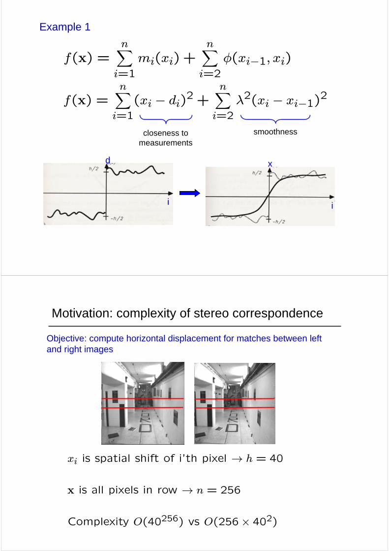
Example 1

closeness to measurements

smoothness

f(x) =nXi=1

(xi − di)2 +nXi=2

λ2(xi − xi−1)2

f(x) =nXi=1

mi(xi) +nXi=2

φ(xi−1, xi)

d

i

x

i

Motivation: complexity of stereo correspondence

Objective: compute horizontal displacement for matches between left and right images

xi is spatial shift of i’th pixel → h = 40

x is all pixels in row → n = 256

Complexity O(40256) vs O(256× 402)

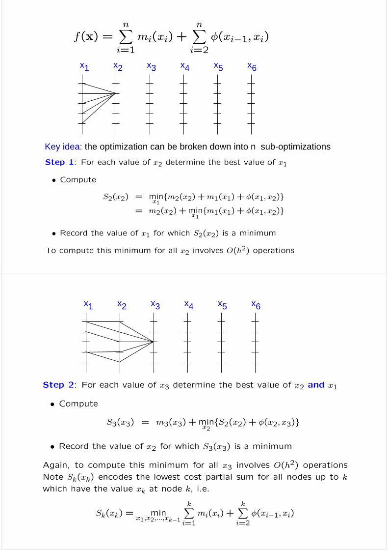
x1 x2 x3 x4 x5 x6

Key idea: the optimization can be broken down into n sub-optimizations

f(x) =nXi=1

mi(xi) +nXi=2

φ(xi−1, xi)

Step 1: For each value of x2 determine the best value of x1

• Compute

S2(x2) = minx1{m2(x2) +m1(x1) + φ(x1, x2)}

= m2(x2) +minx1{m1(x1) + φ(x1, x2)}

• Record the value of x1 for which S2(x2) is a minimum

To compute this minimum for all x2 involves O(h2) operations

x1 x2 x3 x4 x5 x6

Step 2: For each value of x3 determine the best value of x2 and x1

• Compute

S3(x3) = m3(x3) +minx2{S2(x2) + φ(x2, x3)}

• Record the value of x2 for which S3(x3) is a minimum

Again, to compute this minimum for all x3 involves O(h2) operations

Note Sk(xk) encodes the lowest cost partial sum for all nodes up to k

which have the value xk at node k, i.e.

Sk(xk) = minx1,x2,...,xk−1

kXi=1

mi(xi) +kXi=2

φ(xi−1, xi)

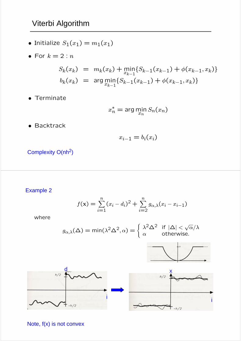
Viterbi Algorithm

Complexity O(nh2)

• Initialize S1(x1) = m1(x1)

• For k = 2 : n

Sk(xk) = mk(xk) + minxk−1

{Sk−1(xk−1) + φ(xk−1, xk)}bk(xk) = argmin

xk−1{Sk−1(xk−1) + φ(xk−1, xk)}

• Terminatex∗n = argmin

xnSn(xn)

• Backtrackxi−1 = bi(xi)

Example 2

Note, f(x) is not convex

f(x) =nXi=1

(xi − di)2 +nXi=2

gα,λ(xi − xi−1)

where

gα,λ(∆) = min(λ2∆2,α) =

(λ2∆2 if |∆| < √α/λα otherwise.

i

d

i

x

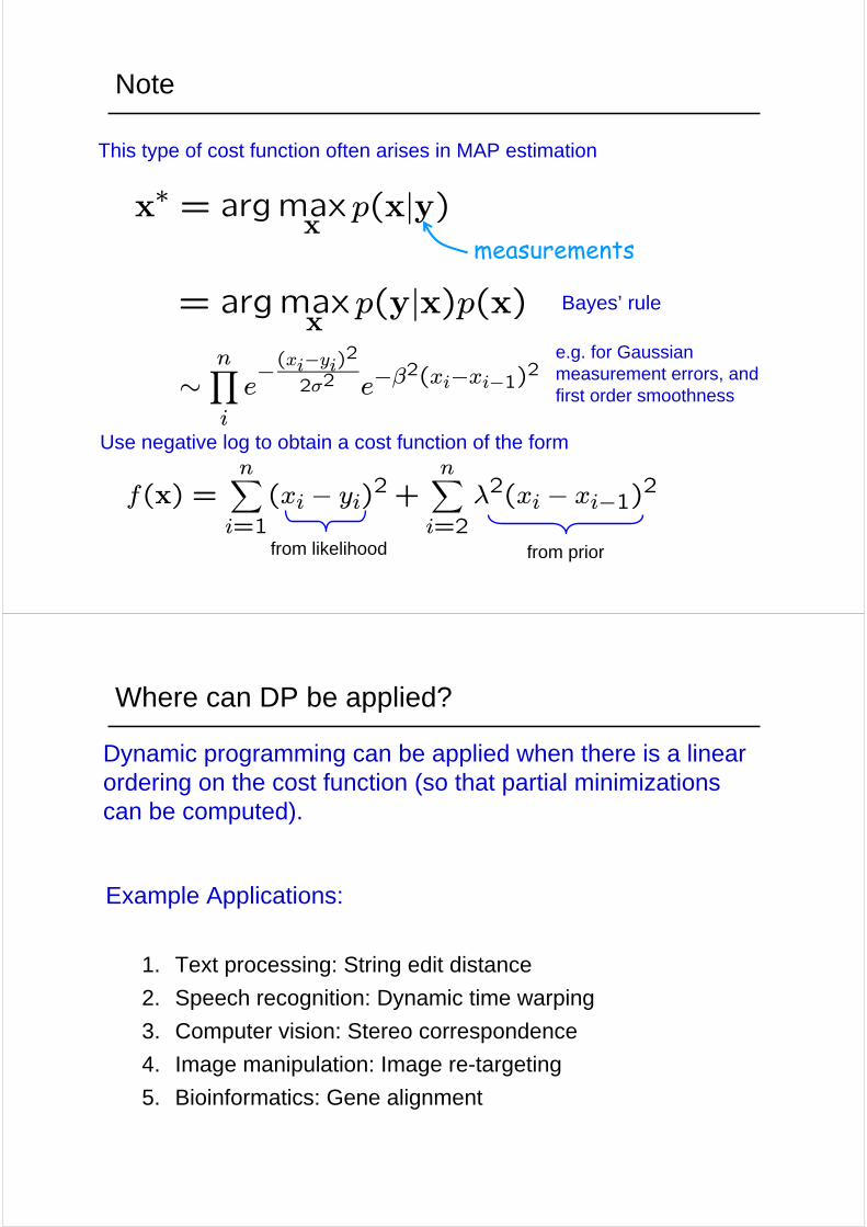
Note

This type of cost function often arises in MAP estimation

x∗ = argmaxxp(x|y)

measurements

= argmaxxp(y|x)p(x) Bayes’ rule

e.g. for Gaussian measurement errors, and first order smoothness

Use negative log to obtain a cost function of the form

from likelihood from prior

f(x) =nXi=1

(xi − yi)2 +nXi=2

λ2(xi − xi−1)2

∼nYi

e−(xi−yi)

2

2σ2 e−β2(xi−xi−1)2

Where can DP be applied?

Example Applications:

1. Text processing: String edit distance

2. Speech recognition: Dynamic time warping

3. Computer vision: Stereo correspondence

4. Image manipulation: Image re-targeting

5. Bioinformatics: Gene alignment

Dynamic programming can be applied when there is a linear ordering on the cost function (so that partial minimizations can be computed).

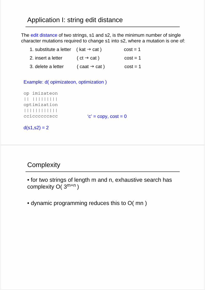
Application I: string edit distance

The edit distance of two strings, s1 and s2, is the minimum number of single character mutations required to change s1 into s2, where a mutation is one of:

1. substitute a letter ( kat cat ) cost = 1

2. insert a letter ( ct cat ) cost = 1

3. delete a letter ( caat cat ) cost = 1

Example: d( opimizateon, optimization )

op imizateon|| |||||||||optimization||||||||||||cciccccccscc

d(s1,s2) = 2

‘c’ = copy, cost = 0

Complexity

• for two strings of length m and n, exhaustive search has complexity O( 3m+n )

• dynamic programming reduces this to O( mn )

Using string edit distance for spelling correction

1. Check if word w is in the dictionary D

2. If it is not, then find the word x in D that minimizes d(w, x)

3. Suggest x as the corrected spelling for w

Note: step 2 appears to require computing the edit distance to all words in D, but this is not required at run time because edit distance is a metric, and this allows efficient search.

0 1 2 3 4 5 6-0.4

-0.3

-0.2

-0.1

0

0.1

0.2

0.3

0.4

0.5

0 1 2 3 4 5-0.4

-0.3

-0.2

-0.1

0

0.1

0.2

0.3

0.4

0.5

50 100 150 200 250 300 350 400

50

100

150

200

250

50 100 150 200 250 300 350

50

100

150

200

250

audio

log(STFT)

time

short term Fourier transform

sample template

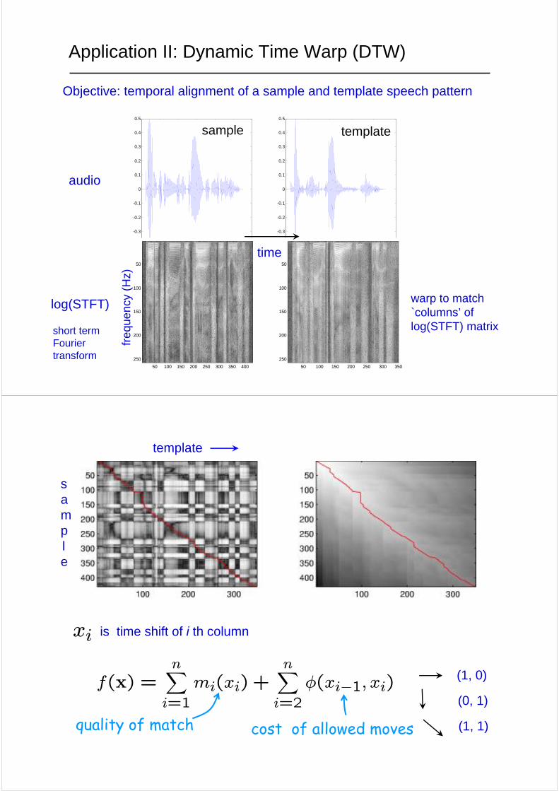
Application II: Dynamic Time Warp (DTW)

Objective: temporal alignment of a sample and template speech pattern

freq

uenc

y (H

z)

warp to match `columns’ of log(STFT) matrix

Application II: Dynamic Time Warp (DTW)

is time shift of i th column

quality of match cost of allowed moves

f(x) =nXi=1

mi(xi) +nXi=2

φ(xi−1, xi)

template

sample

(1, 0)

(0, 1)

(1, 1)

xi

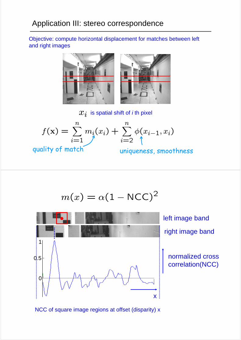
Application III: stereo correspondence

Objective: compute horizontal displacement for matches between left and right images

quality of match uniqueness, smoothness

f(x) =nXi=1

mi(xi) +nXi=2

φ(xi−1, xi)

is spatial shift of i th pixelxi

left image band

right image band

normalized cross correlation(NCC)

1

0

0.5

x

m(x) = α(1−NCC)2

NCC of square image regions at offset (disparity) x

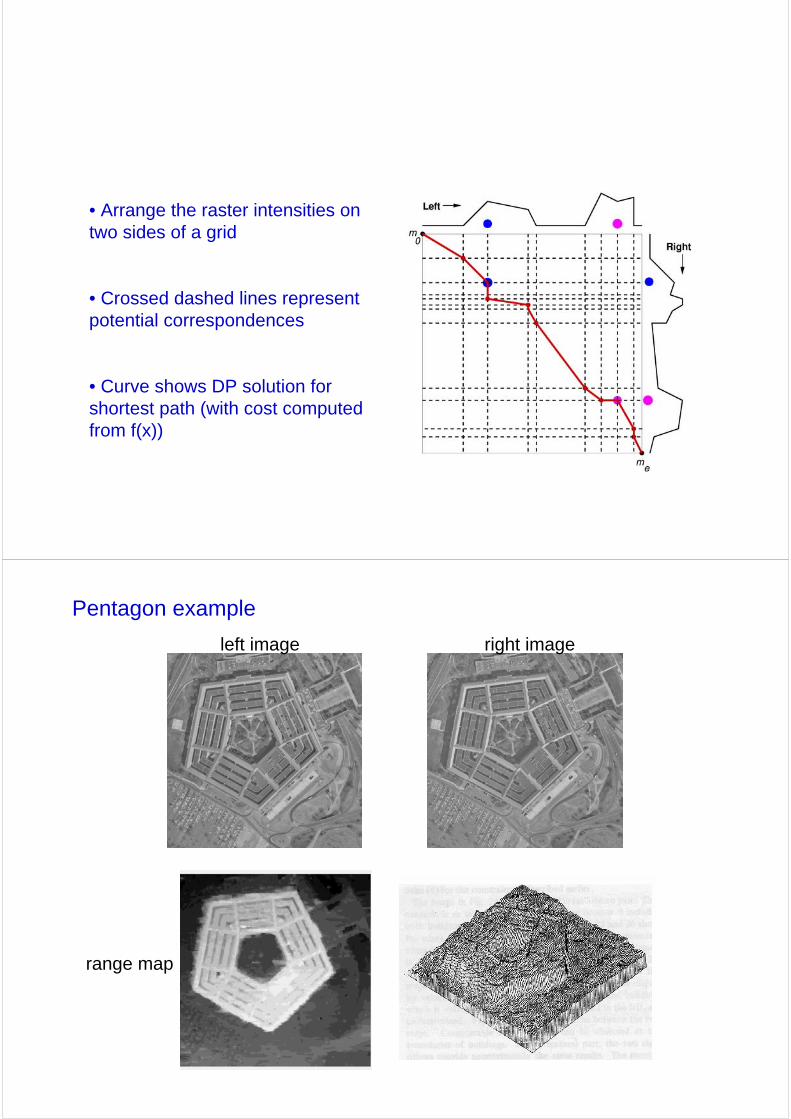
• Arrange the raster intensities on two sides of a grid

• Crossed dashed lines represent potential correspondences

• Curve shows DP solution for shortest path (with cost computed from f(x))

range map

Pentagon example

left image right image

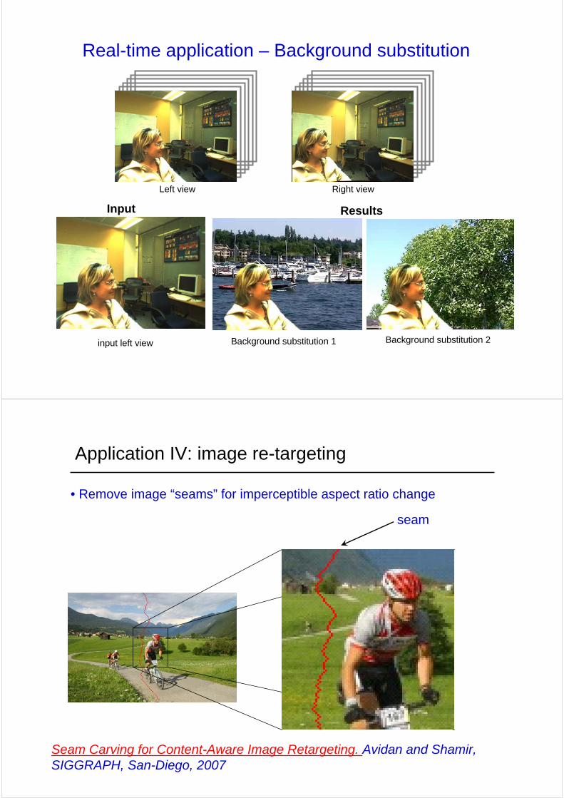
Real-time application – Background substitution

Left view Right view

Input

input left view

Results

Background substitution 1 Background substitution 2

• Remove image “seams” for imperceptible aspect ratio change

Application IV: image re-targeting

seam

Seam Carving for Content-Aware Image Retargeting. Avidan and Shamir, SIGGRAPH, San-Diego, 2007

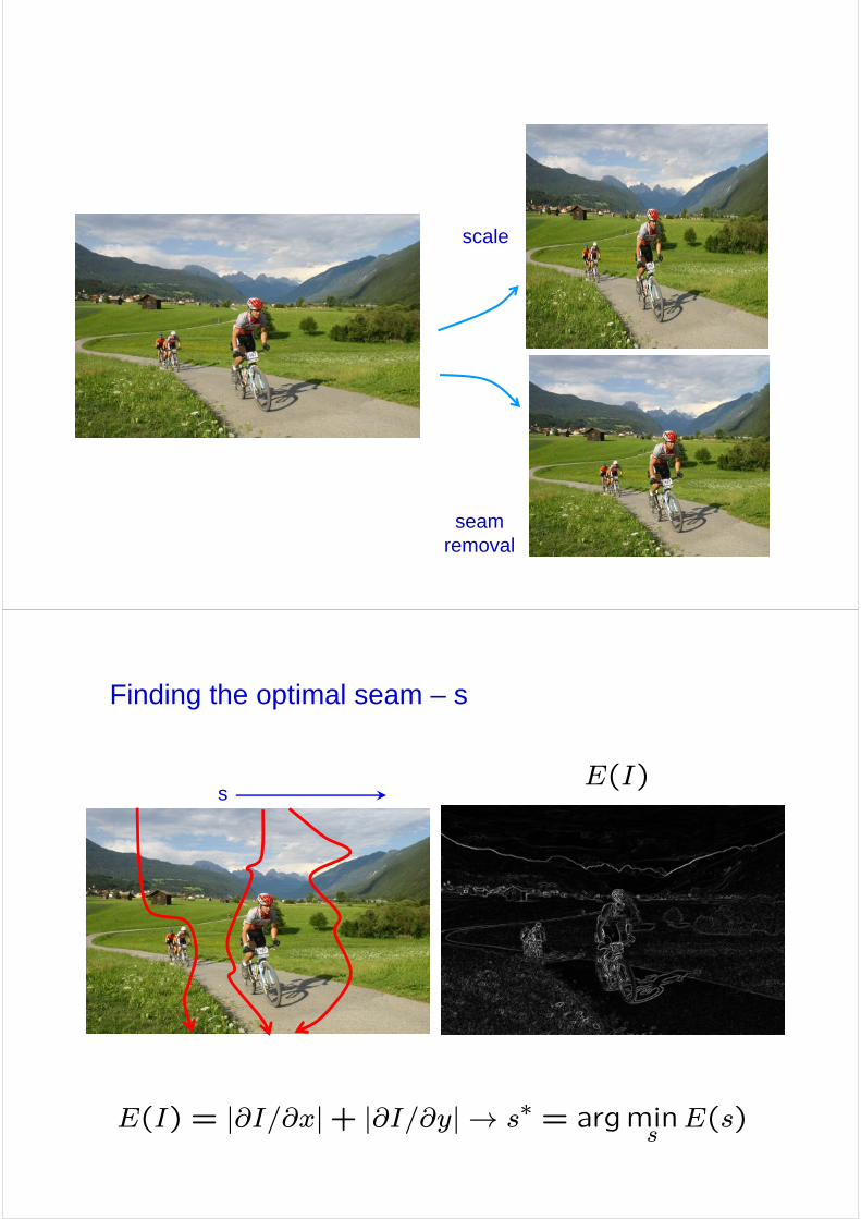
scale

seam removal

Finding the optimal seam – s

E(I) = |∂I/∂x|+ |∂I/∂y|→ s∗ = argminsE(s)

E(I)s