Numerical Linear Algebra - School of Statistics : … Linear Algebra Charles J. Geyer School of...
46
Numerical Linear Algebra Charles J. Geyer School of Statistics University of Minnesota Stat 8054 Lecture Notes 1
Transcript of Numerical Linear Algebra - School of Statistics : … Linear Algebra Charles J. Geyer School of...
Numerical Linear Algebra
Charles J. Geyer
School of Statistics
University of Minnesota
Stat 8054 Lecture Notes
1
Numerical Linear Algebra is about
• solving linear equations
• matrix factorizations
• eigenvalues and eigenvectors
2
Before We Begin
One thing you never want to do is matrix inversion.
Think of it as solving linear equations instead. Not
β̂ = (XTX)−1XTy
Rather, β̂ is the solution of
XTXβ = XTy
3
Gaussian Elimination
Gaussian elimination is how you were taught to solve systems oflinear equations in high school.
• Solve one equation for one variable in terms of the rest.
• Plug that solution into the rest of the equations.
• The rest of the equations are now a system of equations withone less variable.
• Repeat.
4
Gaussian Elimination (cont.)
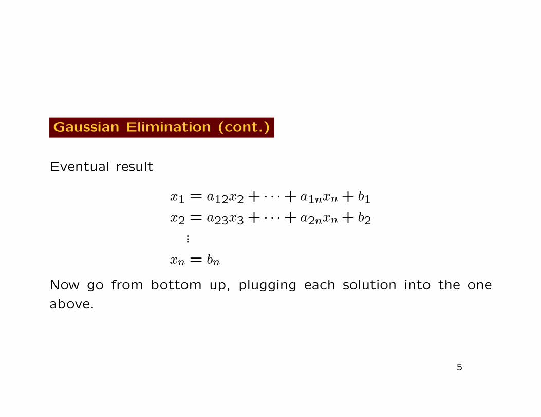
Eventual result
x1 = a12x2 + · · ·+ a1nxn + b1
x2 = a23x3 + · · ·+ a2nxn + b2...
xn = bn
Now go from bottom up, plugging each solution into the one
above.
5
LU Decomposition
The mathematical abstraction corresponding to Gaussian elimi-
nation is LU decomposition
M = LU
where L is lower triangular and U is upper triangular.
Triangular matrices are easy to invert or to solve, essentially
the plug-in on the preceding page, more formally called back
substitution.
6
Pivoting
LU decomposition can be very unstable (have large errors due
to inexactness of computer arithmetic) if done without pivoting
(carefully choosing the order in which variables are eliminated).
A permutation matrix P is an identity matrix whose rows have
been permuted. It contains exactly one 1 in each row and each
column.
Pivoting means we factor PM , which is M with rows permuted
(row pivoting), or MP , which is M with columns permuted (col-
umn pivoting).
7
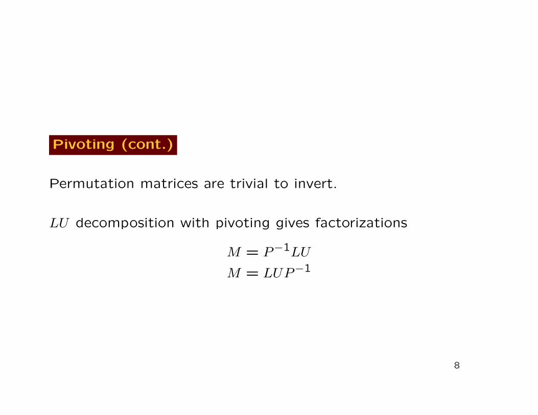
Pivoting (cont.)
Permutation matrices are trivial to invert.
LU decomposition with pivoting gives factorizations
M = P−1LU
M = LUP−1
8
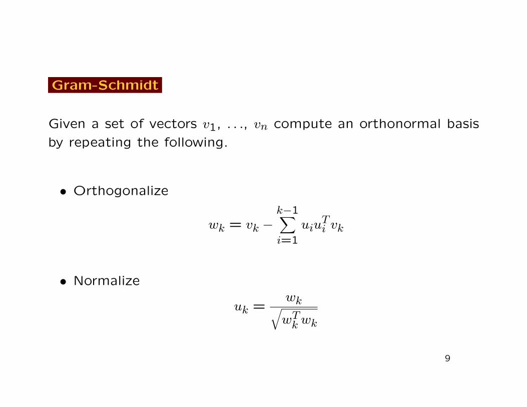
Gram-Schmidt
Given a set of vectors v1, . . ., vn compute an orthonormal basis
by repeating the following.
• Orthogonalize
wk = vk −k−1∑i=1
uiuTi vk
• Normalize
uk =wk√wTk wk
9
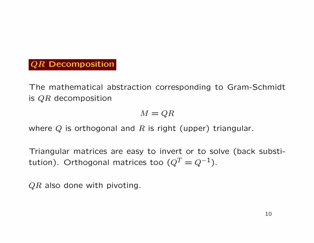
QR Decomposition
The mathematical abstraction corresponding to Gram-Schmidt
is QR decomposition
M = QR
where Q is orthogonal and R is right (upper) triangular.
Triangular matrices are easy to invert or to solve (back substi-
tution). Orthogonal matrices too (QT = Q−1).
QR also done with pivoting.
10
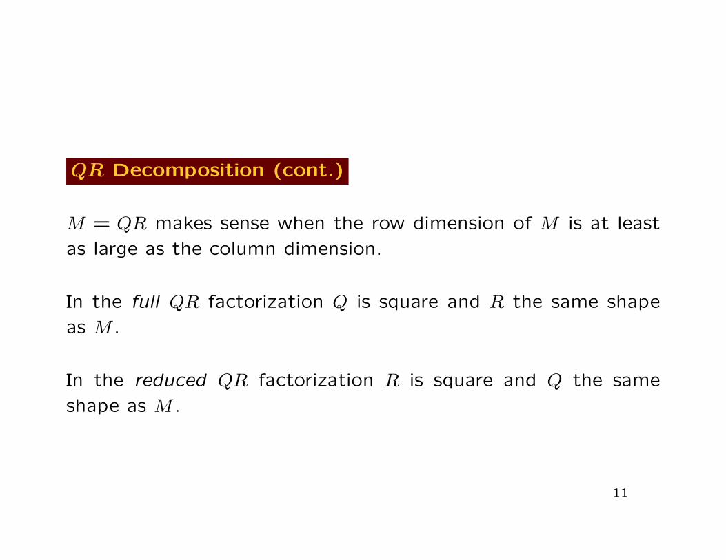
QR Decomposition (cont.)
M = QR makes sense when the row dimension of M is at least
as large as the column dimension.
In the full QR factorization Q is square and R the same shape
as M .
In the reduced QR factorization R is square and Q the same
shape as M .
11
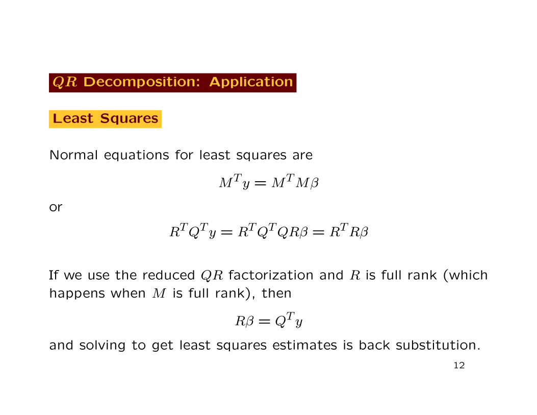
QR Decomposition: Application
Least Squares
Normal equations for least squares are
MTy = MTMβ
or
RTQTy = RTQTQRβ = RTRβ
If we use the reduced QR factorization and R is full rank (which
happens when M is full rank), then
Rβ = QTy
and solving to get least squares estimates is back substitution.
12
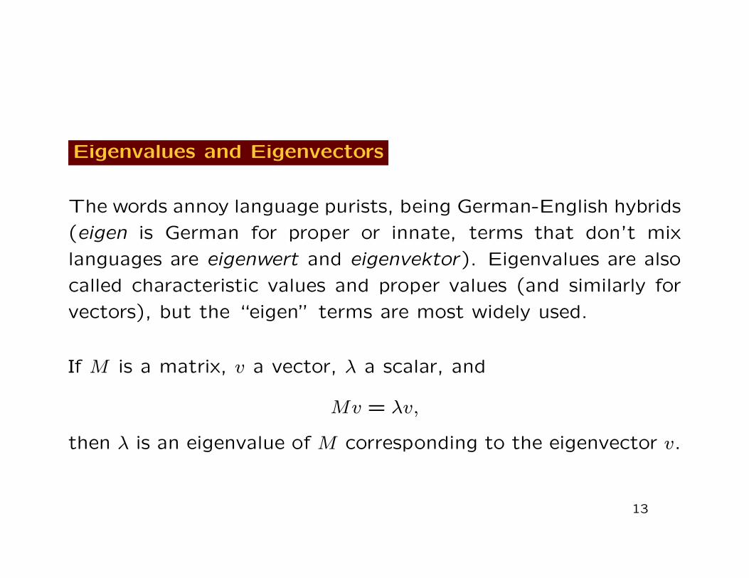
Eigenvalues and Eigenvectors
The words annoy language purists, being German-English hybrids
(eigen is German for proper or innate, terms that don’t mix
languages are eigenwert and eigenvektor). Eigenvalues are also
called characteristic values and proper values (and similarly for
vectors), but the “eigen” terms are most widely used.
If M is a matrix, v a vector, λ a scalar, and
Mv = λv,
then λ is an eigenvalue of M corresponding to the eigenvector v.
13
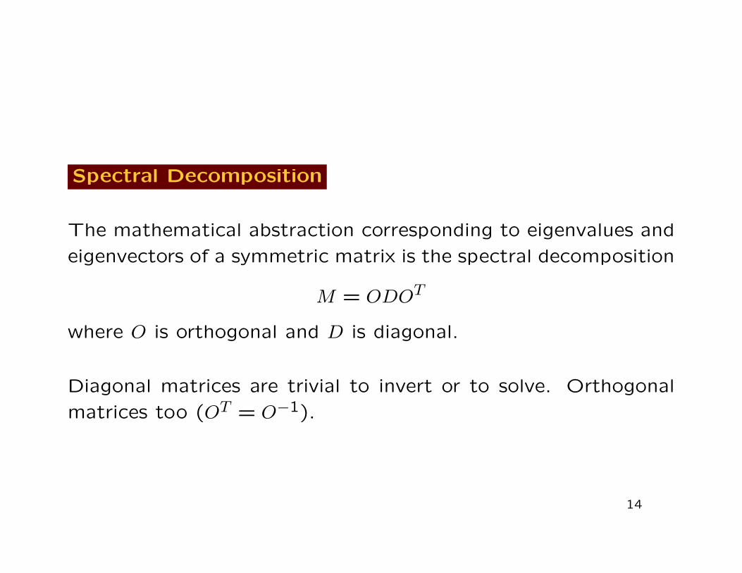
Spectral Decomposition
The mathematical abstraction corresponding to eigenvalues and
eigenvectors of a symmetric matrix is the spectral decomposition
M = ODOT
where O is orthogonal and D is diagonal.
Diagonal matrices are trivial to invert or to solve. Orthogonal
matrices too (OT = O−1).
14
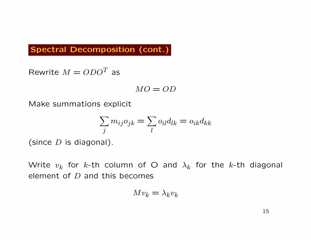
Spectral Decomposition (cont.)
Rewrite M = ODOT as
MO = OD
Make summations explicit∑j
mijojk =∑l
oildlk = oikdkk
(since D is diagonal).
Write vk for k-th column of O and λk for the k-th diagonal
element of D and this becomes
Mvk = λkvk
15
Spectral Decomposition (cont.)
Conclusion: the spectral decomposition theorem asserts that
every symmetric n × n matrix has n eigenvectors that make up
an orthonormal basis.
16
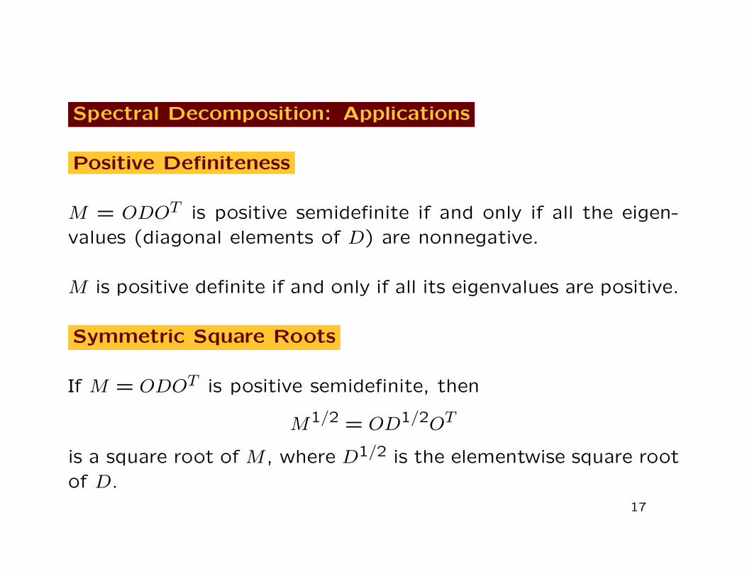
Spectral Decomposition: Applications
Positive Definiteness
M = ODOT is positive semidefinite if and only if all the eigen-values (diagonal elements of D) are nonnegative.
M is positive definite if and only if all its eigenvalues are positive.
Symmetric Square Roots
If M = ODOT is positive semidefinite, then
M1/2 = OD1/2OT
is a square root of M , where D1/2 is the elementwise square rootof D.
17
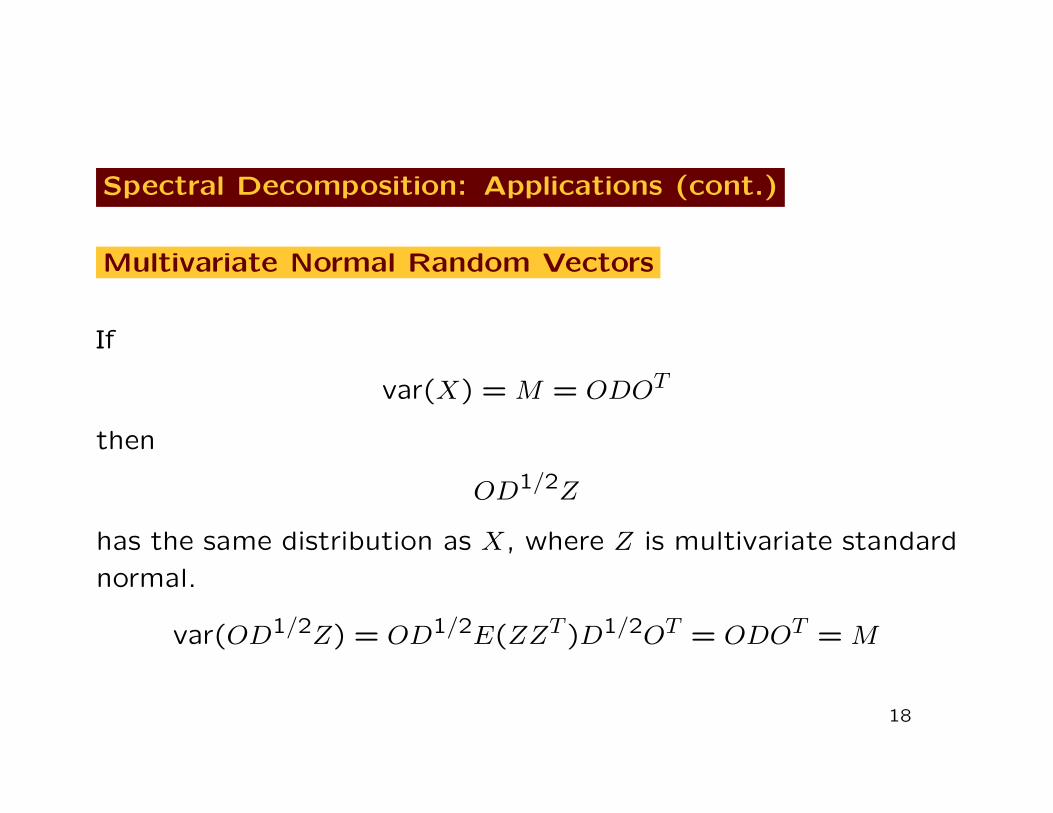
Spectral Decomposition: Applications (cont.)
Multivariate Normal Random Vectors
If
var(X) = M = ODOT
then
OD1/2Z
has the same distribution as X, where Z is multivariate standard
normal.
var(OD1/2Z) = OD1/2E(ZZT )D1/2OT = ODOT = M
18
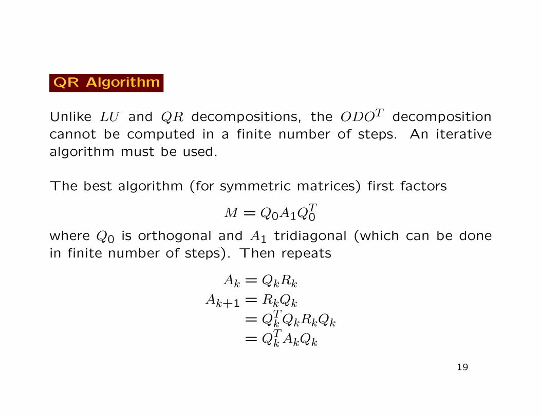
QR Algorithm
Unlike LU and QR decompositions, the ODOT decompositioncannot be computed in a finite number of steps. An iterativealgorithm must be used.
The best algorithm (for symmetric matrices) first factors
M = Q0A1QT0
where Q0 is orthogonal and A1 tridiagonal (which can be donein finite number of steps). Then repeats
Ak = QkRkAk+1 = RkQk
= QTkQkRkQk= QTkAkQk
19
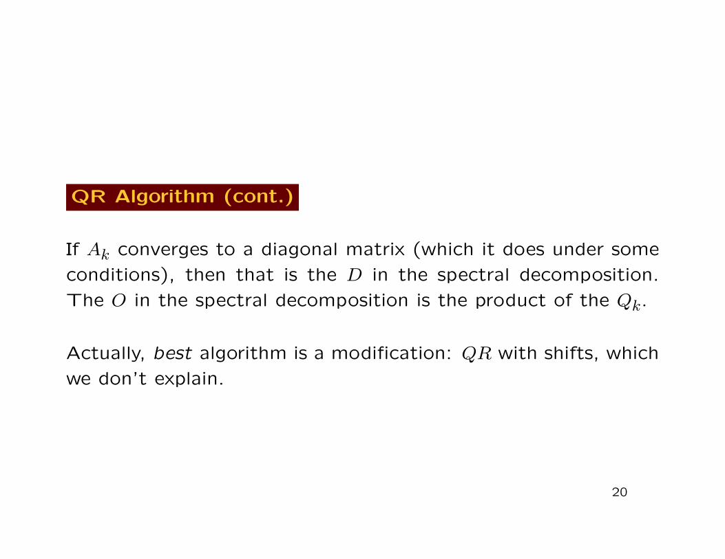
QR Algorithm (cont.)
If Ak converges to a diagonal matrix (which it does under some
conditions), then that is the D in the spectral decomposition.
The O in the spectral decomposition is the product of the Qk.
Actually, best algorithm is a modification: QR with shifts, which
we don’t explain.
20
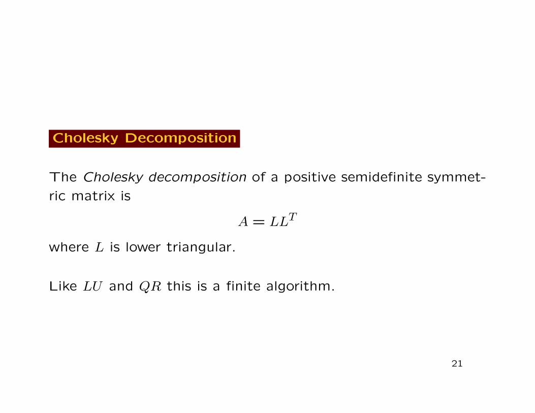
Cholesky Decomposition
The Cholesky decomposition of a positive semidefinite symmet-
ric matrix is
A = LLT
where L is lower triangular.
Like LU and QR this is a finite algorithm.
21
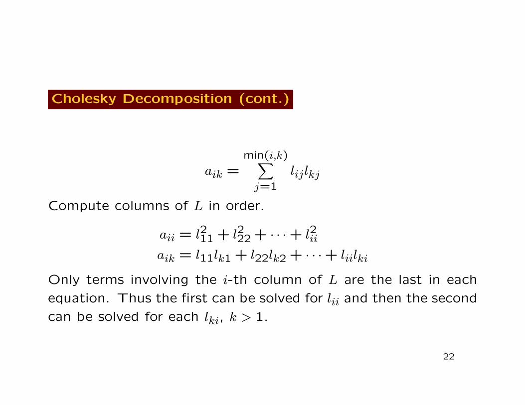
Cholesky Decomposition (cont.)
aik =min(i,k)∑j=1
lijlkj
Compute columns of L in order.
aii = l211 + l222 + · · ·+ l2ii
aik = l11lk1 + l22lk2 + · · ·+ liilki
Only terms involving the i-th column of L are the last in each
equation. Thus the first can be solved for lii and then the second
can be solved for each lki, k > 1.
22
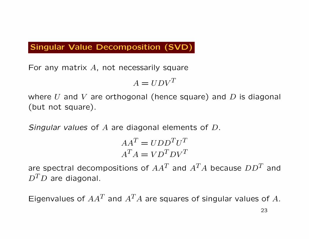
Singular Value Decomposition (SVD)
For any matrix A, not necessarily square
A = UDV T
where U and V are orthogonal (hence square) and D is diagonal(but not square).
Singular values of A are diagonal elements of D.
AAT = UDDTUT
ATA = V DTDV T
are spectral decompositions of AAT and ATA because DDT andDTD are diagonal.
Eigenvalues of AAT and ATA are squares of singular values of A.
23
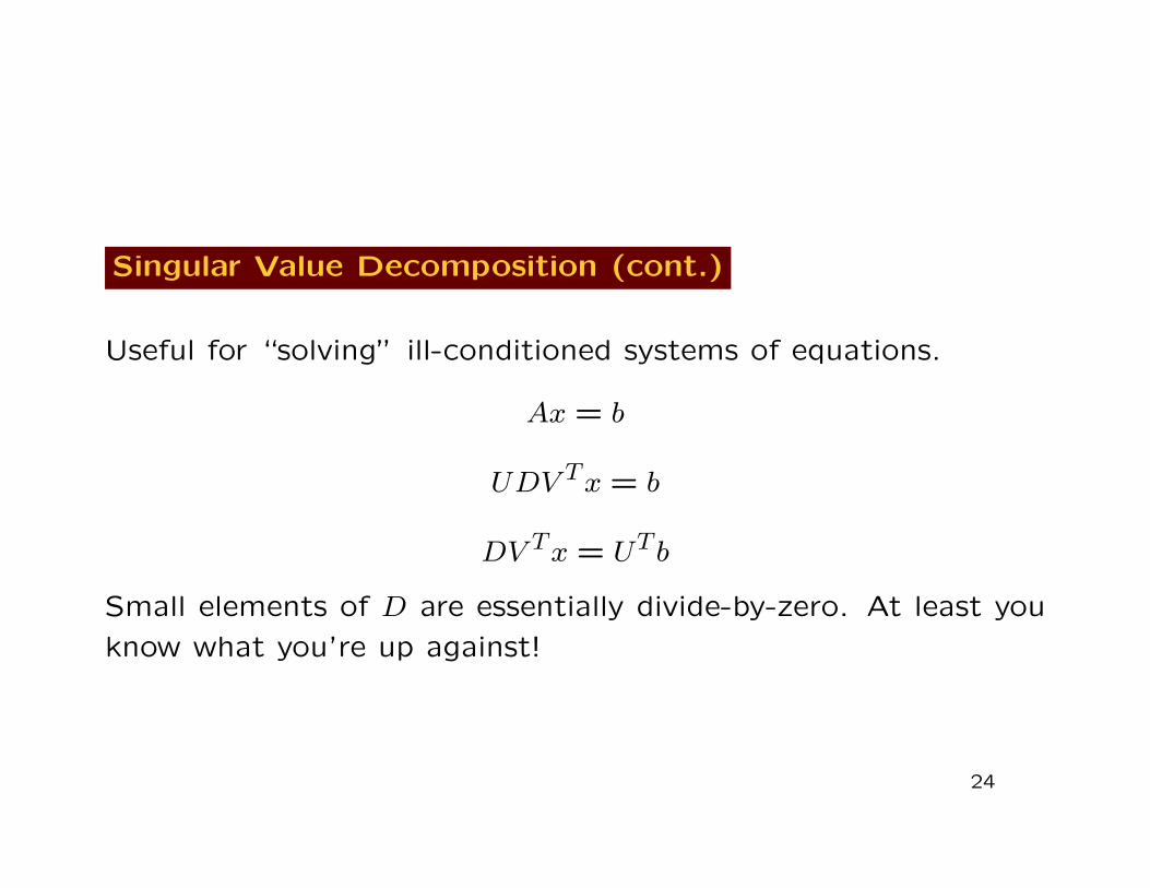
Singular Value Decomposition (cont.)
Useful for “solving” ill-conditioned systems of equations.
Ax = b
UDV Tx = b
DV Tx = UT b
Small elements of D are essentially divide-by-zero. At least you
know what you’re up against!
24
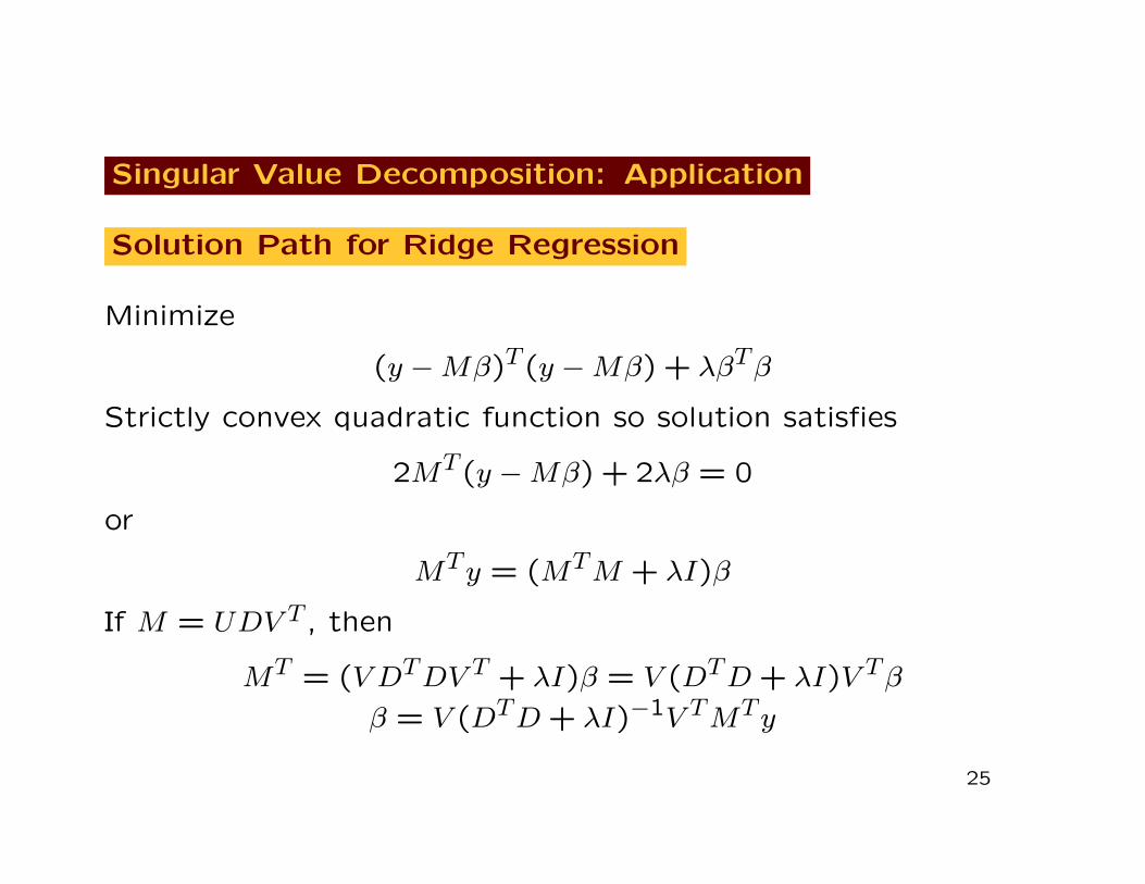
Singular Value Decomposition: Application
Solution Path for Ridge Regression
Minimize
(y −Mβ)T (y −Mβ) + λβTβ
Strictly convex quadratic function so solution satisfies
2MT (y −Mβ) + 2λβ = 0
or
MTy = (MTM + λI)β
If M = UDV T , then
MT = (V DTDV T + λI)β = V (DTD + λI)V Tβ
β = V (DTD + λI)−1V TMTy
25
Summary of Old Stuff
Methods for non-square complex matrices: SVD and QR.
Methods for square complex matrices: LU , eigenvalue-eigenvector
(latter does not work for some matrices).
Methods for square positive semidefinite real matrices: LLT .
26
A Really Good Reference
Trefethen and Bau
Numerical Linear Algebra
SIAM, 1997
27
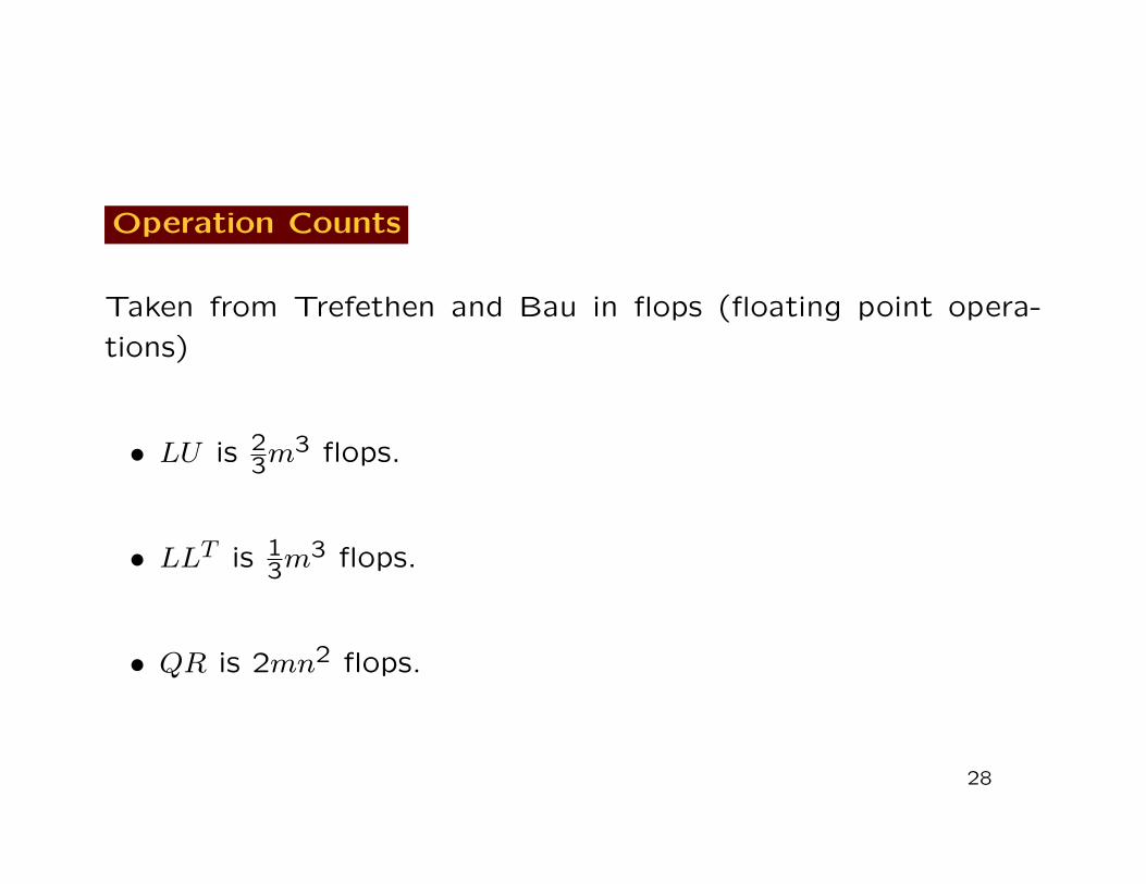
Operation Counts
Taken from Trefethen and Bau in flops (floating point opera-
tions)
• LU is 23m
3 flops.
• LLT is 13m
3 flops.
• QR is 2mn2 flops.
28
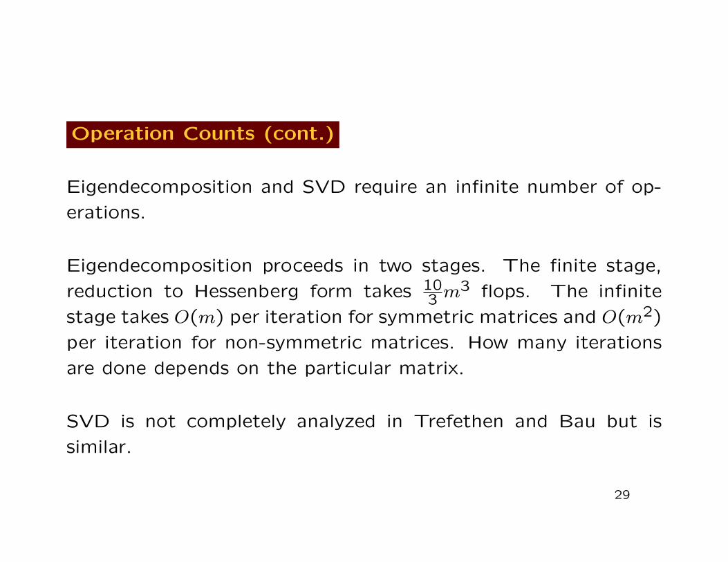
Operation Counts (cont.)
Eigendecomposition and SVD require an infinite number of op-
erations.
Eigendecomposition proceeds in two stages. The finite stage,
reduction to Hessenberg form takes 103 m
3 flops. The infinite
stage takes O(m) per iteration for symmetric matrices and O(m2)
per iteration for non-symmetric matrices. How many iterations
are done depends on the particular matrix.
SVD is not completely analyzed in Trefethen and Bau but is
similar.
29

Break
Preceding stuff is the basics.
Now for some fancier stuff.
30
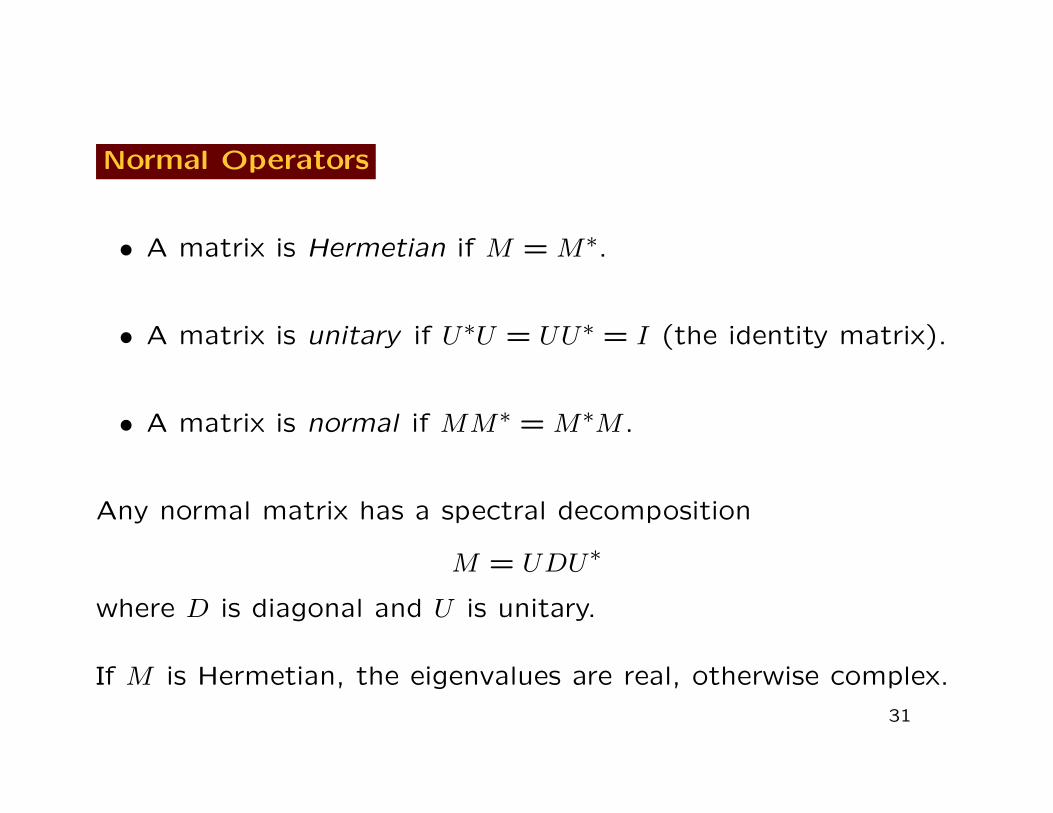
Normal Operators
• A matrix is Hermetian if M = M∗.
• A matrix is unitary if U∗U = UU∗ = I (the identity matrix).
• A matrix is normal if MM∗ = M∗M .
Any normal matrix has a spectral decomposition
M = UDU∗
where D is diagonal and U is unitary.
If M is Hermetian, the eigenvalues are real, otherwise complex.
31
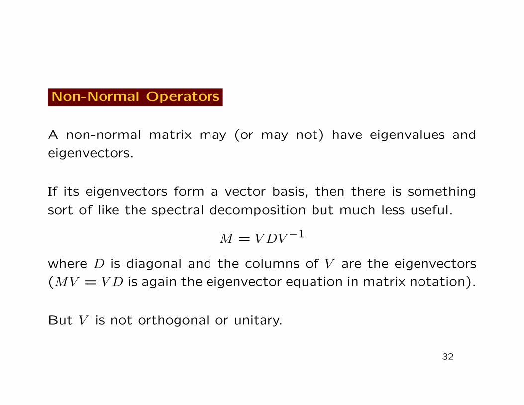
Non-Normal Operators
A non-normal matrix may (or may not) have eigenvalues and
eigenvectors.
If its eigenvectors form a vector basis, then there is something
sort of like the spectral decomposition but much less useful.
M = V DV −1
where D is diagonal and the columns of V are the eigenvectors
(MV = V D is again the eigenvector equation in matrix notation).
But V is not orthogonal or unitary.
32
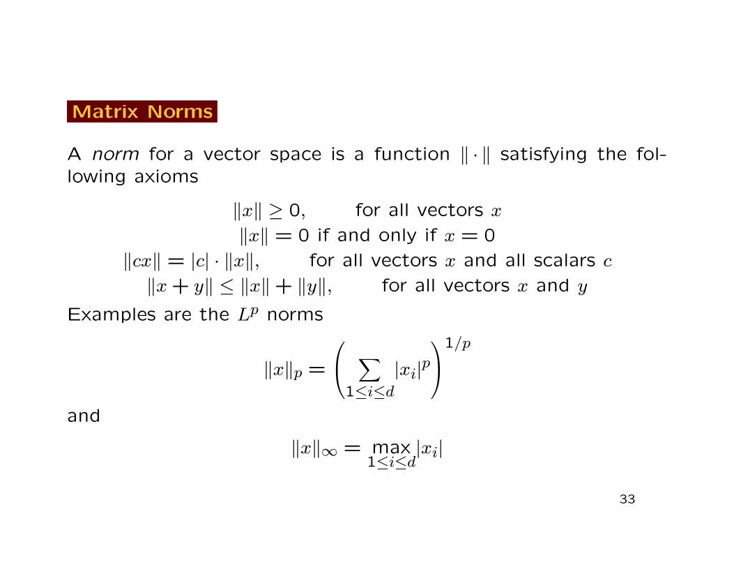
Matrix Norms
A norm for a vector space is a function ‖ · ‖ satisfying the fol-lowing axioms
‖x‖ ≥ 0, for all vectors x
‖x‖ = 0 if and only if x = 0
‖cx‖ = |c| · ‖x‖, for all vectors x and all scalars c
‖x+ y‖ ≤ ‖x‖+ ‖y‖, for all vectors x and y
Examples are the Lp norms
‖x‖p =
∑1≤i≤d
|xi|p1/p
and
‖x‖∞ = max1≤i≤d
|xi|
33
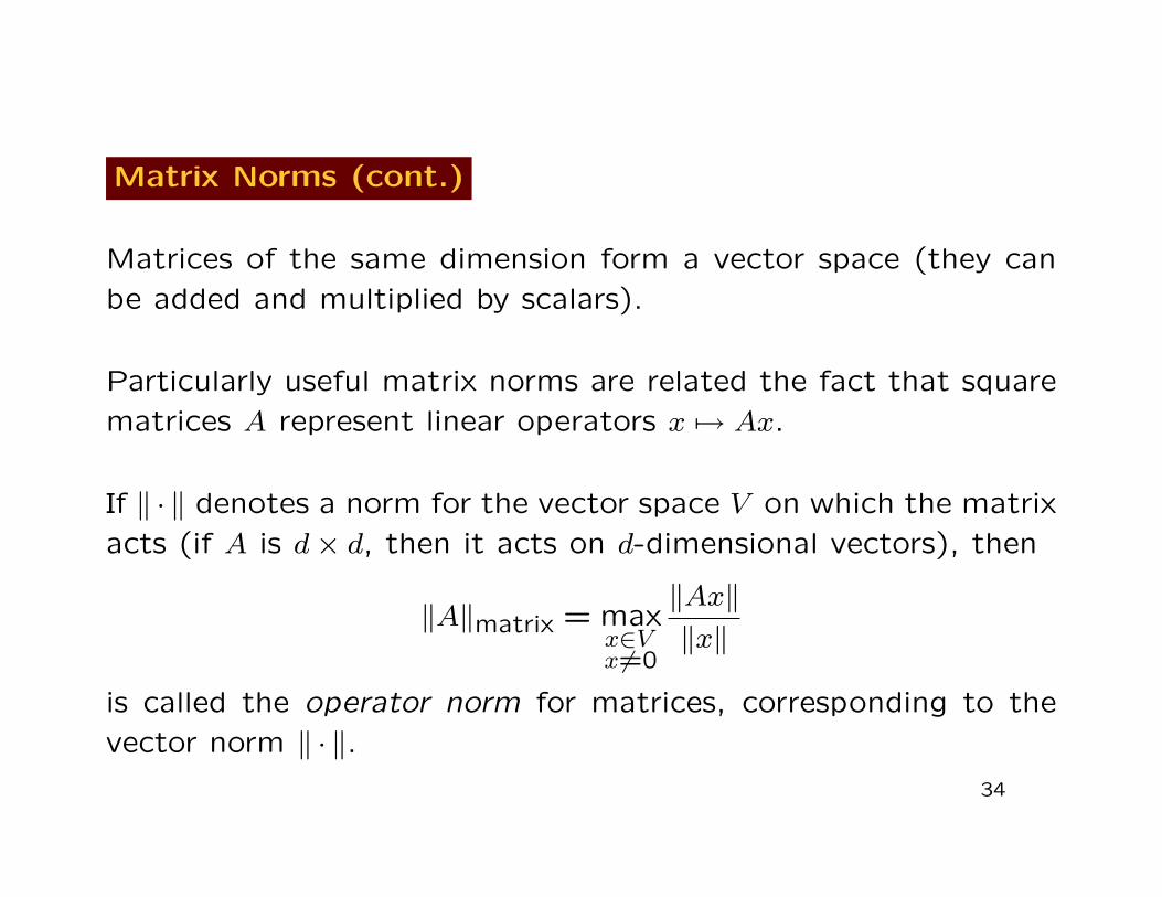
Matrix Norms (cont.)
Matrices of the same dimension form a vector space (they can
be added and multiplied by scalars).
Particularly useful matrix norms are related the fact that square
matrices A represent linear operators x 7→ Ax.
If ‖ · ‖ denotes a norm for the vector space V on which the matrix
acts (if A is d× d, then it acts on d-dimensional vectors), then
‖A‖matrix = maxx∈Vx6=0
‖Ax‖‖x‖
is called the operator norm for matrices, corresponding to the
vector norm ‖ · ‖.34
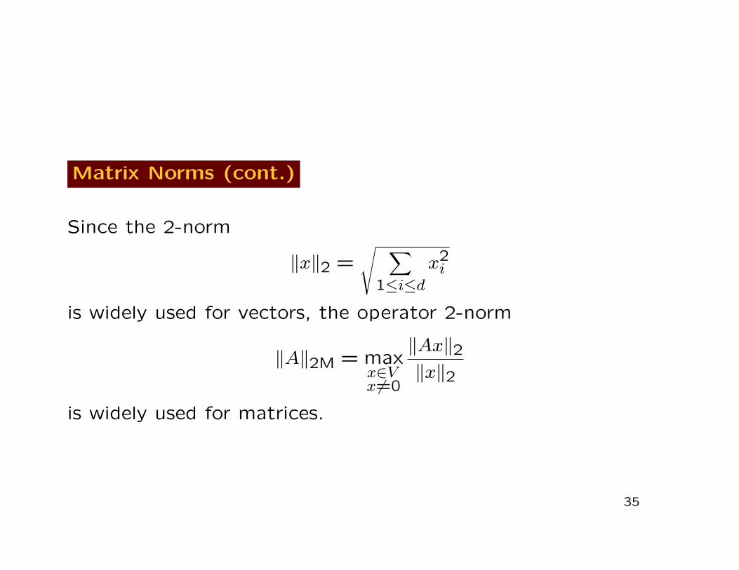
Matrix Norms (cont.)
Since the 2-norm
‖x‖2 =√ ∑
1≤i≤dx2i
is widely used for vectors, the operator 2-norm
‖A‖2M = maxx∈Vx6=0
‖Ax‖2‖x‖2
is widely used for matrices.
35
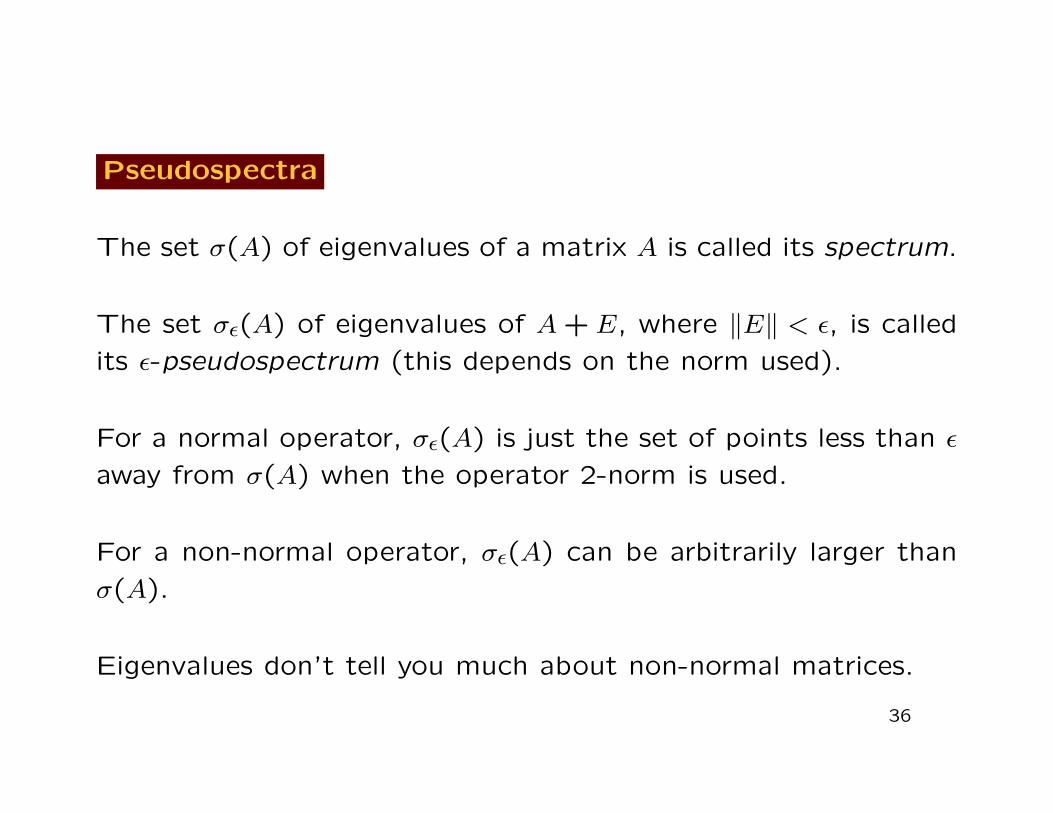
Pseudospectra
The set σ(A) of eigenvalues of a matrix A is called its spectrum.
The set σε(A) of eigenvalues of A + E, where ‖E‖ < ε, is called
its ε-pseudospectrum (this depends on the norm used).
For a normal operator, σε(A) is just the set of points less than ε
away from σ(A) when the operator 2-norm is used.
For a non-normal operator, σε(A) can be arbitrarily larger than
σ(A).
Eigenvalues don’t tell you much about non-normal matrices.
36
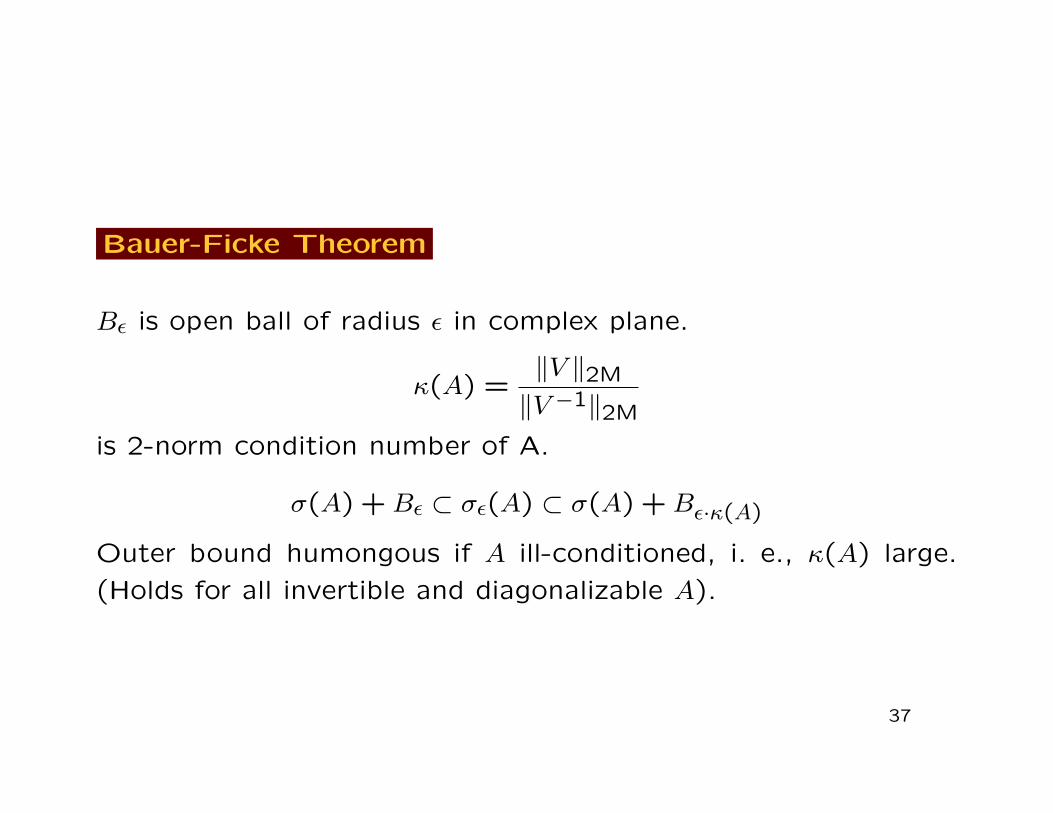
Bauer-Ficke Theorem
Bε is open ball of radius ε in complex plane.
κ(A) =‖V ‖2M
‖V −1‖2M
is 2-norm condition number of A.
σ(A) +Bε ⊂ σε(A) ⊂ σ(A) +Bε·κ(A)
Outer bound humongous if A ill-conditioned, i. e., κ(A) large.
(Holds for all invertible and diagonalizable A).
37
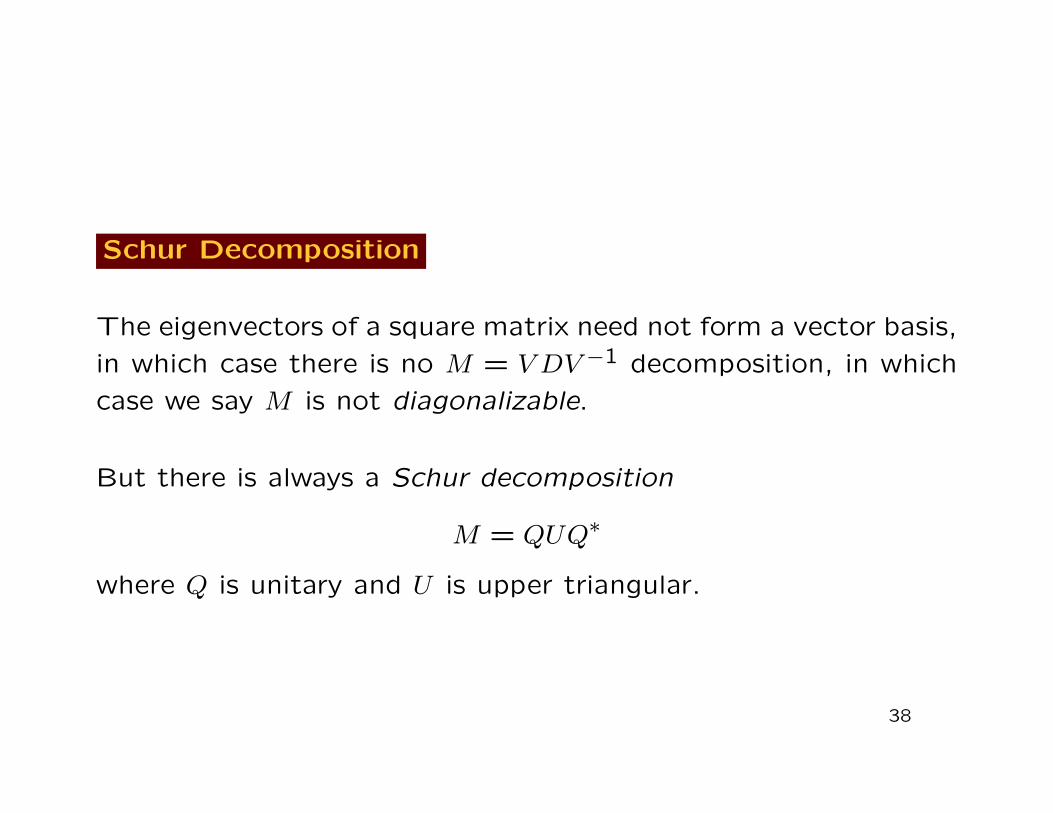
Schur Decomposition
The eigenvectors of a square matrix need not form a vector basis,
in which case there is no M = V DV −1 decomposition, in which
case we say M is not diagonalizable.
But there is always a Schur decomposition
M = QUQ∗
where Q is unitary and U is upper triangular.
38
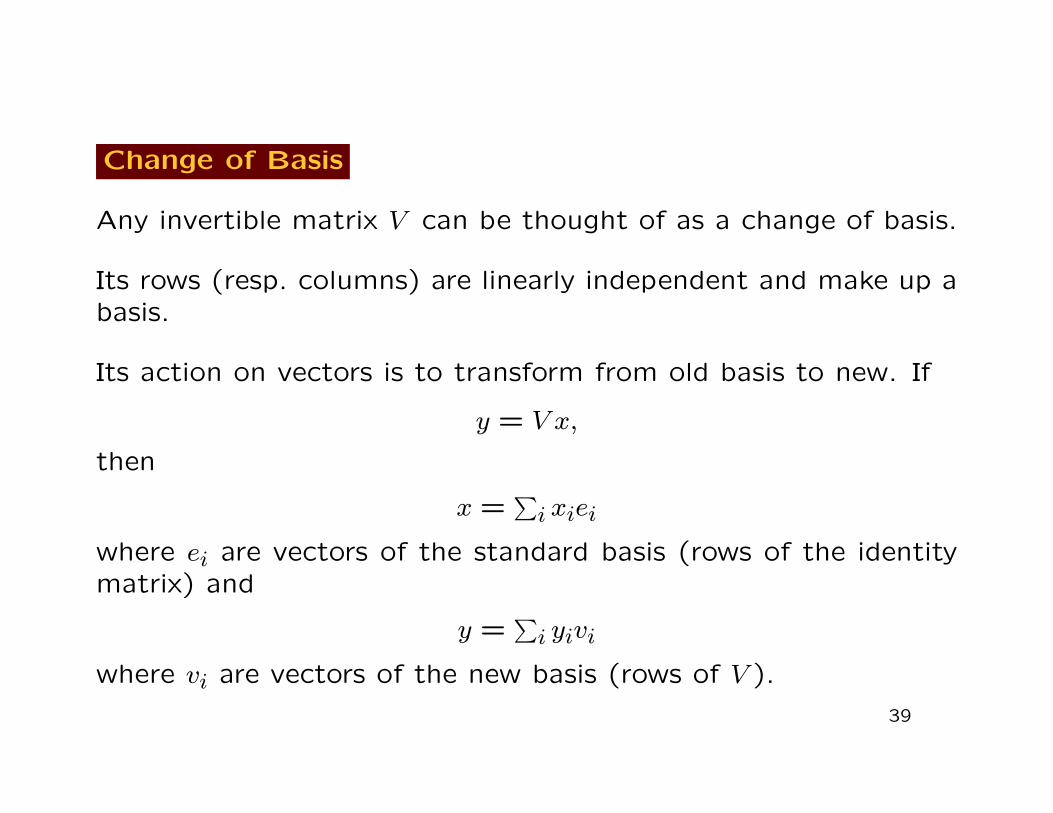
Change of Basis
Any invertible matrix V can be thought of as a change of basis.
Its rows (resp. columns) are linearly independent and make up abasis.
Its action on vectors is to transform from old basis to new. If
y = V x,
then
x =∑i xiei
where ei are vectors of the standard basis (rows of the identitymatrix) and
y =∑i yivi
where vi are vectors of the new basis (rows of V ).
39
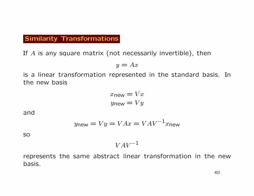
Similarity Transformations
If A is any square matrix (not necessarily invertible), then
y = Ax
is a linear transformation represented in the standard basis. Inthe new basis
xnew = V x
ynew = V y
and
ynew = V y = V Ax = V AV −1xnew
so
V AV −1
represents the same abstract linear transformation in the newbasis.
40
Similarity Transformations (cont.)
A 7→ V AV −1 is called a similarity transformation.
A and V AV −1 are similar matrices.
41
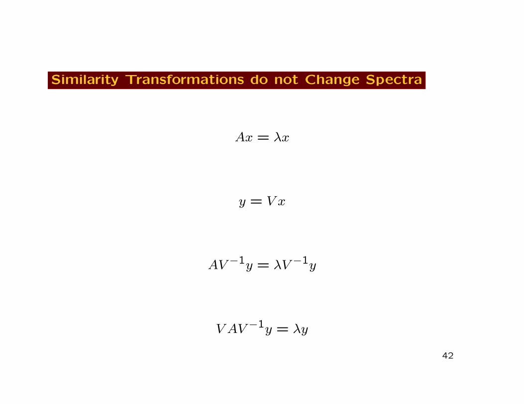
Similarity Transformations do not Change Spectra
Ax = λx
y = V x
AV −1y = λV −1y
V AV −1y = λy
42
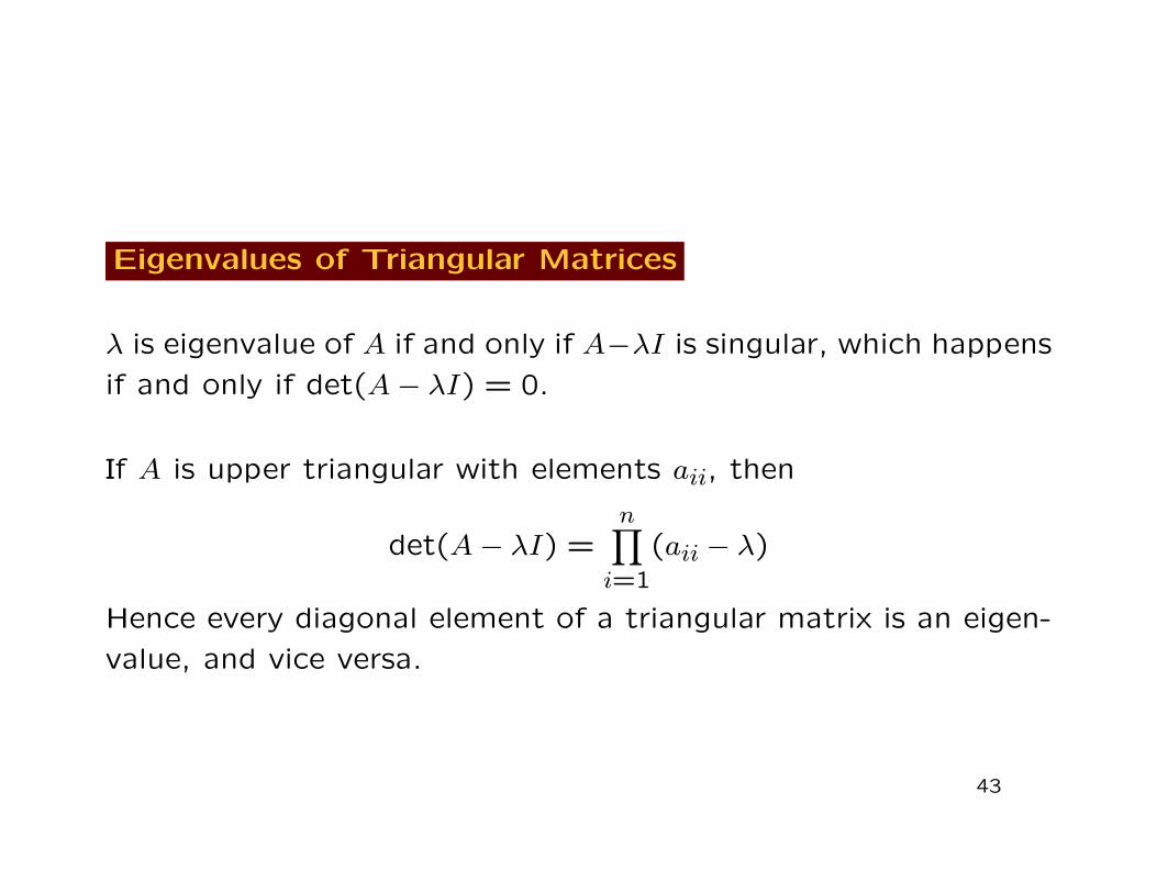
Eigenvalues of Triangular Matrices
λ is eigenvalue of A if and only if A−λI is singular, which happens
if and only if det(A− λI) = 0.
If A is upper triangular with elements aii, then
det(A− λI) =n∏i=1
(aii − λ)
Hence every diagonal element of a triangular matrix is an eigen-
value, and vice versa.
43
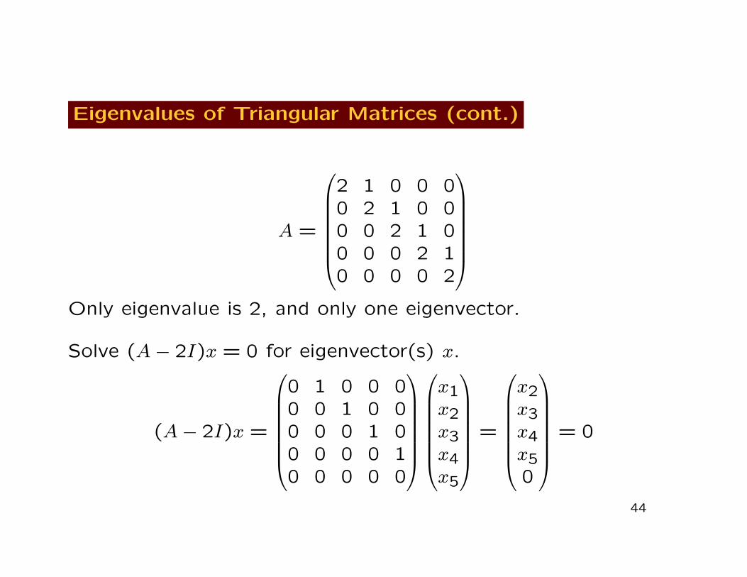
Eigenvalues of Triangular Matrices (cont.)
A =
2 1 0 0 00 2 1 0 00 0 2 1 00 0 0 2 10 0 0 0 2
Only eigenvalue is 2, and only one eigenvector.
Solve (A− 2I)x = 0 for eigenvector(s) x.
(A− 2I)x =
0 1 0 0 00 0 1 0 00 0 0 1 00 0 0 0 10 0 0 0 0
x1x2x3x4x5
=
x2x3x4x50
= 0
44
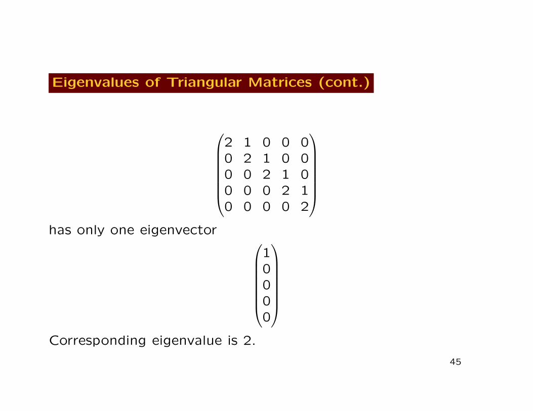
Eigenvalues of Triangular Matrices (cont.)
2 1 0 0 00 2 1 0 00 0 2 1 00 0 0 2 10 0 0 0 2
has only one eigenvector
10000
Corresponding eigenvalue is 2.
45
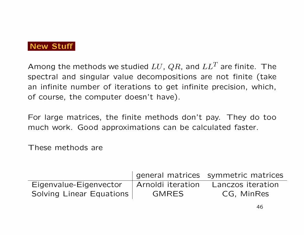
New Stuff
Among the methods we studied LU , QR, and LLT are finite. Thespectral and singular value decompositions are not finite (takean infinite number of iterations to get infinite precision, which,of course, the computer doesn’t have).
For large matrices, the finite methods don’t pay. They do toomuch work. Good approximations can be calculated faster.
These methods are
general matrices symmetric matricesEigenvalue-Eigenvector Arnoldi iteration Lanczos iterationSolving Linear Equations GMRES CG, MinRes
46
![Applied Numerical Linear Algebra. Lecture 10 · New York, 1959] or [P. Halmos. Finite Dimensional Vector Spaces. Van Nostrand, New York, 1958]. 4/47. Algorithms for the Nonsymmetric](https://static.fdocument.org/doc/165x107/5b5aeae57f8b9a302a8cd214/applied-numerical-linear-algebra-lecture-10-new-york-1959-or-p-halmos.jpg)