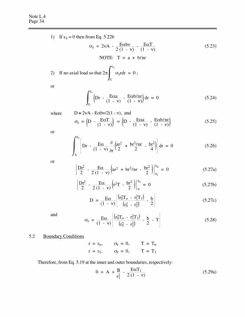
Rev 2001

22.312 ENGINEERING OF NUCLEAR REACTORS

Fall 2002

NOTE L.4

“INTRODUCTION TO STRUCTURAL MECHANICS”

Lothar Wolf*, Mujid S. Kazimi** and Neil E. Todreas†

σ2

σ1

Load Line

Shear Diagonal

35

-25

-57.7-60

-100

55 6569 100Nominal Load Point

Max τ theoryDE theoryMohr theoryMax σ theory

Limiting Points-45

* Professor of Nuclear Engineering (retired), University of Maryland** TEPCO Professor of Nuclear Engineering, Massachusetts Institute of Technology† KEPCO Professor of Nuclear Engineering, Massachusetts Institute of Technology

i

TABLE OF CONTENTS

Page

1. Definition of Concepts .......................................................................................................... 1

1.1 Concept of State of Stress ........................................................................................... 4

1.2 Principal Stresses, Planes and Directions .................................................................... 6

1.3 Basic Considerations of Strain ..................................................................................... 6

1.4 Plane Stress ................................................................................................................. 8

1.5 Mohr’s Circle...............................................................................................................10

1.6 Octahedral Planes and Stress........................................................................................13

1.7 Principal Strains and Planes .........................................................................................14

2. Elastic Stress-Strain Relations ..............................................................................................17

2.1 Generalized Hooke’s Law............................................................................................17

2.2 Modulus of Volume Expansion (Bulk Modulus) ........................................................19

3. Thin-Walled Cylinders and Sphere .......................................................................................21

3.1 Stresses .......................................................................................................................21

3.2 Deformation and Strains ..............................................................................................22

3.3 End Effects for the Closed-Ended Cylinder .................................................................24

4. Thick-Walled Cylinder under Radial Pressure ......................................................................27

4.1 Displacement Approach................................................................................................28

4.2 Stress Approach ...........................................................................................................29

5. Thermal Stress.......................................................................................................................31

5.1 Stress Distribution........................................................................................................32

5.2 Boundary Conditions ...................................................................................................34

5.3 Final Results.................................................................................................................32

6. Design Procedures ...............................................................................................................37

6.1 Static Failure and Failure Theories ...............................................................................38

6.2 Prediction of Failure under Biaxial and Triaxial Loading .............................................40

6.3 Maximum Normal-Stress Theory (Rankine) ...............................................................41

6.4 Maximum Shear Stress Theory (The Coulomb, later Tresca Theory)...........................44

6.5 Mohr Theory and Internal-Friction Theory ..................................................................46

6.6 Maximum Normal-Strain Theory (Saint-Varants’ Theory)..........................................47

6.7 Total Strain-Energy Theory (Beltrami Theory).............................................................48

6.8 Maximum Distortion-Energy Theory (Maximum Octahedral-Shear-StressTheory, Van Mises, Hencky) .......................................................................................49

ii

TABLE OF CONTENTS (continued)

Page

6.9 Comparison of Failure Theories .................................................................................51

6.10 Application of Failure Theories to Thick-Walled Cylinders........................................51

6.11 Prediction of Failure of Closed-Ended Circular Cylinder Thin-WalledPressure Vessels.........................................................................................................58

6.12 Examples for the Calculation of Safety Factors in Thin-Walled Cylinders.................60

References ...................................................................................................................................61

“INTRODUCTION TO STRUCTURAL MECHANICS”M. S. Kazimi, N.E. Todreas and L. Wolf

1. DEFINITION OF CONCEPTS

Structural mechanics is the body of knowledge describing the relations between external

forces, internal forces and deformation of structural materials. It is therefore necessary to clarify

the various terms that are commonly used to describe these quantities. In large part, structural

mechanics refers to solid mechanics because a solid is the only form of matter that can sustain

loads parallel to the surface. However, some considerations of fluid-like behavior (creep) are also

part of structural mechanics.

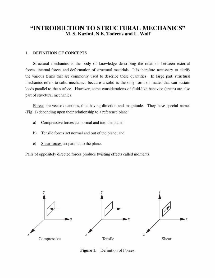
Forces are vector quantities, thus having direction and magnitude. They have special names

(Fig. 1) depending upon their relationship to a reference plane:

a) Compressive forces act normal and into the plane;

b) Tensile forces act normal and out of the plane; and

c) Shear forces act parallel to the plane.

Pairs of oppositely directed forces produce twisting effects called moments.

y

x

z

y

x

z

y

x

zCompressive Tensile Shear

Figure 1. Definition of Forces.

Note L.4Page 2

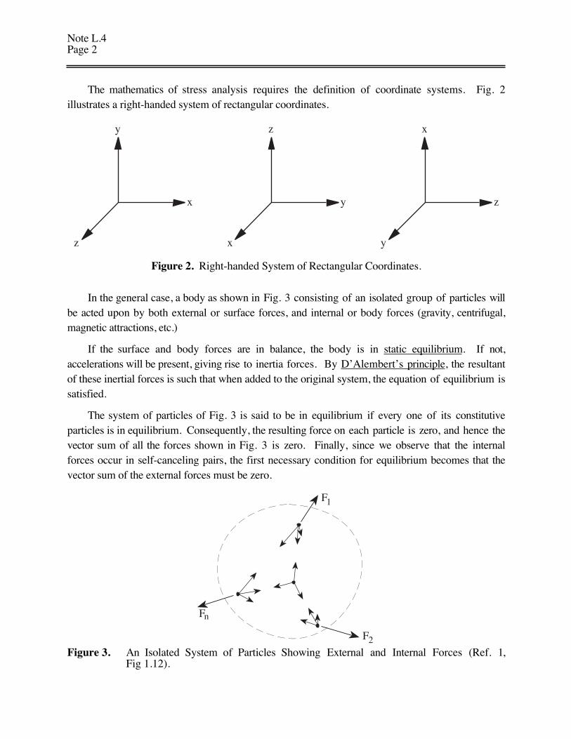
The mathematics of stress analysis requires the definition of coordinate systems. Fig. 2illustrates a right-handed system of rectangular coordinates.

y

x

z

z

y

x

x

z

y

Figure 2. Right-handed System of Rectangular Coordinates.

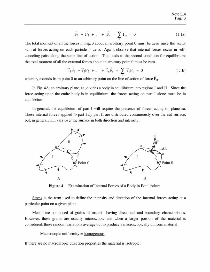
In the general case, a body as shown in Fig. 3 consisting of an isolated group of particles willbe acted upon by both external or surface forces, and internal or body forces (gravity, centrifugal,magnetic attractions, etc.)

If the surface and body forces are in balance, the body is in static equilibrium. If not,accelerations will be present, giving rise to inertia forces. By D’Alembert’s principle, the resultantof these inertial forces is such that when added to the original system, the equation of equilibrium issatisfied.

The system of particles of Fig. 3 is said to be in equilibrium if every one of its constitutiveparticles is in equilibrium. Consequently, the resulting force on each particle is zero, and hence thevector sum of all the forces shown in Fig. 3 is zero. Finally, since we observe that the internalforces occur in self-canceling pairs, the first necessary condition for equilibrium becomes that thevector sum of the external forces must be zero.

F

F

F

n

1

2Figure 3. An Isolated System of Particles Showing External and Internal Forces (Ref. 1,

Fig 1.12).

Note L.4Page 3

F1 + F2 + ... + Fn = Fn∑n

= 0 (1.1a)

The total moment of all the forces in Fig. 3 about an arbitrary point 0 must be zero since the vector

sum of forces acting on each particle is zero. Again, observe that internal forces occur in self-

canceling pairs along the same line of action. This leads to the second condition for equilibrium:

the total moment of all the external forces about an arbitrary point 0 must be zero.

r1F1 + r2F2 + ... + rnFn = rnFn∑n

= 0 (1.1b)

where rn extends from point 0 to an arbitrary point on the line of action of force Fn.

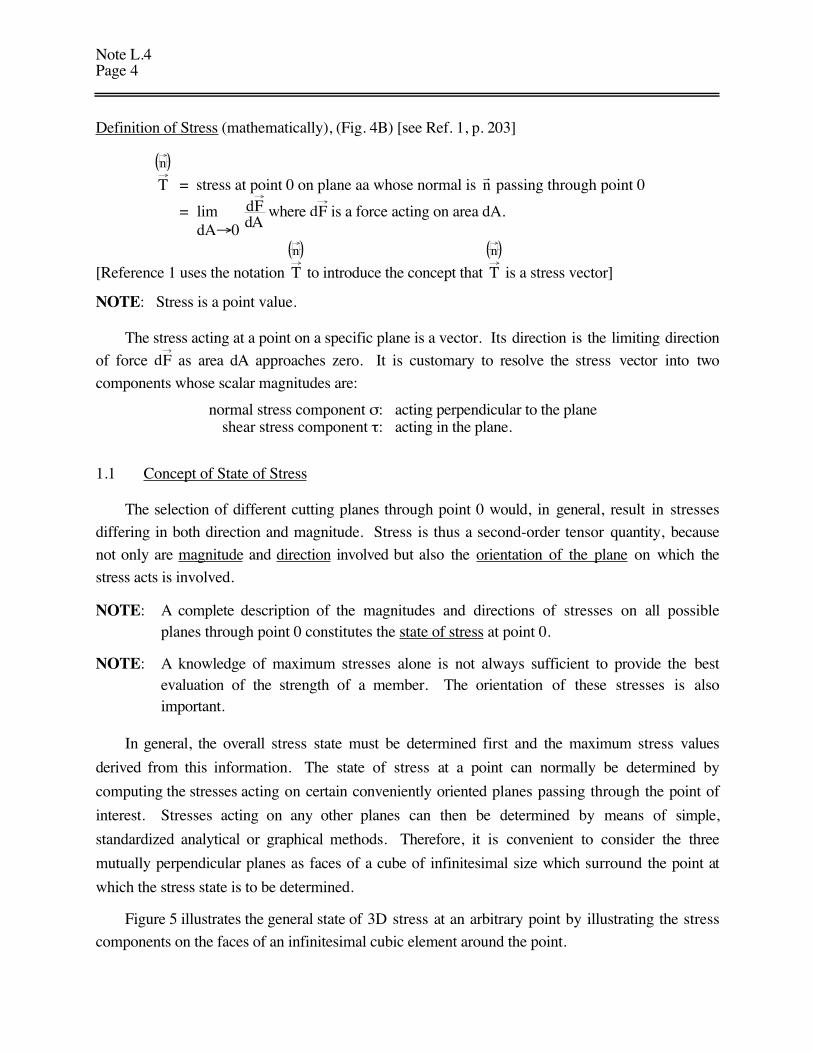
In Fig. 4A, an arbitrary plane, aa, divides a body in equilibrium into regions I and II. Since the

force acting upon the entire body is in equilibrium, the forces acting on part I alone must be in

equilibrium.

In general, the equilibrium of part I will require the presence of forces acting on plane aa.

These internal forces applied to part I by part II are distributed continuously over the cut surface,

but, in general, will vary over the surface in both direction and intensity.

dF

I

II

I

a

adA

A B

a

a

Point 0 Point 0

n

Figure 4. Examination of Internal Forces of a Body in Equilibrium.

Stress is the term used to define the intensity and direction of the internal forces acting at a

particular point on a given plane.

Metals are composed of grains of material having directional and boundary characteristics.

However, these grains are usually microscopic and when a larger portion of the material is

considered, these random variations average out to produce a macroscopically uniform material.

Macroscopic uniformity = homogenous,

If there are no macroscopic direction properties the material is isotropic.

Note L.4Page 4

Definition of Stress (mathematically), (Fig. 4B) [see Ref. 1, p. 203]

n

T = stress at point 0 on plane aa whose normal is rn passing through point 0

= lim dA→0

dFdA

where dF is a force acting on area dA.

[Reference 1 uses the notation

n

T to introduce the concept that

n

T is a stress vector]

NOTE: Stress is a point value.

The stress acting at a point on a specific plane is a vector. Its direction is the limiting direction

of force dF as area dA approaches zero. It is customary to resolve the stress vector into two

components whose scalar magnitudes are:

normal stress component σ: acting perpendicular to the planeshear stress component τ: acting in the plane.

1.1 Concept of State of Stress

The selection of different cutting planes through point 0 would, in general, result in stresses

differing in both direction and magnitude. Stress is thus a second-order tensor quantity, because

not only are magnitude and direction involved but also the orientation of the plane on which the

stress acts is involved.

NOTE: A complete description of the magnitudes and directions of stresses on all possibleplanes through point 0 constitutes the state of stress at point 0.

NOTE: A knowledge of maximum stresses alone is not always sufficient to provide the bestevaluation of the strength of a member. The orientation of these stresses is alsoimportant.

In general, the overall stress state must be determined first and the maximum stress values

derived from this information. The state of stress at a point can normally be determined by

computing the stresses acting on certain conveniently oriented planes passing through the point of

interest. Stresses acting on any other planes can then be determined by means of simple,

standardized analytical or graphical methods. Therefore, it is convenient to consider the three

mutually perpendicular planes as faces of a cube of infinitesimal size which surround the point at

which the stress state is to be determined.

Figure 5 illustrates the general state of 3D stress at an arbitrary point by illustrating the stress

components on the faces of an infinitesimal cubic element around the point.

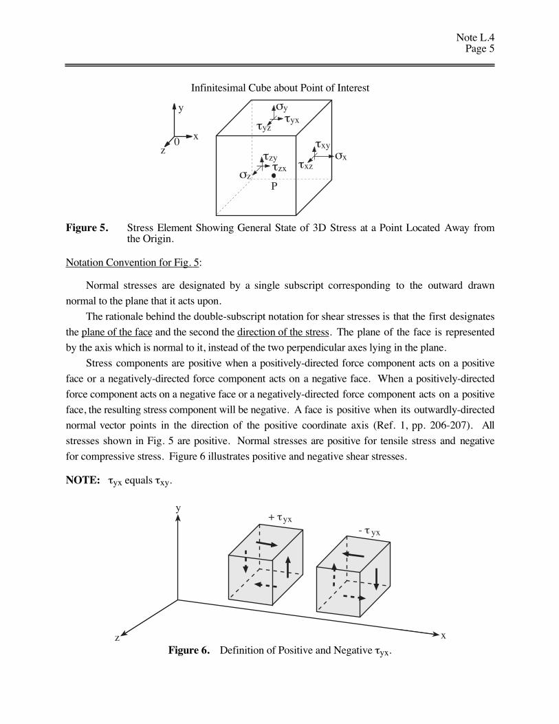
Note L.4Page 5

Infinitesimal Cube about Point of Interest

P

τzyτzxσz

σxτxy

τxz

σyτyxτyz

y

xz

0

Figure 5. Stress Element Showing General State of 3D Stress at a Point Located Away fromthe Origin.

Notation Convention for Fig. 5:

Normal stresses are designated by a single subscript corresponding to the outward drawn

normal to the plane that it acts upon.

The rationale behind the double-subscript notation for shear stresses is that the first designates

the plane of the face and the second the direction of the stress. The plane of the face is represented

by the axis which is normal to it, instead of the two perpendicular axes lying in the plane.

Stress components are positive when a positively-directed force component acts on a positive

face or a negatively-directed force component acts on a negative face. When a positively-directed

force component acts on a negative face or a negatively-directed force component acts on a positive

face, the resulting stress component will be negative. A face is positive when its outwardly-directed

normal vector points in the direction of the positive coordinate axis (Ref. 1, pp. 206-207). All

stresses shown in Fig. 5 are positive. Normal stresses are positive for tensile stress and negative

for compressive stress. Figure 6 illustrates positive and negative shear stresses.

NOTE: τyx equals τxy.

y

z x

+ τyx- τ yx

Figure 6. Definition of Positive and Negative τyx.

Note L.4Page 6

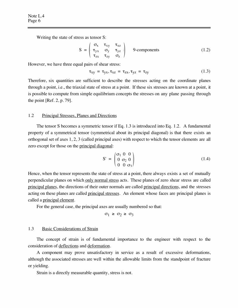
Writing the state of stress as tensor S:

S = σx τxy τxzτyx σy τyzτzx τzy σz

9-components (1.2)

However, we have three equal pairs of shear stress:

τxy = τyx, τxz = τzx, τyz = τzy (1.3)

Therefore, six quantities are sufficient to describe the stresses acting on the coordinate planes

through a point, i.e., the triaxial state of stress at a point. If these six stresses are known at a point, it

is possible to compute from simple equilibrium concepts the stresses on any plane passing through

the point [Ref. 2, p. 79].

1.2 Principal Stresses, Planes and Directions

The tensor S becomes a symmetric tensor if Eq. 1.3 is introduced into Eq. 1.2. A fundamental

property of a symmetrical tensor (symmetrical about its principal diagonal) is that there exists an

orthogonal set of axes 1, 2, 3 (called principal axes) with respect to which the tensor elements are all

zero except for those on the principal diagonal:

S' = σ1 0 00 σ2 00 0 σ3

(1.4)

Hence, when the tensor represents the state of stress at a point, there always exists a set of mutually

perpendicular planes on which only normal stress acts. These planes of zero shear stress are called

principal planes, the directions of their outer normals are called principal directions, and the stresses

acting on these planes are called principal stresses. An element whose faces are principal planes is

called a principal element.

For the general case, the principal axes are usually numbered so that:

σ1 ≥ σ2 ≥ σ3

1.3 Basic Considerations of Strain

The concept of strain is of fundamental importance to the engineer with respect to the

consideration of deflections and deformation.

A component may prove unsatisfactory in service as a result of excessive deformations,

although the associated stresses are well within the allowable limits from the standpoint of fracture

or yielding.

Strain is a directly measurable quantity, stress is not.

Note L.4Page 7

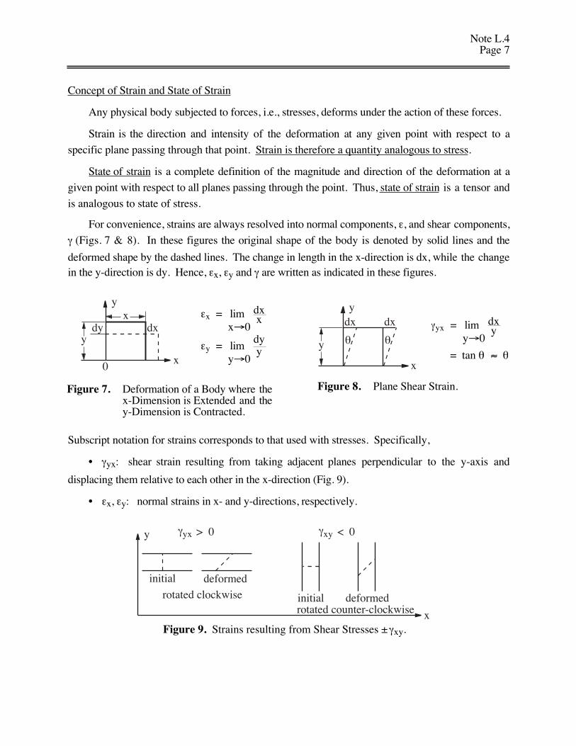
Concept of Strain and State of Strain

Any physical body subjected to forces, i.e., stresses, deforms under the action of these forces.

Strain is the direction and intensity of the deformation at any given point with respect to a

specific plane passing through that point. Strain is therefore a quantity analogous to stress.

State of strain is a complete definition of the magnitude and direction of the deformation at a

given point with respect to all planes passing through the point. Thus, state of strain is a tensor and

is analogous to state of stress.

For convenience, strains are always resolved into normal components, ε, and shear components,

γ (Figs. 7 & 8). In these figures the original shape of the body is denoted by solid lines and the

deformed shape by the dashed lines. The change in length in the x-direction is dx, while the changein the y-direction is dy. Hence, εx, εy and γ are written as indicated in these figures.

y

x

ydy dx

0

x εx = lim x→0

dxx

εy = lim y→0

dyy

Figure 7. Deformation of a Body where thex-Dimension is Extended and they-Dimension is Contracted.

y

x

y

dx

θ

dx

θγyx = lim

y→0 dxy

= tan θ ≈ θ

Figure 8. Plane Shear Strain.

Subscript notation for strains corresponds to that used with stresses. Specifically,

• γyx: shear strain resulting from taking adjacent planes perpendicular to the y-axis and

displacing them relative to each other in the x-direction (Fig. 9).

• εx, εy: normal strains in x- and y-directions, respectively.

y

x

initial deformed

rotated clockwise

γ yx > 0

initial deformedrotated counter-clockwise

γ xy < 0

Figure 9. Strains resulting from Shear Stresses ± γxy.

Note L.4Page 8

Sign conventions for strain also follow directly from those for stress: positive normal stressproduces positive normal strain and vice versa. In the above example (Fig. 7), εx > 0, whereasεy < 0. Adopting the positive clockwise convention for shear components, γxy < 0, γyx > 0. InFig. 8, the shear is γyx and the rotation is clockwise.

NOTE: Half of γxy, γxz, γyz is analogous to τxy , τxz and τyz , whereas εx is analogous to σx.

T =

εx 12

γxy12

γxz

12

γyx εy 12

γyz

12

γzx12

γzy εz

It may be helpful in appreciating the physical significance of the fact that τ is analogous to γ/2rather than with γ itself to consider Fig. 10. Here it is seen that each side of an element changes inslope by an angle γ/2.

γ2

γ2

Figure 10. State of Pure Shear Strain

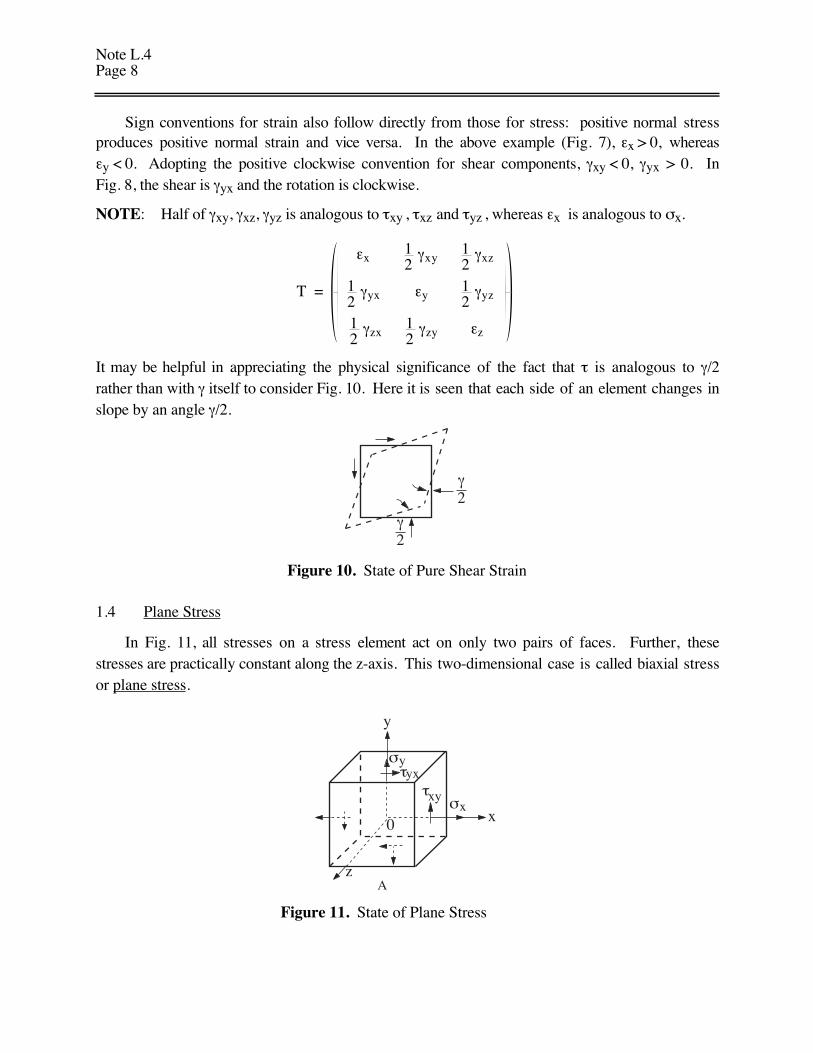
1.4 Plane Stress

In Fig. 11, all stresses on a stress element act on only two pairs of faces. Further, thesestresses are practically constant along the z-axis. This two-dimensional case is called biaxial stressor plane stress.

y

σyτyx

xσx

τxy

zA

0

Figure 11. State of Plane Stress

Note L.4Page 9

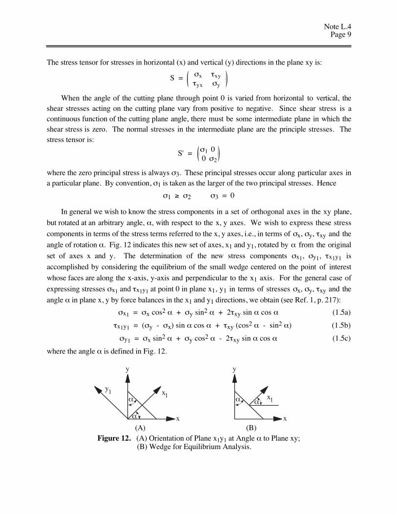
The stress tensor for stresses in horizontal (x) and vertical (y) directions in the plane xy is:

S = σx τxyτyx σy

When the angle of the cutting plane through point 0 is varied from horizontal to vertical, theshear stresses acting on the cutting plane vary from positive to negative. Since shear stress is acontinuous function of the cutting plane angle, there must be some intermediate plane in which theshear stress is zero. The normal stresses in the intermediate plane are the principle stresses. Thestress tensor is:

S' = σ1 00 σ2

where the zero principal stress is always σ3. These principal stresses occur along particular axes ina particular plane. By convention, σ1 is taken as the larger of the two principal stresses. Hence

σ1 ≥ σ2 σ3 = 0

In general we wish to know the stress components in a set of orthogonal axes in the xy plane,

but rotated at an arbitrary angle, α, with respect to the x, y axes. We wish to express these stress

components in terms of the stress terms referred to the x, y axes, i.e., in terms of σx, σy, τxy and the

angle of rotation α. Fig. 12 indicates this new set of axes, x1 and y1, rotated by α from the original

set of axes x and y. The determination of the new stress components σx1, σy1, τx1y1 is

accomplished by considering the equilibrium of the small wedge centered on the point of interest

whose faces are along the x-axis, y-axis and perpendicular to the x1 axis. For the general case of

expressing stresses σx1 and τx1y1 at point 0 in plane x1, y1 in terms of stresses σx, σy, τxy and the

angle α in plane x, y by force balances in the x1 and y1 directions, we obtain (see Ref. 1, p. 217):

σx1 = σx cos2 α + σy sin2 α + 2τxy sin α cos α (1.5a)

τx1y1 = (σy - σx) sin α cos α + τxy (cos2 α - sin2 α) (1.5b)

σy1 = σx sin2 α + σy cos2 α - 2τxy sin α cos α (1.5c)

where the angle α is defined in Fig. 12.

y

x

y x11α

α

y

x

x1α α

(A) (B)Figure 12. (A) Orientation of Plane x1y1 at Angle α to Plane xy;

(B) Wedge for Equilibrium Analysis.

Note L.4Page 10

These are the transformation equations of stress for plane stress. Their significance is that

stress components σx1, σy1 and τx1y1 at point 0 in a plane at an arbitrary angle α to the plane xy are

uniquely determined by the stress components σx, σy and τxy at point 0.

Eq. 1.5 is commonly written in terms of 2α. Using the identities:

sin2α = 1 - cos 2α

2 ; cos2α =

1 + cos 2α2

; 2 sin α cos α = sin 2α

we get

σx1 = σx + σy

2 +

σx - σy

2 cos 2α + τxy sin 2α (1.6a)

τx1y1 = - σx - σy

2 sin 2α + τxy cos 2α (1.6b)

σy1 = σx + σy

2 -

σx - σy

2 cos 2α - τxy sin 2α (1.6c)*

The orientation of the principal planes, in this two dimensional system is found by equating τx1y1 to

zero and solving for the angle α.

1.5 Mohr's Circle

Equations 1.6a,b,c, taken together, can be represented by a circle, called Mohr’s circle of stress.

To illustrate the representation of these relations, eliminate the function of the angle 2α from

Eq. 1.6a and 1.6b by squaring both sides of both equations and adding them. Before Eq. 1.6a is

squared, the term (σx + σy)/2 is transposed to the left side. The overall result is (where plane y1x1

is an arbitrarily located plane, so that σx1 is now written as σ and τx1y1 as τ):

[σ - 1/2 (σx + σy)]2 + τ2 = 1/4 (σx - σy)2 + τxy2 (1.7)

Now construct Mohr’s circle on the σ and τ plane. The principal stresses are those on the σ-axis

when τ = 0. Hence, Eq. 1.7 yields the principal normal stresses σ1 and σ2 as:

σ1,2 = σx + σy

2 ± τxy

2 + σx - σy

2

2(1.8)

center of circle radius

The maximum shear stress is the radius of the circle and occurs in the plane represented by a

vertical orientation of the radius.

* σy1 can also be obtained from σx1 by substituting α + 90˚ for α.

Note L.4Page 11

τmax = ± τxy2 +

σx - σy

2

2 = 1

2 σ1 - σ2 (1.9)

The angle between the principal axes x1y1 and the arbitrary axis, xy can be determined from

Eq. 1.6b by taking x1y1 as principal axes. Hence, from Eq. 1.6b with τx1y1 = 0 we obtain:

2α = tan-1 2τxy

σx - σy(1.10)

From our wedge we know an arbitrary plane is located an angle α from the general x-, y-axis set

and α ranges from zero to 180˚. Hence, for the circle with its 360˚ range of rotation, planes

separated by α in the wedge are separated by 2α on Mohr’s circle. Taking the separation between

the principal axis and the x-axis where the shear stress is τxy, we see that Fig. 13A also illustrates

the relation of Eq. 1.10. Hence, Mohr’s circle is constructed as illustrated in Fig. 13A.

σ

τ

α− σ

σx + σy

2

σx - σy

2

2α2 1

(σ , 0)2 (σ , 0)1(σ , τ )x xy

(σ , τ )y yx y

x

τxy2 +

σx - σy

2

2

-

-

+

+locus of yxτ locus of xyτ

A B

Figure 13. (A) Mohr’s Circle of Stress; (B) Shear Stress Sign Convection for Mohr’s Circle.*

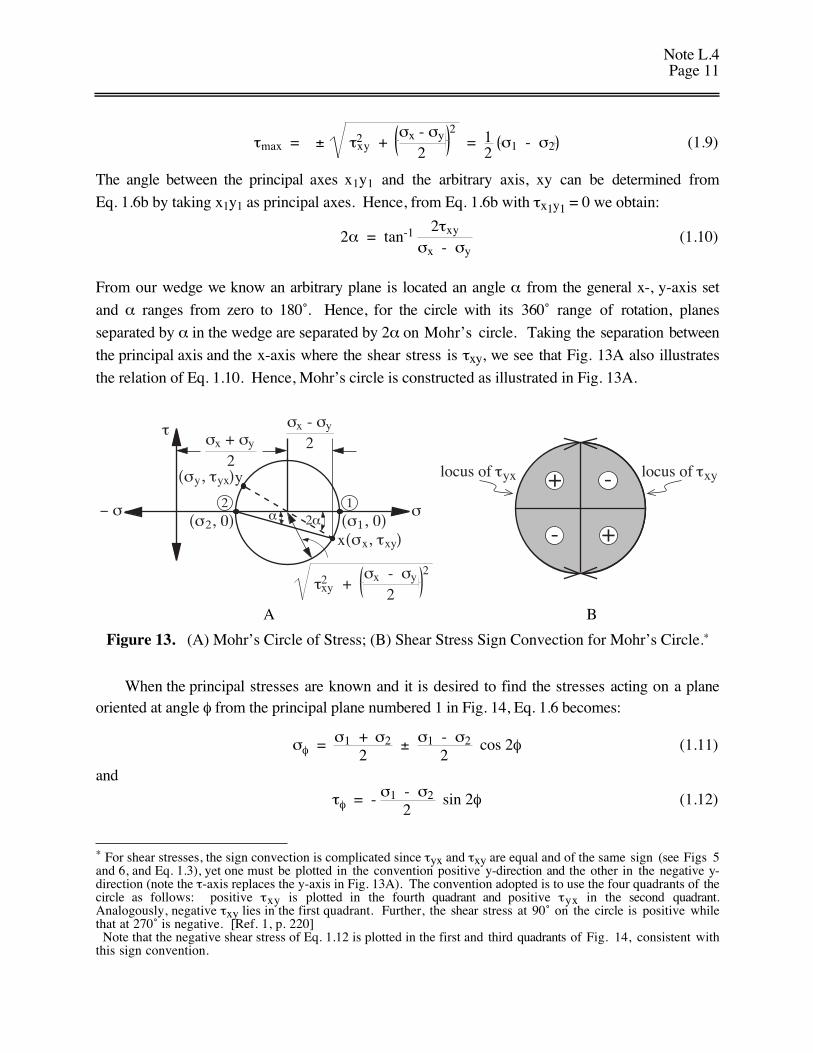
When the principal stresses are known and it is desired to find the stresses acting on a planeoriented at angle φ from the principal plane numbered 1 in Fig. 14, Eq. 1.6 becomes:

σφ = σ1 + σ22

± σ1 - σ22

cos 2φ (1.11)

and

τφ = - σ1 - σ22

sin 2φ (1.12)

* For shear stresses, the sign convection is complicated since τyx and τxy are equal and of the same sign (see Figs 5and 6, and Eq. 1.3), yet one must be plotted in the convention positive y-direction and the other in the negative y-direction (note the τ-axis replaces the y-axis in Fig. 13A). The convention adopted is to use the four quadrants of thecircle as follows: positive τxy is plotted in the fourth quadrant and positive τyx in the second quadrant.Analogously, negative τxy lies in the first quadrant. Further, the shear stress at 90˚ on the circle is positive whilethat at 270˚ is negative. [Ref. 1, p. 220] Note that the negative shear stress of Eq. 1.12 is plotted in the first and third quadrants of Fig. 14, consistent withthis sign convention.

Note L.4Page 12

σ

τ

σ

2φ2 1

1

σ1 + σ22

σ1 - σ22

cos 2φ

σ2

σ1 - σ22

sin 2φ

Figure 14. Mohr’s Circle Representation of Eqs. 1.11 & 1.12.

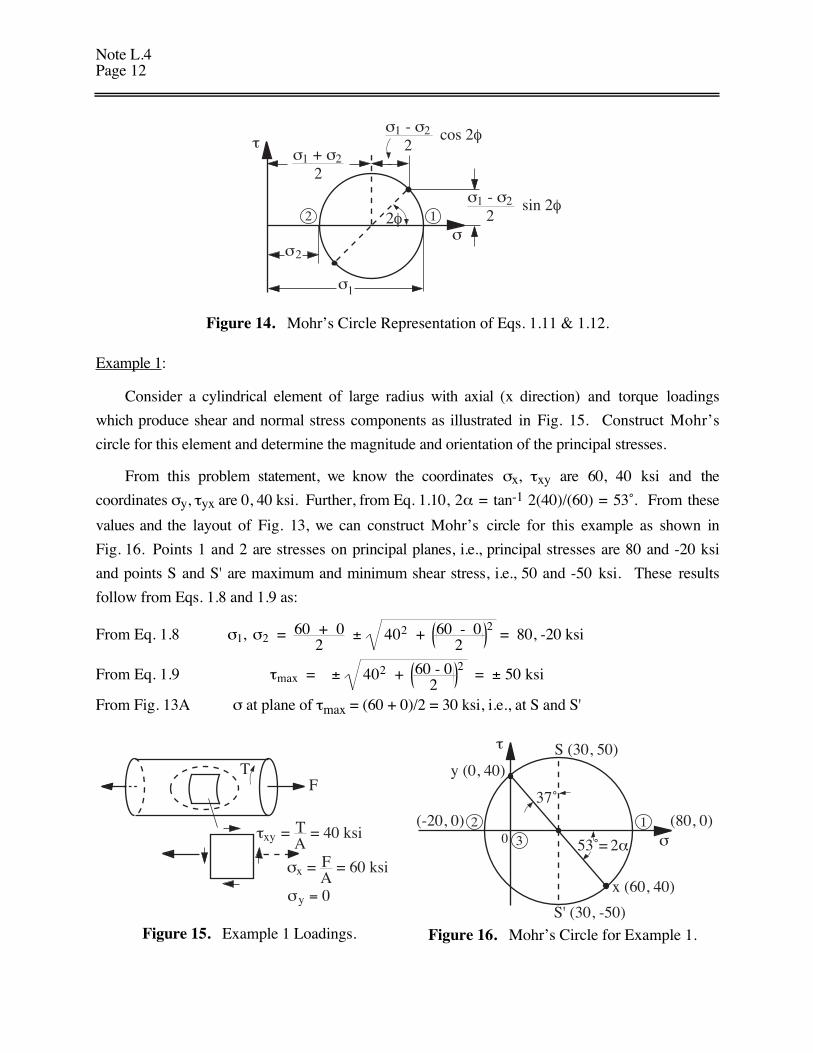
Example 1:

Consider a cylindrical element of large radius with axial (x direction) and torque loadings

which produce shear and normal stress components as illustrated in Fig. 15. Construct Mohr’s

circle for this element and determine the magnitude and orientation of the principal stresses.

From this problem statement, we know the coordinates σx, τxy are 60, 40 ksi and the

coordinates σy, τyx are 0, 40 ksi. Further, from Eq. 1.10, 2α = tan-1 2(40)/(60) = 53˚. From these

values and the layout of Fig. 13, we can construct Mohr’s circle for this example as shown in

Fig. 16. Points 1 and 2 are stresses on principal planes, i.e., principal stresses are 80 and -20 ksi

and points S and S' are maximum and minimum shear stress, i.e., 50 and -50 ksi. These results

follow from Eqs. 1.8 and 1.9 as:

From Eq. 1.8 σ1, σ2 = 60 + 02

± 402 + 60 - 02

2 = 80, -20 ksi

From Eq. 1.9 τmax = ± 402 + 60 - 02

2 = ± 50 ksi

From Fig. 13A σ at plane of τmax = (60 + 0)/2 = 30 ksi, i.e., at S and S'

σ = 0y

TF

τxy = TA

= 40 ksi

σx = FA

= 60 ksi

Figure 15. Example 1 Loadings.

σ

τ

37˚

2 1

53˚= 2α30(-20, 0)

y (0, 40)S (30, 50)

S' (30, -50)

(80, 0)

x (60, 40)

Figure 16. Mohr’s Circle for Example 1.

Note L.4Page 13

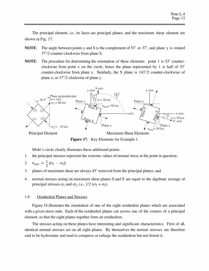
The principal element, i.e., its faces are principal planes, and the maximum shear element are

shown in Fig. 17.

NOTE: The angle between points y and S is the complement of 53˚ or 37 ,̊ and plane y is rotated37˚/2 counter-clockwise from plane S.

NOTE: The procedure for determining the orientation of these elements: point 1 is 53˚ counter-clockwise from point x on the circle; hence the plane represented by 1 is half of 53˚counter-clockwise from plane x. Similarly, the S plane is 143˚/2 counter-clockwise ofplane x, or 37˚/2 clockwise of plane y.

26.5˚

(2)

(2)

(1)

(1)

Plane perpendicularto x axisσ1 = 80 ksi

σ2 = - 20 ksi

Plane y σ = 30 ksi

Plane x

Plane S

Plane S

τmax= 50 ksi

143˚2

y axisS axis

x axis

37˚2

y axis

x axis

Plan

e S′

37˚2 σ = 30 ksi

S′ axis

Plan

e S′

Plane y

Plane xτmax= 50 ksi

Principal Element Maximum Shear Elements

Figure 17. Key Elements for Example 1.

Mohr’s circle clearly illustrates these additional points:

1. the principal stresses represent the extreme values of normal stress at the point in question;

2. τmax = 12

σ1 - σ2 ;

3. planes of maximum shear are always 45˚ removed from the principal planes; and

4. normal stresses acting on maximum shear planes S and S' are equal to the algebraic average ofprincipal stresses σ1 and σ2, i.e., 1/2 (σ1 + σ2).

1.6 Octahedral Planes and Stresses

Figure 18 illustrates the orientation of one of the eight octahedral planes which are associated

with a given stress state. Each of the octahedral planes cut across one of the corners of a principal

element, so that the eight planes together form an octahedron.

The stresses acting on these planes have interesting and significant characteristics. First of all,

identical normal stresses act on all eight planes. By themselves the normal stresses are therefore

said to be hydrostatic and tend to compress or enlarge the octahedron but not distort it.

Note L.4Page 14

σoct = σ1 + σ2 + σ33

(1.13a)

Shear stresses are also identical. These distort the octahedron without changing its volume.

Although the octahedral shear stress is smaller than the highest principal shear stress, it constitutes

a single value that is influenced by all three principal shear stresses. Thus, it is important as a

criterion for predicting yielding of a stressed material.

τoct = 13

σ1 - σ22 + σ2 - σ3

2 + σ3 - σ12 1/2 (1.13b)

In cases in which σx, σy, σz, τxy, τxz and τyz are known:

σoct = σx + σy + σz

3(1.14a)

τoct = 13

σx - σy2 + σy - σz

2 + σz - σx2 + 6 τxy

2 + τxz2 + τyz

2 1/2 (1.14b)

σ1

σ2

σ3

σoct

τ oct

Figure 18. Octahedral Planes Associated with a Given Stress State.

1.7 Principal Strains and Planes

Having observed the correspondence between strain and stress, it is evident that with suitable

axis transformation one obtains an expression for the strain tensor T ' which is identical to that of

stress tensor S' except that the terms in the principal diagonal are ε1, ε2, ε3. Hence, recalling from

Section 1.3 that γ/2 corresponds to τ, strain relations analogous to Eqs. 1.8, 1.9 and 1.10 can be

written as follows:

ε1, ε2 = εx + εy

2 ± 1

2 γxy

2 +

εx - εy

2

2(1.15)

γmax = ± 2 12

γxy2 +

εx - εy

2

2(1.16)

2α = tan-1 γxy

εx - εy(1.17)

Note L.4Page 15

Conclusion

The preceding sections dealt separately with the concepts of stress and strain at a point. These

considerations involving stresses and strains separately are general in character and applicable to

bodies composed of any continuous distribution of matter.

NOTE: No material properties were involved in the relationships, hence they are applicable to

water, oil, as well as materials like steel and aluminum.

Note L.4Page 16

intentionally left blank

Note L.4Page 17

2. ELASTIC STRESS-STRAIN RELATIONS

The relationships between these quantities are of direct importance to the engineer concerned

with design and stress analysis. Generally two principal types of problems exist:

1. Determination of the stress state at a point from a known strain state—the problem

encountered when stresses are to be computed from experimentally determined strains.

2. Determination of the state of strain at a point from a known stress state—the problem

commonly encountered in design, where a part is assured to carry certain loads, and strains

must be computed with regard to critical clearances and stiffnesses.

We limit ourselves to solids loaded in the elastic range. Furthermore, we shall consider only

materials which are isotropic, i.e., materials having the same elastic properties in all directions.

Most engineering materials can be considered as isotropic. Notable exceptions are wood and

reinforced concrete.

2.1 Generalized Hooke’s Law

Let us consider the various components of stress one at a time and add all their strain effects.

For a uni-axial normal stress in the x direction, σx, the resulting normal strain is

εx = σxE

(2.1)

where E is Young’s modulus or the modulus of elasticity.

Additionally this stress produces lateral contraction, i.e., εy and εz, which is a fixed fraction of

the longitudinal strain, i.e.,

εy = εz = - νεx = - ν σxE

. (2.2)

This fixed fraction is called Poisson’s ratio, ν. Analogous results are obtained from strains due to

σy and σz.

The shear-stress components produce only their corresponding shear-strain components that

are expressed as:

γzx = τzxG

, γxy = τxy

G , γyz =

τyz

G(2.3a,b,c)

where the constant of proportionality, G, is called the shear modulus.

Note L.4Page 18

For a linear-elastic isotropic material with all components of stress present:

εx = 1E

σx - ν σy + σz (2.4a)

εy = 1E

σy - ν σz + σx (2.4b)

εz = 1E

σz - ν σx + σy (2.4c)

γxy = τxy

G (2.5a) same as (2.3)

γyz = τyz

G (2.5b)

γzx = τzxG

(2.5c)

These equations are the generalized Hooke’s law.

It can also be shown (Ref 1, p. 285) that for an isotropic materials, the properties G, E and ν

are related as:

G = E2 (1 + ν)

. (2.6)

Hence,

γxy = 2 (1 + ν)

E τxy (2.7a)

γyz = 2 (1 + ν)

E τyz (2.7b)

γzx = 2 (1 + ν)

E τzx . (2.7c)

Equations 2.4 and 2.5 may be solved to obtain stress components as a function of strains:

σx = E(1 + ν) (1 - 2ν)

1 - ν εx + ν εy + εz (2.8a)

σy = E(1 + ν) (1 - 2ν)

1 - ν εy + ν εz + εx (2.8b)

σz = E(1 + ν) (1 - 2ν)

1 - ν εz + ν εx + εy (2.8c)

τxy = E2 (1 + ν)

γxy = Gγxy (2.9a)

τyz = E2 (1 + ν)

γyz = Gγyz (2.9b)

τzx = E2 (1 + ν)

γzx = Gγzx . (2.9c)

Note L.4Page 19

For the first three relationships one may find:

σx = E(1 + ν)

εx + ν(1 - 2ν)

εx + εy + εz (2.10a)

σy = E(1 + ν)

εy + ν(1 - 2ν)

εx + εy + εz (2.10b)

σz = E(1 + ν)

εz + ν(1 - 2ν)

εx + εy + εz . (2.10c)

For special case in which the x, y, z axes coincide with principal axes 1, 2, 3, we can simplify the

strain set, Eqs. 2.4 and 2.5, and the stress set Eqs. 2.8 and 2.9, by virtue of all shear strains and

shear stresses being equal to zero.

ε1 = 1E

σ1 - ν σ2 + σ3 (2.11a)

ε2 = 1E

σ2 - ν σ3 + σ1 (2.11b)

ε3 = 1E

σ3 - ν σ1 + σ2 (2.11c)

σ1 = E(1 + ν) (1 - 2ν)

1 - ν ε1 + ν ε2 + ε3 (2.12a)

σ2 = E(1 + ν) (1 - 2ν)

1 - ν ε2 + ν ε3 + ε1 (2.12b)

σ3 = E(1 + ν) (1 - 2ν)

1 - ν ε3 + ν ε1 + ε2 . (2.12c)

For biaxial-stress state, one of the principal stresses (say σ3) = 0, Eqs. 2.11a,b,c become:

ε1 = 1E

σ1 - νσ2 (2.13a)

ε2 = 1E

σ2 - νσ1 (2.13b)

ε3 = - νE

σ1 + σ2 . (2.13c)

In simplifying Eqs. 2.12a,b,c for the case of σ3 = 0, we note from Eq. 2.12c that for σ3 to be zero,

ε3 = - ν1 - ν

ε1 + ε2 . (2.14)

Substituting this expression into the first two of Eqs. 2.12a,b,c gives:

σ1 = E1 - ν2

ε1 + νε2 (2.15a)

σ2 = E1 - ν2

ε2 + νε1 (2.15b)

σ3 = 0 . (2.15c)

Note L.4Page 20

In case of uniaxial stress Eqs. 2.13 and 2.15 must, of course reduce to:

ε1 = 1E

σ1 (2.16a)

ε2 = ε3 = - νE

σ1 (2.16b)

σ1 = Eε1 (2.17a)

σ2 = σ3 = 0 . (2.17b)

2.2 Modulus of Volume Expansion (Bulk Modulus)

k may be defined as the ratio between hydrostatic stress (in which σ1 = σ2 = σ3) and

volumetric strain (change in volume divided by initial volume), i.e.,

k = σ/(∆V/V). (2.18)

NOTE: Hydrostatic compressive stress exists within the fluid of a pressurized hydraulic cylinder,

in a rock at the bottom of the ocean or far under the earth’s surface, etc.

Hydrostatic tension can be created at the interior of a solid sphere by the sudden

application of uniform heat to the surface, the expansion of the surface layer subjecting

the interior material to triaxial tension. For σ1 = σ2 = σ3 = σ, Eqs. 2.11a,b,c show that:

ε1 = ε2 = ε3 = ε = σE

1 - 2ν .

This state of uniform triaxial strain is characterized by the absence of shearing deformation; an

elemental cube, for example, would change in size but remain a cube. The size of an elemental cube

initially of unit dimension would change from 13 to (1 + ε)3 or to 1 + 3ε + 3ε2 + ε3. If we

consider normal structural materials, ε is a quantity sufficiently small, so that ε2 and ε3 are

completely negligible, and the volumetric change is from 1 to 1 + 3ε. The volumetric strain, ∆V/V,

is thus equal to 3ε or to:

∆VV

= 3ε = 3σ (1 - 2ν)

E . (2.19)

Hence,k ≡ σ

3ε = E

3 (1 - 2ν) . (2.20)

Now ν ≤ 0.5, so that k cannot become negative. A simple physical model of a representative

atomic crystalline structure gives:

ν = 1/3 , (2.21)so that

k = E . (2.22)

Note L.4Page 21

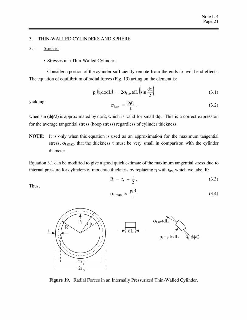
3. THIN-WALLED CYLINDERS AND SPHERE

3.1 Stresses

• Stresses in a Thin-Walled Cylinder:

Consider a portion of the cylinder sufficiently remote from the ends to avoid end effects.

The equation of equilibrium of radial forces (Fig. 19) acting on the element is:

pi ridφdL = 2σt,avtdL sin dφ2

(3.1)

yieldingσt,av =

piri

t . (3.2)

when sin (dφ/2) is approximated by dφ/2, which is valid for small dφ. This is a correct expression

for the average tangential stress (hoop stress) regardless of cylinder thickness.

NOTE: It is only when this equation is used as an approximation for the maximum tangential

stress, σt,max, that the thickness t must be very small in comparison with the cylinder

diameter.

Equation 3.1 can be modified to give a good quick estimate of the maximum tangential stress due to

internal pressure for cylinders of moderate thickness by replacing ri with rav, which we label R:

R = ri + t2

. (3.3)

Thus,

σt,max ≈ piR

t(3.4)

p

t

2ri2ro

i dφR

dLdφ/2p r dφdLii

σ tdLt,av

Figure 19. Radial Forces in an Internally Pressurized Thin-Walled Cylinder.

Note L.4Page 22

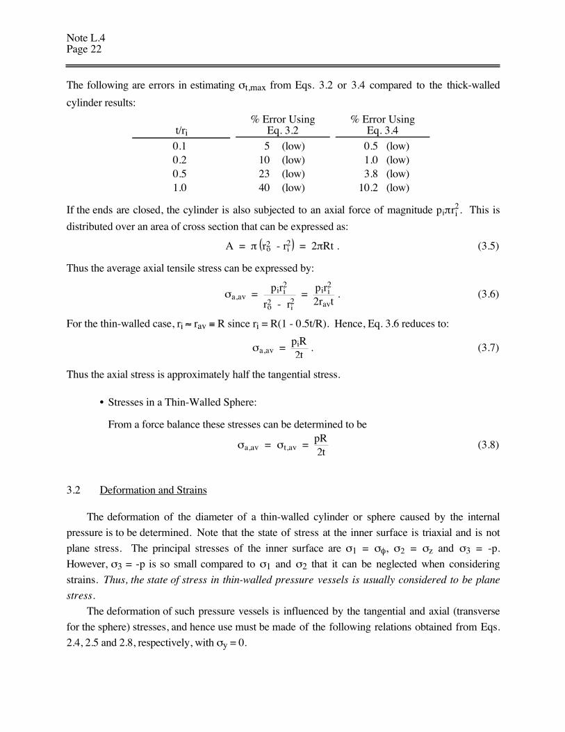
The following are errors in estimating σt,max from Eqs. 3.2 or 3.4 compared to the thick-walled

cylinder results:

t/ri

% Error UsingEq. 3.2

% Error UsingEq. 3.4

0.1 5 (low) 0.5 (low)0.2 10 (low) 1.0 (low)0.5 23 (low) 3.8 (low)1.0 40 (low) 10.2 (low)

If the ends are closed, the cylinder is also subjected to an axial force of magnitude piπri2. This is

distributed over an area of cross section that can be expressed as:

A = π ro2 - ri2 = 2πRt . (3.5)

Thus the average axial tensile stress can be expressed by:

σa,av = piri

2

ro2 - ri2 =

piri2

2ravt . (3.6)

For the thin-walled case, ri ≈ rav ≡ R since ri = R(1 - 0.5t/R). Hence, Eq. 3.6 reduces to:

σa,av = piR2t

. (3.7)

Thus the axial stress is approximately half the tangential stress.

• Stresses in a Thin-Walled Sphere:

From a force balance these stresses can be determined to be

σa,av = σt,av = pR2t

(3.8)

3.2 Deformation and Strains

The deformation of the diameter of a thin-walled cylinder or sphere caused by the internal

pressure is to be determined. Note that the state of stress at the inner surface is triaxial and is not

plane stress. The principal stresses of the inner surface are σ1 = σφ, σ2 = σz and σ3 = -p.

However, σ3 = -p is so small compared to σ1 and σ2 that it can be neglected when considering

strains. Thus, the state of stress in thin-walled pressure vessels is usually considered to be plane

stress.

The deformation of such pressure vessels is influenced by the tangential and axial (transverse

for the sphere) stresses, and hence use must be made of the following relations obtained from Eqs.

2.4, 2.5 and 2.8, respectively, with σy = 0.

Note L.4Page 23

εx = σxE

- νσzE

(3.9a)

εy = - νE

σx + σz (3.9b)

εz = σzE

- νσxE

(3.9c)

γ = τxy

G(3.9d)

σx = E1 - ν2

εx + νεz (3.10a)

σz = E1 - ν2

εz + νεx (3.10b)

to express Hooke’s law for plane stress. Equations 3.10a,b are obtained from Eqs. 2.8a and 2.8c

upon inspection of εy evaluated from Eq. 2.8b with σy taken as zero.

Let σφ, σz, εφ and εz represent the tangential and axial stress and strain, respectively, in the wall.

The substitution of these symbols in Eqs. 3.9a,b,c, i.e., x ≡ φ and z = z, gives:

εφ = σφ

E - ν σz

E(3.11)

εz = σzE

- ν σφ

E . (3.12)

• Closed-End Cylinder:

For the strains in the closed-end cylinder, the values of σφ and σz as derived in Eqs. 3.4

and 3.8, respectively, are substituted into Eqs. 3.11 and 3.12 to give:

εφ = 1E

pRt

- ν pR2t

= pR2Et

(2 - ν) (3.13)

εz = 1E

pR2t

- ν pRt

= pR2Et

(1 - 2ν) . (3.14)

Let the change in length of radius R be ∆r when the internal pressure is applied. Then the change in

length of the circumference is 2π∆r. But the circumferential strain, εφ, is, by definition, given by the

following equation:

εφ = 2π∆r2πR

= ∆rR

. (3.15)

By combining Eqs. 3.15 and 3.13 we get:

∆r = pR2

2Et (2 - ν) . (3.16)

Note L.4Page 24

The change in length, ∆l, for a closed-end cylinder is equal to:

∆l = εzl (3.17)

or∆l =

pRl

2Et (1 - 2ν) (3.18)

• Sphere:

σz = σφ = pR2t

(3.19)

Thus, from Eq. 3.11:

εφ = 1E

pR2t

- ν pR2t

= pR2Et

(1 - ν) . (3.20)

By combining Eq. 3.20 with Eq. 3.15, we obtain:

∆r = pR2

2Et (1 - ν) . (3.21)

3.3 End Effects for the Closed-End Cylinder

Figure 20 illustrates a cylinder closed by thin-walled hemispherical shells. They are joined

together at AA and BB by rivets or welds. The dashed lines show the displacements due to internal

pressure, p. These displacements are given by Eqs. 3.16 and 3.21 as:

∆Rc = pR2

2Et (2 - ν) (3.22a)

∆Rs = pR2

2Et (1 - ν) (3.22b)

The value of ∆Rc is more than twice that of ∆Rs for the same thickness, t, and as a result the

deformed cylinder and hemisphere do not match boundaries. To match boundaries, rather large

shearing forces, V, and moments, M, must develop at the joints as Fig. 20 depicts (only those on the

cylinder are shown; equal but opposite shears and moments exist on the ends of the hemispheres).

This shear force is considerably minimized in most reactor pressure vessels by sizing the

hemisphere thickness much smaller than the cylinder thickness. For example, if the hemisphere

thickness is 120 mm and the cylinder thickness is 220 mm, for ν = 0.3, then the ratio ∆Rc to ∆Rs is

∆Rc

∆Rs

= tstc

2 - ν1 - ν

= 1.32

Note L.4Page 25

ΑV

ΒV

∆Rc

V

V

Α

Β

Rs

∆Rs

V ≡ Shearing Forces

Μ Μ

ΜΜ

Figure 20. Discontinuities in Strains for the Cylinder (∆Rc) and the Sphere (∆Rs).

The general solution of the discontinuity stresses induced by matching cylindrical and

hemisphere shapes is not covered in these notes. However, a fundamental input to this solution is

the matching of both displacements and deflections of the two cylinders of different wall

thicknesses at the plane they join. Thus, the relationship between load, stress, displacement and

deflection for cylinders and hemispheres are derived. These relations are presented in Tables 1

and 2, respectively.

Table 1. Relationship Between Load, Stresses, Displaced and Deflection for the Cylinder(equations cited are from Ref. 2)

Load

Stressesσt, σl, σr

σθ, σz, σr

Displacement

uo

Deflection

θo

ppRt

, pR2t

, - p2

pR2

2tE 2 - ν + ν t

R0

Mo

EdgeMomentper UnitPerimeterLength

EMo

2β2DR

± γ 6Mo

t2 , ± 6Mo

t2 , 0

(Eq. 7.3.22, (Eq. 7.3.21,p. 7.3-12) p. 7.3-11)

Note: uM

Doo=

2 2β ; so first term

= EuR

o .

Mo

2β2D

(Eq. 7.3.18, p. 7.3.7)

units F ⋅ L/L

1L2

FL2

L3 = L

- Mo

βD

(Eq. 7.3.19, p. 7.3.8)

dimensionless

Table 1 continued on next page

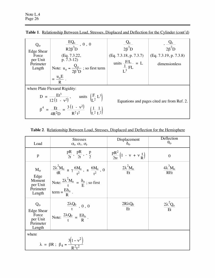
Note L.4Page 26

Table 1. Relationship Between Load, Stresses, Displaced and Deflection for the Cylinder (cont’d)

Qo

Edge ShearForce

per UnitPerimeterLength

EQo

R2β3D

, 0 , 0

(Eq. 7.3.22,p. 7.3-12)

Note: uQ

Doo=

2 3β ; so first term

= u ERo .

Qo

2β3D

(Eq. 7.3.18, p. 7.3.7)

units F/L1L3

FL = L

- Qo

2β2D

(Eq. 7.3.19, p. 7.3.8)

dimensionless

where Plate Flexural Rigidity:

D = Et3

12 1 - ν2 , units F

L2 L3

β4 = Et

4R2D =

3 1 - ν2

R2 t21L2

1L2

Equations and pages cited are from Ref. 2.

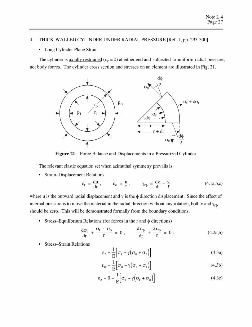
Table 2. Relationship Between Load, Stresses, Displaced and Deflection for the Hemisphere

LoadStressesσt, σl, σr

Displacementδo

Deflectionθo

ppR2t

, pR2t

, - p2

pR2

2tε 1 - ν + ν t

R 0

Mo

EdgeMomentper UnitPerimeterLength

2λ2Mo

tR ± γ 6Mo

t2 , ± 6Mo

t2 , 0

Note: 2λ2Mot

= δoE

; so first

term = EδoR

.

2λ2Mo

Et4λ

3Mo

REt

Qo

Edge ShearForce

per UnitPerimeterLength

2λQ0

t , 0 , 0

Note:

2λQ0

t = Eδo

R .

2RλQ0

Et2λ

2Qo

Et

where

λ = βR ; βν

4

2

2 2

3 1=

−( )R t

Note L.4Page 27

4. THICK-WALLED CYLINDER UNDER RADIAL PRESSURE [Ref. 1, pp. 293-300]

• Long Cylinder Plane Strain

The cylinder is axially restrained (εz = 0) at either end and subjected to uniform radial pressure,

not body forces. The cylinder cross section and stresses on an element are illustrated in Fig. 21.

pi ri

ropo

dφrσ

rr + dr

dφ2

φσ

φσdφ2

rσ + d rσ

Figure 21. Force Balance and Displacements in a Pressurized Cylinder.

The relevant elastic equation set when azimuthal symmetry prevails is

• Strain–Displacement Relations

εr = dudr

, εφ = ur , γrφ = dvdr

- vr (4.1a,b,c)

where u is the outward radial displacement and v is the φ direction displacement. Since the effect of

internal pressure is to move the material in the radial direction without any rotation, both v and γrφ

should be zero. This will be demonstrated formally from the boundary conditions.

• Stress–Equilibrium Relations (for forces in the r and φ directions)

dσrdr

+ σr - σφ

r = 0 , dτrφ

dr +

2τrφ

r = 0 . (4.2a,b)

• Stress–Strain Relations

ε σ γ σ σφr r zE= − +( )[ ]1

(4.3a)

ε σ γ σ σφ φ= − +( )[ ]1E z r (4.3b)

ε σ γ σ σφz z rE= = − +( )[ ]0

1(4.3c)

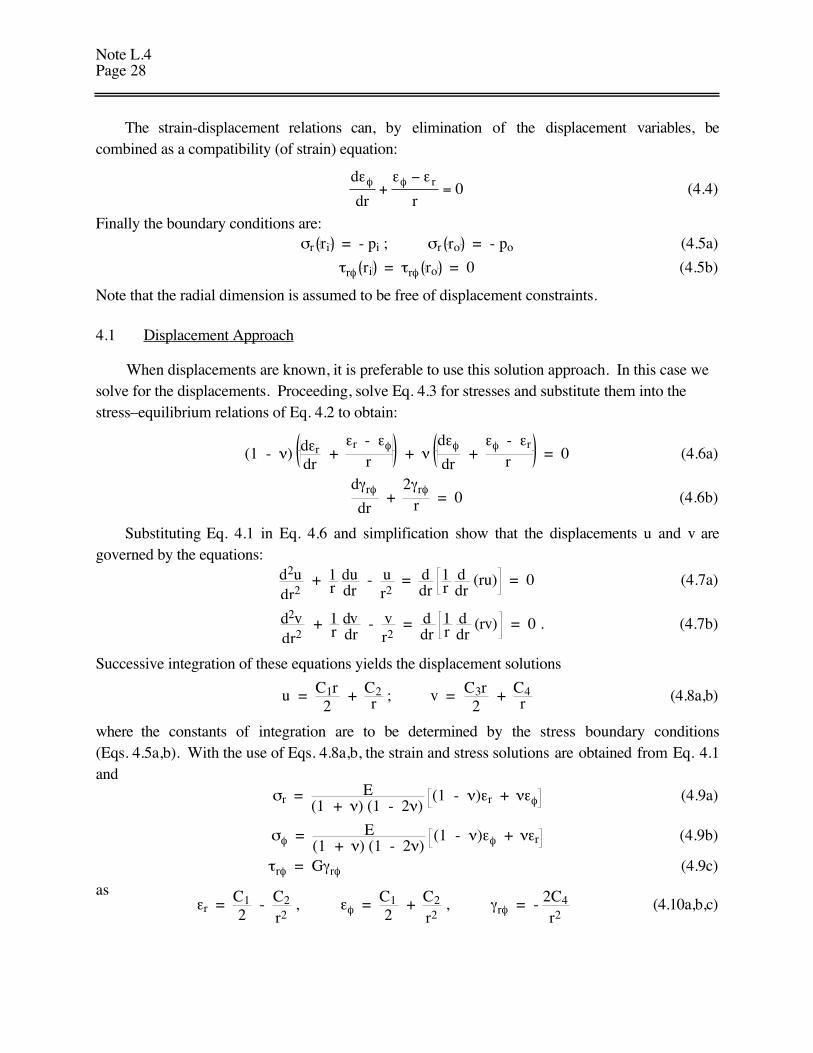
Note L.4Page 28

The strain-displacement relations can, by elimination of the displacement variables, becombined as a compatibility (of strain) equation:

d

dr rrε ε εφ φ+

−= 0 (4.4)

Finally the boundary conditions are:σr ri = - pi ; σr ro = - po (4.5a)

τrφ ri = τrφ ro = 0 (4.5b)

Note that the radial dimension is assumed to be free of displacement constraints.

4.1 Displacement Approach

When displacements are known, it is preferable to use this solution approach. In this case wesolve for the displacements. Proceeding, solve Eq. 4.3 for stresses and substitute them into thestress–equilibrium relations of Eq. 4.2 to obtain:

(1 - ν) dεrdr

+ εr - εφ

r + ν dεφ

dr +

εφ - εr

r = 0 (4.6a)

dγrφ

dr +

2γrφ

r = 0 (4.6b)

Substituting Eq. 4.1 in Eq. 4.6 and simplification show that the displacements u and v aregoverned by the equations:

d2udr2

+ 1r dudr

- ur2

= ddr

1r d

dr (ru) = 0 (4.7a)

d2vdr2

+ 1r dvdr

- vr2

= ddr

1r d

dr (rv) = 0 . (4.7b)

Successive integration of these equations yields the displacement solutions

u = C1r2

+ C2r ; v = C3r

2 + C4

r (4.8a,b)

where the constants of integration are to be determined by the stress boundary conditions(Eqs. 4.5a,b). With the use of Eqs. 4.8a,b, the strain and stress solutions are obtained from Eq. 4.1and

σr = E(1 + ν) (1 - 2ν)

(1 - ν)εr + νεφ (4.9a)

σφ = E(1 + ν) (1 - 2ν)

(1 - ν)εφ + νεr (4.9b)

τrφ = Gγrφ (4.9c)

asεr = C1

2 - C2

r2 , εφ = C1

2 + C2

r2 , γrφ = - 2C4

r2(4.10a,b,c)

Note L.4Page 29

σr = E(1 + ν) (1 - 2ν)

C12

- (1 - 2ν) C2

r2(4.11a)

σφ = E(1 + ν) (1 - 2ν)

C12

+ (1 - 2ν) C2

r2(4.11b)

σz = ν σr + σφ νEC1(1 + ν) (1 - 2ν)

(4.11c)

τrφ = - 2GC4

r2 . (4.11d)

By virtue of the boundary conditions, Eqs. 4.5a,b, the first and last of Eq. 4.11 yield thefollowing equations for the determination of the constants C1 and C2.

C12

- (1 - 2ν) C2

ri2

= - (1 + ν) (1 - 2ν)

E pi (4.12a)

C12

- (1 - 2ν) C2

ro2 = -

(1 + ν) (1 - 2ν)E

po (4.12b)

C4 = 0 (4.12c)

The solutions for C1 and C2 are

C12

= (1 + ν) (1 - 2ν) piri

2 - poro2

E ro2 - ri2

(4.13a)

C2 = (1 + ν) pi - po ri

2ro2

E ro2 - ri2

. (4.13b)

As to the constant C3, it remains undetermined. However, with C4 = 0, Eq. 4.8 shows that v = C3r/2which corresponds to a rigid-body rotation about the axis of the cylinder. Since this rotation doesnot contribute to the strains, C3 is taken as zero. Hence Eqs. 4.11a,b,c and Eq. 4.8a become:

σr = 1ro/ri

2 - 1 1 -

ro/ri2

r/ri2

pi - 1 - 1r/ri

2 ro

ri

2po (4.14a)

σφ = 1ro/ri

2 - 1 1 +

ro/ri2

r/ri2

pi - 1 + 1r/ri

2 ro

ri

2po (4.14b)

σz = 2νro/ri

2 - 1 pi -

rori

2po Plane Strain! (4.14c)

u = (1 + ν) r/ri ri

ro/ri2 - 1

(1 - 2ν) + ro/ri

2

r/ri2

pi

E - (1 - 2ν) + 1

r/ri2

rori

2 po

E(4.14d)

4.2 Stress Approach

In this case we solve directly for the stresses and apply the boundary conditions as before.Thus, re-expressing the stress-strain relations (Eq. 4.3) directly as strain when εz = 0 we get:

Note L.4Page 30

εr = 1 + νE

(1 - ν) σr - νσφ (4.15a)

εφ = 1 + νE

(1 - ν) σφ - νσr (4.15b)

γrφ = τrφ

G , (4.15c)

and then substituting them into Eq. 4.4 upon simplification yields

1 0−( ) − +−

=νσ

νσ σ σφ φd

drddr r

r r . (4.16)

By the first stress-equilibrium relation in Eq. 4.2, this equation is reduced to the simple form

ddr

σr + σφ = 0 . (4.17)

Integration of this equation and the second of Eq. 4.2 yields

σ σφr C+ = 1 ; τ φrC

r= 2

2 . (4.18a,b)

Substitution of the relation σφ = C1 - σr in Eq. 4.2, transposition, and integration yield

σr = C12

+ C3

r2 , (4.19)

where C1, C2 and C3 are constants of integration. Applying the boundary conditions we finally get

C1 = piri

2 - poro2

ro2 - ri2

, C2 = 0 , C3 = pi - po ri

2ro2

ro2 - ri2

. (4.20a,b,c)

With these values for the constants, Eqs. 4.18, 4.19 and the relation σz = ν(σr + σφ), the complete

stress solution is explicitly given. This solution can then be substituted in Eqs. 4.15a and 4.15b to

determine εr and εφ and, finally, u is determined by the relation u = rεφ.

NOTE: Since the prescribed boundary conditions of the problem are stresses, it is evident that the

stress approach in obtaining the solution involves simpler algebra than the displacement

approach.

Note L.4Page 31

5. THERMAL STRESS

Let us consider the additional stresses if the cylinder wall is subjected to a temperature gradient

due to an imposed internal wall temperature, T1, and an external wall temperature, To. For this case

the following stresses and stress gradients are zero,

τrφ ; τzφ and ∂σφ

∂φ = 0 (5.1a,b,c)

τrz = 0 and ∂σz

∂z = 0 (5.1d, e)

NOTE: All boundary planes are planes of principal stress.

For this case the governing equations become:

• Equilibrium∂σr

∂r -

σφ - σr

r = 0 (5.2)

• The strain equation can be applied to get

Eεr = E ∂u

∂r = σr - νσφ - νσz + EαT (5.3a)

Eεφ = E ur = σφ - νσr - νσz + EαT (5.3b)

Eεz = E ∂w

∂z = σz - νσr - νσφ + EαT (5.3c)

• Compatibility∂

∂r u

r = 1r ∂u

∂r - 1r ur (5.4)

or from this with the expression for u/r and ∂u/∂r,

∂

∂r σφ - νσr - νσz + EαT = 1r σr - νσφ - νσz + EαT - 1

r σφ - νσr - νσz + EαT (5.5)

= 1r σr - σφ + νr σr - σφ = 1 + νr σr - σφ

and therefore,

σφ - σr = - r1 + ν

∂

∂r σφ - νσr - νσz + EαT = r

∂σr

∂r(5.6)

from theEquilibrium Condition

Note L.4Page 32

or,-

∂σφ

∂r + ν

∂σz

∂r - Eα

∂T

∂r =

∂σr

∂r(5.7)

or, ∂σφ

∂r +

∂σr

∂r - ν

∂σz

∂r + Eα

∂T

∂r = 0 . (5.8)

• Assumptions (εz = constant so that it is independent of r)

∂εz

∂r = 0 or

∂w2

∂r∂z = 0 (5.9)

and therefore, differentiating Eq. 5.3c with respect to r

∂σz

∂r - ν

∂σφ

∂r - ν

∂σr

∂r + Eα

∂T

∂r = 0 . (5.10)

Eliminating ∂σz/∂r from Eqs. 5.8 and 5.10 we get

∂σφ

∂r +

∂σr

∂r - ν2

∂σφ

∂r - ν2

∂σr

∂r + Eαν

∂T

∂r + Eα

∂T

∂r = 0 (5.11a)

(1 - ν) ∂

∂r σφ + σr + Eα

∂T

∂r = 0 (5.11b)

By integration we getσφ + σr + Eα

(1 - ν) T = Z (independent of r). (5.11c)

Let us solve the energy equation to get the wall radial temperature distribution:

∂2T

∂r2

+ 1r ∂T

∂r = 0 (5.12a)

1r

∂

∂r r

∂T

∂r = 0 (5.12b)

∂T

∂r = br (5.12c)

T = a + b lnr . (5.13)

5.1 Stress Distribution

• Radial Stress

From Eq. 5.11cσφ + σr + EαT

(1 - ν) = Z . (5.14)

Note L.4Page 33

From Eq. 5.2

σφ - σr - r ∂σr

∂r = 0 (5.15)

or by subtraction

2σr + r ∂σr

∂r + EαT

(1 - ν) = Z (5.16)

or1r

∂

∂r r2σr + Eα

(1 - ν) (a + blnr) = Z (5.17)

By integration we get

r2σr + Eαar2

2 (1 - ν) + Eαb

(1 - ν) r2lnr

2 - r

2

4 = Zr2

2 + B (5.18)

orσr = A + B

r2 - EαT

2 (1 - ν)(5.19)

where A = Eαb/4(1 - ν) + Z/2 and B is a constant with respect to r.

• Tangential Stress

From Eq. 5.11c

σφ = - σr - EαT(1 - ν)

+ Z = - A - Br2

+ EαT2 (1 - ν)

- EαT(1 - ν)

+ 2A - Eαb2 (1 - ν)

(5.20)

σφ = A - Br2

- EαT2 (1 - ν)

- Eαb2 (1 - ν)

(5.21)

• Axial Stress

1)∂w

∂z = 0

2) no axial load so that 2π σzrdr = 0ri

ro

.

From Eq. 5.3cσz = ν σφ + σr - EαT + Eεz (5.22a)

σz = ν 2A - EαT(1 - ν)

- Eαb2 (1 - ν)

- EαT + Eεz

= 2νA - Eαbν2 (1 - ν)

- EαT(1 - ν)

+ Eεz

= 2νA - Eαbν2 (1 - ν)

- Eαa(1 - ν)

- Eαblnr(1 - ν)

+ Eεz

(5.22b)

Note L.4Page 34

1) If εz = 0 then from Eq. 5.22b

σz = 2νA - Eαbν2 (1 - ν)

- EαT(1 - ν)

(5.23)

NOTE: T = a + blnr

2) If no axial load so that 2π σzrdr = 0ri

ro

;

or

Dr - Eαa(1 - ν)

- Eαblnr(1 - ν)

dr = 0ri

ro

(5.24)

where D ≡ 2νA - Eαbν/2(1 - ν), and

σz = D - EαT(1 - ν)

= D - Eαa(1 - ν)

- Eαblnr(1 - ν)

(5.25)

or

Dr - Eα(1 - ν)

∂

∂r ar2

2 + br2lnr

2 - br2

4 dr = 0

ri

ro

(5.26)

or

Dr22

- Eα2 (1 - ν)

ar2 + br2lnr - br2

2

ri

ro = 0 (5.27a)

Dr22

- Eα2 (1 - ν)

r2T - br2

2

ri

ro = 0 (5.27b)

D = Eα(1 - ν)

ro2To - r1

2T1

ro2 - r12

- b2

(5.27c)

andσz = Eα

(1 - ν)

ro2To - r12T1

ro2 - r12

- b2

- T (5.28)

5.2 Boundary Conditions

r = ro, σr = 0, T = To

r = r1, σr = 0, T = T1

Therefore, from Eq. 5.19 at the inner and outer boundaries, respectively:

0 = A + Br12 - EαT1

2 (1 - ν)(5.29a)

Note L.4Page 35

0 = A + Bro2

- EαTo2 (1 - ν)

. (5.29b)

Solving Eqs. 5.29a,b obtain

B = Eαro

2r12 T1 - To

2 (1 - ν) ro2 - r12

(5.30a)

A = Eα ro2To - r1

2T1

2 (1 - ν) ro2 - r12

. (5.30b)

With regard to temperature, from Eq. 5.13, at the inner and outer boundaries, respectively:

T1 = a + blnr1, To = 1 + blnro . (5.31a,b)

Solving Eqs. 5.31a,b obtain

b = T1 - To

ln r1ro

(5.32a)

a = Tolnr1 - T1lnro

ln r1ro

(5.32b)

5.3 Final Results

σr = Eα2 (1 - ν)

ro2To - r1

2T1 + ro2r1

2

r2 T1 - To

ro2 - r12

- T (5.33a)

σφ = Eα2 (1 - ν)

ro2To - r1

2T1 + ro2r1

2

r2 T1 - To

ro2 - r12

- T1 - To

ln r1ro

- T (5.33b)

εz = 0, from Eq. 5.23

1) σz = Eα2 (1 - ν)

2ν ro2To - r1

2T1

ro2 - r12

- ν T1 - To

ln r1ro

- 2T (5.34)

2) No axial load

σz = Eα(1 - ν)

ro2To - r1

2T1

ro2 - r12

- T1 - To

2ln r1ro

- T (5.35)

Note L.4Page 36

intentionally left blank

Note L.4Page 37

6. DESIGN PROCEDURES

There are four main steps in a rational design procedure:

Step 1:

Determine the mode of failure of the member that would most likely take place if the loads

acting on the member should become large enough to cause it to fail.

The choice of material is involved in this first step because the type of material may

significantly influence the mode of failure that will occur.

NOTE: Choice of materials may often be controlled largely by general factors such as:

availability

cost

weight limitations

ease of fabrication

rather than primarily by the requirements of design for resisting loads.

Step 2:

The mode of failure can be expressed in terms of some quantity, for instance, the maximum

normal stress.

Independent of what the mode of failure might be, it is generally possible to associate the

failure of the member with a particular cross section location.

For the linearly elastic problem, failure can be interpreted in terms of the state of stress at the

point in the cross section where the stresses are maximum.

Therefore, in this step, relations are derived between the loads acting on the member, the

dimensions of the member, and the distributions of the various components of the state of stress

within the cross section of the member.

Step 3:

By appropriate tests of the material, determine the maximum value of the quantity associated

with failure of the member. An appropriate or suitable test is one that will produce the same action

in the test specimen that results in failure of the actual member.

Note L.4Page 38

NOTE: This is difficult or even impossible. Therefore, theories of failure are formulated such

that results of simple tests (tension and compression) are made to apply to the more

complex conditions.

Step 4:

By use of experimental observations, analysis, experience with actual structures and machines,

judgment, and commercial and legal considerations, select for use in the relation derived in Step 2 a

working (allowable or safe) value for the quantity associated with failure. This working value is

considerably less than the limiting value determined in Step 3.

The need for selecting a working value less than that found in Step 3 arises mainly from the

following uncertainties:

1. uncertainties in the service conditions, especially in the loads,

2. uncertainties in the degree of uniformity of the material, and

3. uncertainties in the correctness of the relations derived in Step 2.

These considerations clearly indicate a need for applying a so-called safety factor in the design of a

given load-carrying member. Since the function of the member is to carry loads, the safety factor

should be applied to the loads. Using the theory relating the loads to the quantity associated with

failure desired in Step 2 and the maximum value of the quantity associated with failure in Step 3,

determine the failure loads which we will designate Pf. The safety factor, N, is the ratio:

N = PfPw

= failure loadworking load

NOTE: If Pf and Pw are each directly proportional to stress, then

N = σfσw

The magnitude of N may be as low as 1.4 in aircraft and space vehicle applications, whereas in

other applications where the weight of the structure is not a critical constraint, N will range from 2.0

to 2.5.

6.1 Static Failure and Failure Theories

This section will treat the problem of predicting states of stress that will cause a particular

material to fail—a subject which is obviously of fundamental importance to engineers.

Note L.4Page 39

Materials considered are crystalline or granular in nature. This includes metals, ceramics

(except glasses) and high-strength polymers.

The reason for the importance of crystalline materials is their inherent resistance to

deformation. This characteristic is due to the fact that the atoms are compactly arranged into a

simple crystal lattice of relatively low internal energy.

In this section we neglect the following types of failures:

• creep failures which occur normally only at elevated temperature,

• buckling and excessive elastic deflection, and

• fatigue failure which is dynamic in nature.

Thus we limit ourselves to failures which are functions of the applied loads.

Definition: Failure of a member subjected to load can be regarded as any behavior of the member

which renders it unsuitable for its intended function.

Eliminating creep, buckling and excessive elastic deflection, and fatigue, we are left with the

following two basic categories of static failure:

1. Distortion, or plastic strain—failure by distortion is defined as having occurred when the

plastic deformation reaches an arbitrary limit. The standard 0.2% offset yield point is

usually taken as this limit.

2. Fracture—which is the separation or fragmentation of the member into two or more parts.

I. Distortion is always associated with shear stress.

II. Fracture can be either brittle or ductile in nature (or a portion of both).

As tensile loading acts on an atomic structure and is increased, one of two events must

eventually happen:

• Either the shear stress acting in the slip planes will cause slip (plastic deformation), or

• The strained cohesive bonds between the elastically separated atoms will break down (brittle

fracture) with little if any distortion. The fractured surfaces would be normal to the applied

load and would correspond to simple crystallographic planes or to grain boundaries.

NOTE: The stress required for fracture ranges from about 1/5 to as little as 1/1000 of the

theoretical cohesive strength of the lattice structure because of sub-microscopic flaws or

dislocations.

Note L.4Page 40

Many fractures are appropriately described as being partially brittle and partially ductile,

meaning that certain portions of the fractured surface are approximately aligned with planes of

maximum shear stress and exhibit a characteristic fibrous appearance, while other portions of the

fractured surface appear granular as in the case of brittle fracture and are oriented more toward

planes of maximum tensile stress.

NOTE: Tensile fractures accompanied by less than 5% elongation are often classed as brittle. If

the elongation is > 5% elongation, then the fracture is classed as ductile.

Brittle fractures often occur suddenly and without warning. They are associated with a release

of a substantial amount of elastic energy (integral of force times deflection) which for instance may

cause a loud noise. Brittle fractures have been known to propagate great distances at velocities as

high as 5,000 fps.

Primary factors promoting brittle fracture are:

a. low temperature increases the resistance of the material to slip but not to cleavage,

b. relatively large tensile stresses in comparison with the shear stresses,

c. rapid impact – rapid rates of shear deformation require greater shear stresses, and these

may be accompanied by normal stresses which exceed the cleavage strength of the

material,

d. thick sections – this "size effect" has the important practical implication that tests made

with small test samples appear more ductile than thick sections such as those used in

pressure vessels. This is because of extremely minute cracks which are presumably

inherent in all actual crystalline materials.

6.2 Prediction of Failure under Biaxial and Triaxial Loading

Engineers concerned with the design and development of structural or machine parts are

generally confronted with problems involving biaxial (occasionally triaxial) stresses covering an

infinite range or ratios of principal stresses.

However, the available strength data usually pertain to uniaxial stress, and often only to uniaxial

tension.

As a result, the following question arises: If a material can withstand a known stress in

uniaxial tension, how highly can it be safety stressed in a specific case involving biaxial (or triaxial)

loading?

Note L.4Page 41

The answer must be given by a failure theory. The philosophy that has been used in

formulating and applying failure theories consists of two parts:

1. Postulated theory to explain failure of a standard specimen. Consider the case involving a

tensile specimen, with failure being regarded as initial yielding. We might theorize that

tensile yielding occurred as a result of exceeding the capacity of the materials in one or

more respects, such as:

a) capacity to withstand normal stress,

b) capacity to withstand shear stress,

c) capacity to withstand normal strain,

d) capacity to withstand shear strain,

e) capacity to absorb strain energy (energy associated with both a change in volume andshape),

f) capacity to absorb distortion energy (energy associated with solely a change inshape).

2. The results of the standard test are used to establish the magnitude of the capacity chosen

sufficient to cause initial yielding. Thus, if the standard tensile test indicates a yield

strength of 100 ksi, we might assume that yielding will always occur with this material

under any combination of static loads which results in one of the following:

a) a maximum normal stress greater than that of the test specimen (100 ksi),

b) a maximum shear stress greater than that of the test specimen (50 ksi),

c–f) are defined analogously to a and b.

Hence, in the simple classical theories of failure, it is assumed that the same amount of whatever

caused the selected tensile specimen to fail will also cause any part made of the materials to fail

regardless of the state of stress involved.

When used with judgment, such simple theories are quite usable in modern engineering

practice.

6.3 Maximum Normal Stress Theory (Rankine)

In a generalize form, this simplest of the various theories states merely that a material subjected

to any combination of loads will:

Note L.4Page 42

1. Yield whenever the greatest positive principal stress exceeds the tensile yield strength in a

simple uniaxial tensile test of the same material or whenever the greatest negative principal

stress exceeds the compressive yield strength.

2. Fracture whenever the greatest positive (or negative) principal stress exceeds the tensile

(or compressive) ultimate strength in a simple uniaxial tensile (or compressive) test of the

same material.

NOTE: Following this theory, the strength of the material depends upon only one of the principal

stresses (the largest tension or the largest compression) and is entirely independent of the

other two.

Hydrostatic Compression

Hydrostatic Tension

Uniaxial Tension

τ

σ

Pure Shear

σ = S ytσ = Syc

- σ

- τ

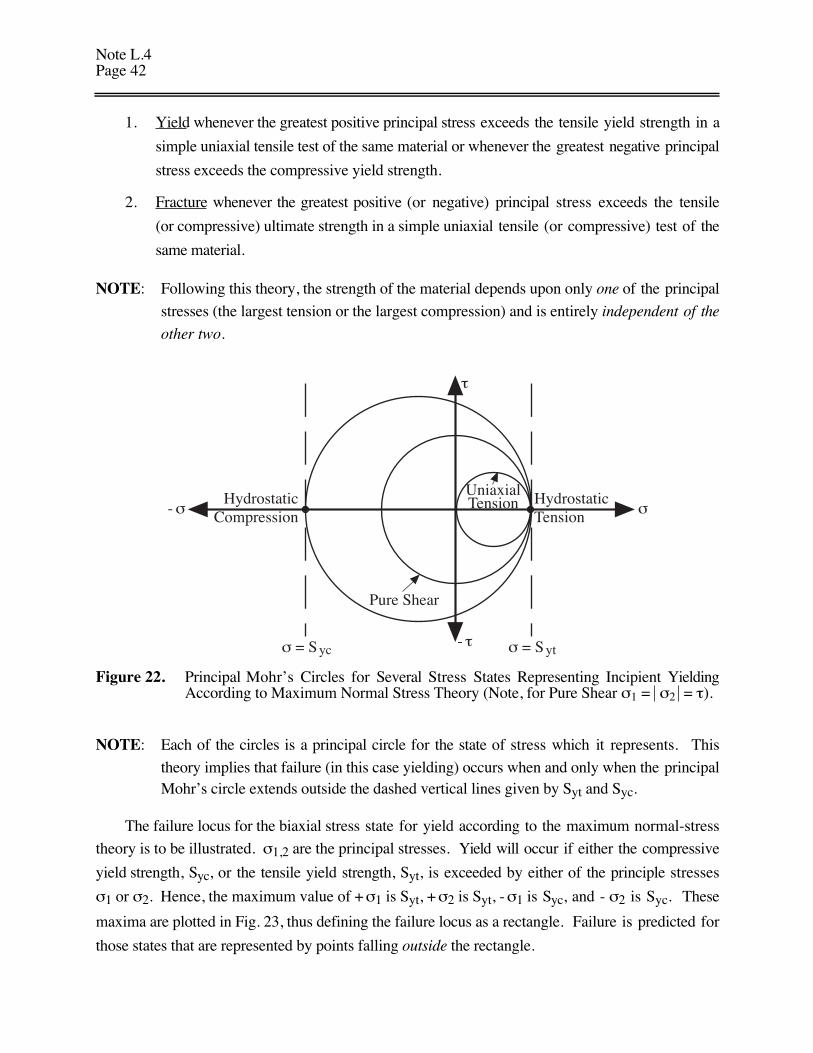
Figure 22. Principal Mohr’s Circles for Several Stress States Representing Incipient YieldingAccording to Maximum Normal Stress Theory (Note, for Pure Shear σ1 = σ2 = τ).

NOTE: Each of the circles is a principal circle for the state of stress which it represents. This

theory implies that failure (in this case yielding) occurs when and only when the principalMohr’s circle extends outside the dashed vertical lines given by Syt and Syc.

The failure locus for the biaxial stress state for yield according to the maximum normal-stress

theory is to be illustrated. σ1,2 are the principal stresses. Yield will occur if either the compressive

yield strength, Syc, or the tensile yield strength, Syt, is exceeded by either of the principle stresses

σ1 or σ2. Hence, the maximum value of + σ1 is Syt, + σ2 is Syt, - σ1 is Syc, and - σ2 is Syc. These

maxima are plotted in Fig. 23, thus defining the failure locus as a rectangle. Failure is predicted for

those states that are represented by points falling outside the rectangle.

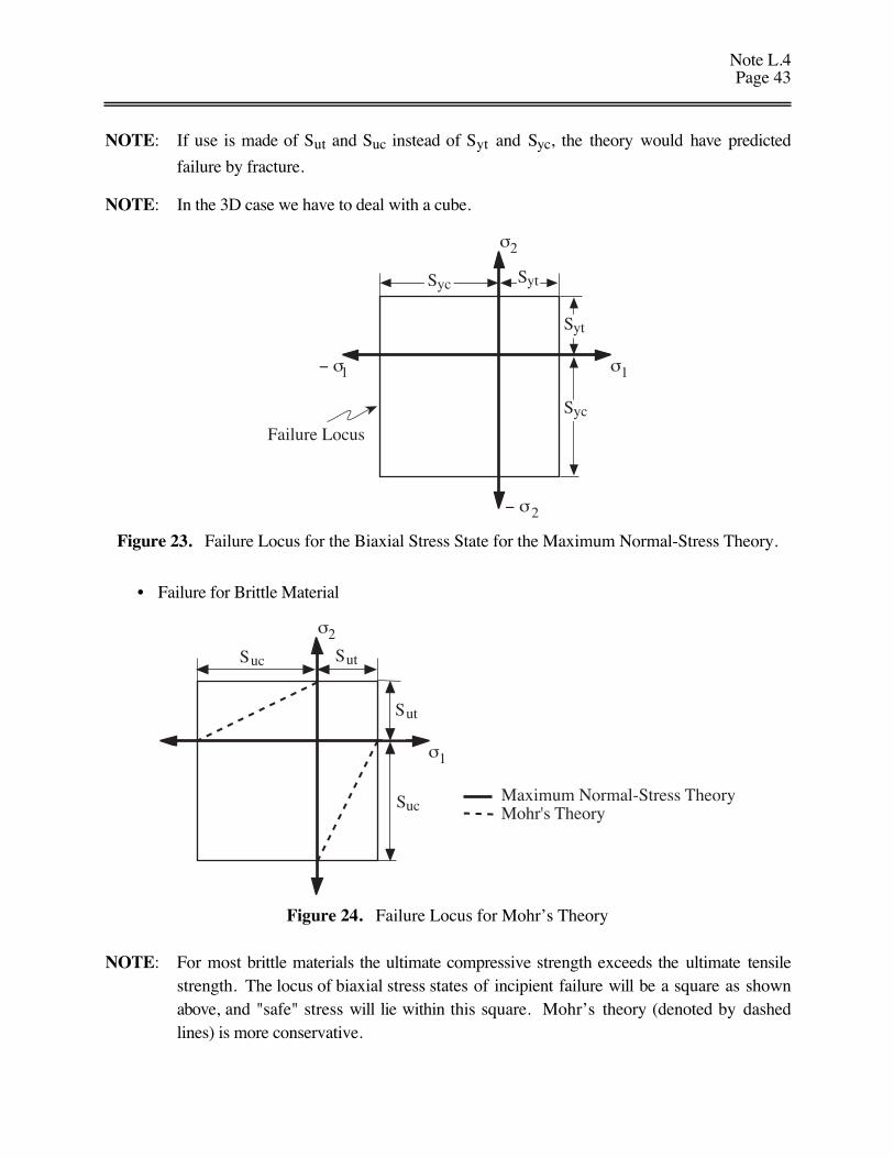
Note L.4Page 43

NOTE: If use is made of Sut and Suc instead of Syt and Syc, the theory would have predicted

failure by fracture.

NOTE: In the 3D case we have to deal with a cube.

Syt

σ2

Syt

Syc

Syc

σ1

− σ2

− σ1

Failure Locus

Figure 23. Failure Locus for the Biaxial Stress State for the Maximum Normal-Stress Theory.

• Failure for Brittle Material

σ2

Mohr's TheoryMaximum Normal-Stress Theory

σ1

Suc Sut

Sut

Suc

Figure 24. Failure Locus for Mohr’s Theory

NOTE: For most brittle materials the ultimate compressive strength exceeds the ultimate tensilestrength. The locus of biaxial stress states of incipient failure will be a square as shownabove, and "safe" stress will lie within this square. Mohr’s theory (denoted by dashedlines) is more conservative.

Note L.4Page 44

It is often convenient to refer to an equivalent stress, Se (σe), as calculated by some

particular theory.

NOTE: The equivalent stress may or may not be equal to the yield strength.

Mathematically, the equivalent stress based on the maximum stress theory is given by:

Se = σi max i = 1, 2, 3 (6.1)

Applicability of Method –

Reasonably accurate for materials which produce brittle fracture both in the test specimen

and in actual service such as: Cast iron, concrete, hardened tool steel, glass [Ref. 3, Fig. 6.8].

It cannot predict failure under hydrostatic compression (the state of stress in which all three

principle stresses are equal). Structural materials, including those listed above, can withstand

hydrostatic stresses many times Suc.

It cannot accurately predict strengths where a ductile failure occurs.

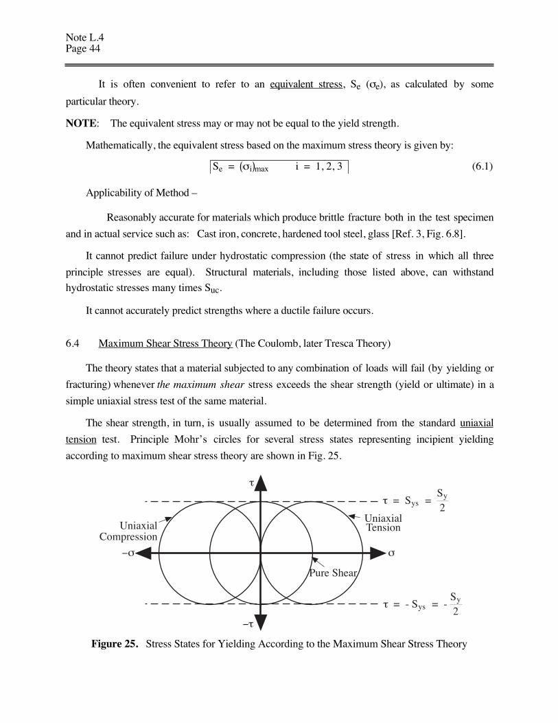
6.4 Maximum Shear Stress Theory (The Coulomb, later Tresca Theory)

The theory states that a material subjected to any combination of loads will fail (by yielding or

fracturing) whenever the maximum shear stress exceeds the shear strength (yield or ultimate) in a

simple uniaxial stress test of the same material.

The shear strength, in turn, is usually assumed to be determined from the standard uniaxial

tension test. Principle Mohr’s circles for several stress states representing incipient yielding

according to maximum shear stress theory are shown in Fig. 25.

Uniaxial Compression

Uniaxial Tension

τ

σ

Pure Shear

−σ

−τ

τ = Sys = Sy

2

τ = - Sys = - Sy

2

Figure 25. Stress States for Yielding According to the Maximum Shear Stress Theory

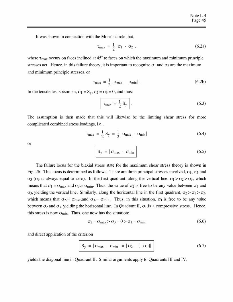
Note L.4Page 45

It was shown in connection with the Mohr’s circle that,

τmax = 12

σ1 - σ2 , (6.2a)

where τmax occurs on faces inclined at 45˚ to faces on which the maximum and minimum principle

stresses act. Hence, in this failure theory, it is important to recognize σ1 and σ2 are the maximum

and minimum principle stresses, or

τmax = 12

σmax - σmin . (6.2b)

In the tensile test specimen, σ1 = Sy, σ2 = σ3 = 0, and thus:

τmax = 12

Sy . (6.3)

The assumption is then made that this will likewise be the limiting shear stress for more

complicated combined stress loadings, i.e.,

τmax = 12

Sy = 12

σmax - σmin (6.4)

or

Sy = σmax - σmin (6.5)

The failure locus for the biaxial stress state for the maximum shear stress theory is shown in

Fig. 26. This locus is determined as follows. There are three principal stresses involved, σ1, σ2 and

σ3 (σ3 is always equal to zero). In the first quadrant, along the vertical line, σ1 > σ2 > σ3, which

means that σ1 = σmax and σ3.= σmin. Thus, the value of σ2 is free to be any value between σ1 and

σ3, yielding the vertical line. Similarly, along the horizontal line in the first quadrant, σ2 > σ1 > σ3,

which means that σ2.= σmax.and σ3.= σmin. Thus, in this situation, σ1 is free to be any value

between σ2 and σ3, yielding the horizontal line. In Quadrant II, σ1.is a compressive stress. Hence,

this stress is now σmin. Thus, one now has the situation:

σ2 = σmax > σ3 = 0 > σ1 = σmin (6.6)

and direct application of the criterion

Sy = σmax - σmin = σ2 - - σ1 (6.7)

yields the diagonal line in Quadrant II. Similar arguments apply to Quadrants III and IV.

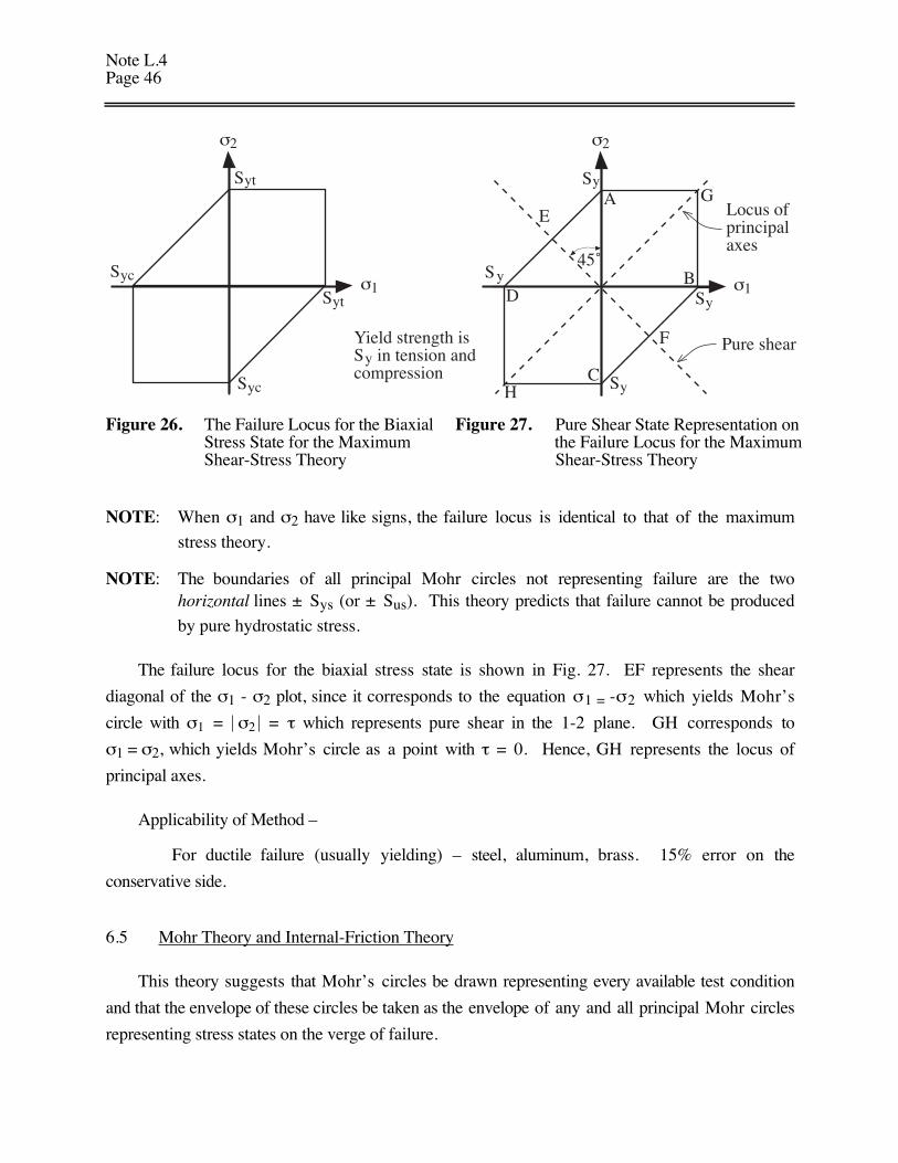
Note L.4Page 46

ytS

ytSycS

ycS

2σ

1σ

Yield strength is S in tension and compression

y

yS

ySyS

yS

2σ

1σ

A

B

C

D

E

F

G

H

45˚

Locus of principal axes

Pure shear

Figure 26. The Failure Locus for the Biaxial Figure 27. Pure Shear State Representation onStress State for the Maximum the Failure Locus for the MaximumShear-Stress Theory Shear-Stress Theory

NOTE: When σ1 and σ2 have like signs, the failure locus is identical to that of the maximum

stress theory.

NOTE: The boundaries of all principal Mohr circles not representing failure are the twohorizontal lines ± Sys (or ± Sus). This theory predicts that failure cannot be produced

by pure hydrostatic stress.

The failure locus for the biaxial stress state is shown in Fig. 27. EF represents the shear

diagonal of the σ1 - σ2 plot, since it corresponds to the equation σ1 = -σ2 which yields Mohr’s

circle with σ1 = σ2 = τ which represents pure shear in the 1-2 plane. GH corresponds to

σ1 = σ2, which yields Mohr’s circle as a point with τ = 0. Hence, GH represents the locus of

principal axes.

Applicability of Method –

For ductile failure (usually yielding) – steel, aluminum, brass. 15% error on the

conservative side.

6.5 Mohr Theory and Internal-Friction Theory

This theory suggests that Mohr’s circles be drawn representing every available test condition

and that the envelope of these circles be taken as the envelope of any and all principal Mohr circles

representing stress states on the verge of failure.

Note L.4Page 47

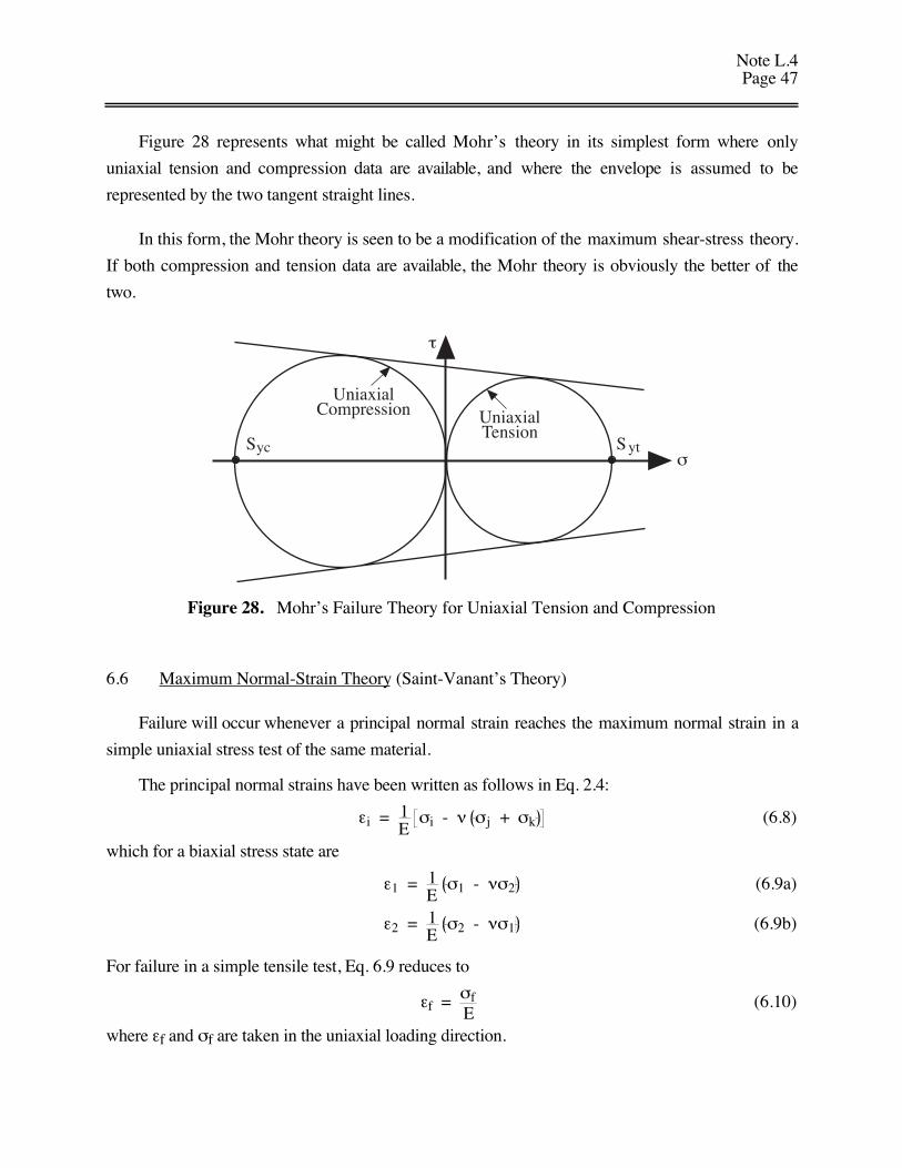
Figure 28 represents what might be called Mohr’s theory in its simplest form where only

uniaxial tension and compression data are available, and where the envelope is assumed to be

represented by the two tangent straight lines.

In this form, the Mohr theory is seen to be a modification of the maximum shear-stress theory.

If both compression and tension data are available, the Mohr theory is obviously the better of the

two.

τ

σS ytSyc

Uniaxial Compression Uniaxial

Tension

Figure 28. Mohr’s Failure Theory for Uniaxial Tension and Compression

6.6 Maximum Normal-Strain Theory (Saint-Vanant’s Theory)

Failure will occur whenever a principal normal strain reaches the maximum normal strain in a

simple uniaxial stress test of the same material.

The principal normal strains have been written as follows in Eq. 2.4:

εi = 1E

σi - ν σj + σk (6.8)

which for a biaxial stress state are

ε1 = 1E

σ1 - νσ2 (6.9a)

ε2 = 1E

σ2 - νσ1 (6.9b)

For failure in a simple tensile test, Eq. 6.9 reduces to

εf = σfE

(6.10)

where εf and σf are taken in the uniaxial loading direction.

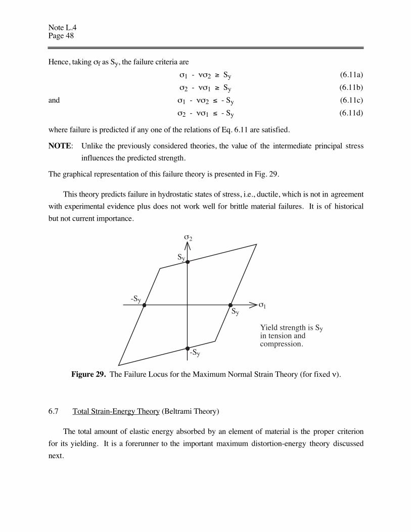
Note L.4Page 48

Hence, taking σf as Sy, the failure criteria are

σ1 - νσ2 ≥ Sy (6.11a)

σ2 - νσ1 ≥ Sy (6.11b)

and σ1 - νσ2 ≤ - Sy (6.11c)

σ2 - νσ1 ≤ - Sy (6.11d)

where failure is predicted if any one of the relations of Eq. 6.11 are satisfied.

NOTE: Unlike the previously considered theories, the value of the intermediate principal stress

influences the predicted strength.

The graphical representation of this failure theory is presented in Fig. 29.

This theory predicts failure in hydrostatic states of stress, i.e., ductile, which is not in agreement

with experimental evidence plus does not work well for brittle material failures. It is of historical

but not current importance.

Sy

σ

-Sy

2

σ1Sy

-Sy

Yield strength is S in tension and compression.

y

Figure 29. The Failure Locus for the Maximum Normal Strain Theory (for fixed ν).

6.7 Total Strain-Energy Theory (Beltrami Theory)

The total amount of elastic energy absorbed by an element of material is the proper criterion

for its yielding. It is a forerunner to the important maximum distortion-energy theory discussed

next.

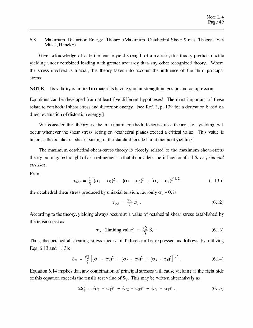
Note L.4Page 49

6.8 Maximum Distortion-Energy Theory (Maximum Octahedral-Shear-Stress Theory, VanMises, Hencky)

Given a knowledge of only the tensile yield strength of a material, this theory predicts ductile

yielding under combined loading with greater accuracy than any other recognized theory. Where

the stress involved is triaxial, this theory takes into account the influence of the third principal

stress.

NOTE: Its validity is limited to materials having similar strength in tension and compression.

Equations can be developed from at least five different hypotheses! The most important of these

relate to octahedral shear stress and distortion energy. [see Ref. 3, p. 139 for a derivation based on

direct evaluation of distortion energy.]

We consider this theory as the maximum octahedral-shear-stress theory, i.e., yielding will

occur whenever the shear stress acting on octahedral planes exceed a critical value. This value is

taken as the octahedral shear existing in the standard tensile bar at incipient yielding.

The maximum octahedral-shear-stress theory is closely related to the maximum shear-stress

theory but may be thought of as a refinement in that it considers the influence of all three principal

stresses.

From

τoct = 13

σ1 - σ22 + σ2 - σ3

2 + σ3 - σ12 1/2 (1.13b)

the octahedral shear stress produced by uniaxial tension, i.e., only σ1 ≠ 0, is

τoct = 23

σ1 . (6.12)

According to the theory, yielding always occurs at a value of octahedral shear stress established by

the tension test as

τoct (limiting value) = 23

Sy . (6.13)

Thus, the octahedral shearing stress theory of failure can be expressed as follows by utilizing

Eqs. 6.13 and 1.13b:

Sy = 22

σ1 - σ22 + σ2 - σ3

2 + σ3 - σ12 1/2 . (6.14)

Equation 6.14 implies that any combination of principal stresses will cause yielding if the right side

of this equation exceeds the tensile test value of Sy. This may be written alternatively as

2Sy2 = σ1 - σ2

2 + σ2 - σ32 + σ3 - σ1

2 . (6.15)

Note L.4Page 50

A variation of Eq. 6.14 which is sometimes useful involves the concept of an equivalent

uniaxial tensile stress, σe, where σe is the value of uniaxial tensile stress which produces the same

level of octahedral shear stress as does the actual combination of existing principal stresses, thus

σe = 22

σ1 - σ22 + σ2 - σ3

2 + σ3 - σ12 1/2 (6.16)

Obviously, if the loads are such that σe > Sy, yielding would be predicted. For design purposes, σe

should be made equal to the allowable working uniaxial stress.

• Case of Pure Biaxial Shear-Stress

Recalling Mohr’s circle for this case, we have the principal stresses

σ1 = τ, σ2 = -τ, σ3 = 0.

Substituting these values into Eqs. 6.14 or 6.16 gives

Sy or σe = 3 τ , (6.17)

This means that if τ > Sy

3 = 0.577 Sy, the material will yield. Hence, according to the maximum

octahedral-shear-stress theory, a material is 57.7% as strong in shear as it is in tension.

• General Case of Biaxial Stress (σ3 = 0)

Equation 6.16 reduces to

σe = σ12 + σ2

2 - σ1σ21/2

(6.18)

In many biaxial-stress problems it is more convenient to work directly with stress σx, σy and

τxy, because these can be determined more readily than principal stresses. Equation 6.18 can be

modified for this purpose by application of Eq. 1.8 to yield Eq. 6.19:

σ1, σ2 = σx + σy

2 ± τxy

2 + σx - σy

2

2(1.8)

σe = σx2 + σy

2 - σxσy + 3τxy2 1/2 (6.19)

Equation 6.19 can also be derived by superposition of Eqs. 6.17 and 6.18.

The locus of failure conditions for this failure theory is illustrated by the ellipse in Fig. 30.

NOTE: The theory can be independently developed from the maximum distortion-energy theory,

which postulates that failure (yielding) is caused by the elastic energy associated with this

distortion.

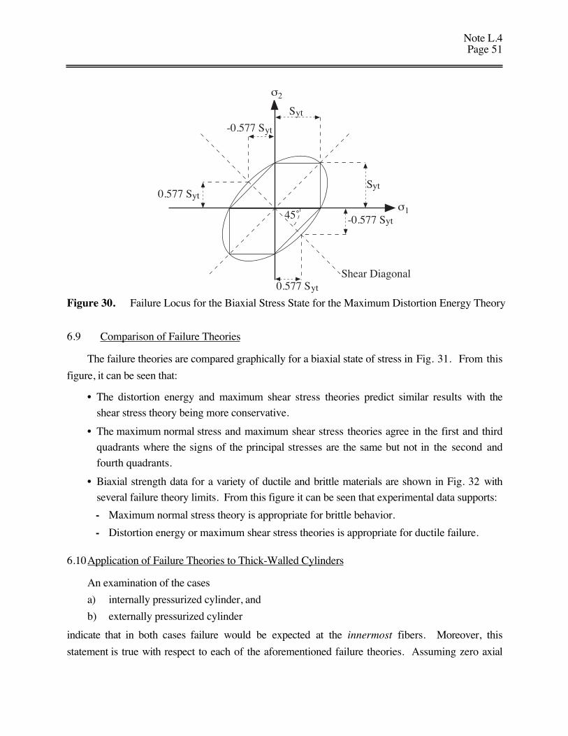
Note L.4Page 51

45˚

σ2

σ1

Shear Diagonal

-0.577 S

S

-0.577 S

0.577 SS

0.577 S

yt

yt

yt

yt

yt

yt

Figure 30. Failure Locus for the Biaxial Stress State for the Maximum Distortion Energy Theory

6.9 Comparison of Failure Theories

The failure theories are compared graphically for a biaxial state of stress in Fig. 31. From this

figure, it can be seen that:

• The distortion energy and maximum shear stress theories predict similar results with the

shear stress theory being more conservative.

• The maximum normal stress and maximum shear stress theories agree in the first and third

quadrants where the signs of the principal stresses are the same but not in the second and

fourth quadrants.

• Biaxial strength data for a variety of ductile and brittle materials are shown in Fig. 32 with

several failure theory limits. From this figure it can be seen that experimental data supports:

- Maximum normal stress theory is appropriate for brittle behavior.

- Distortion energy or maximum shear stress theories is appropriate for ductile failure.

6.10Application of Failure Theories to Thick-Walled Cylinders

An examination of the cases

a) internally pressurized cylinder, and

b) externally pressurized cylinder

indicate that in both cases failure would be expected at the innermost fibers. Moreover, this

statement is true with respect to each of the aforementioned failure theories. Assuming zero axial

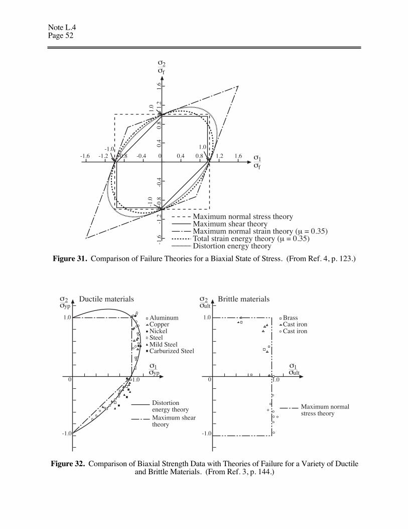
Note L.4Page 52

σ2σf

-1.6 -1.2 -0.8 -0.4-1.0

0 0.4 0.8 1.2 1.6

1.00.4

0.8

1.2

1.6

1.0

-1.6

-1.2

-0.8

-0.4

-1.0

σ1σf

Maximum normal stress theoryMaximum shear theoryMaximum normal strain theory (µ = 0.35)Total strain energy theory (µ = 0.35)Distortion energy theory

Figure 31. Comparison of Failure Theories for a Biaxial State of Stress. (From Ref. 4, p. 123.)

1.0

-1.0

0 1.0

2ult

σσ

1ult

σσ

BrassCast ironCast iron

Maximum normalstress theory

Brittle materials

1.0

-1.0

0 1.0

2yp

σσ

1yp

σσ

Ductile materials

AluminumCopperNickelSteelMild SteelCarburized Steel

Distortionenergy theoryMaximum sheartheory

Figure 32. Comparison of Biaxial Strength Data with Theories of Failure for a Variety of Ductileand Brittle Materials. (From Ref. 3, p. 144.)

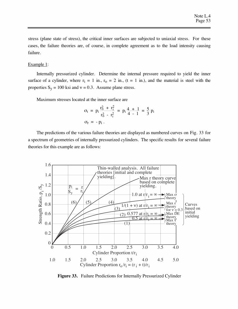
Note L.4Page 53

stress (plane state of stress), the critical inner surfaces are subjected to uniaxial stress. For these

cases, the failure theories are, of course, in complete agreement as to the load intensity causing

failure.

Example 1:

Internally pressurized cylinder. Determine the internal pressure required to yield the inner

surface of a cylinder, where ri = 1 in., ro = 2 in., (t = 1 in.), and the material is steel with the

properties Sy = 100 ksi and ν = 0.3. Assume plane stress.

Maximum stresses located at the inner surface are

σt = pi ro2 + ri

2

ro2 - ri2

= pi 4 + 14 - 1

= 53

pi

σr = - pi .

The predictions of the various failure theories are displayed as numbered curves on Fig. 33 for

a spectrum of geometries of internally pressurized cylinders. The specific results for several failure

theories for this example are as follows:

1.6

1.4

1.2

1.0

0.8

0.6

0.4

0.2

00 0.5 1.0 1.5 2.0 2.5 3.0 3.5 4.0

Stre

ngth

Rat

io, p

/S

iy

1.0 1.5 2.0 2.5 3.0 3.5 4.0 4.5 5.0

Cylinder Proportion t/ri

Cylinder Proportion r /r = (r + t)/ri iio

Thin-walled analysis. All failure theories [initial and complete yielding]. Max r theory curve

based on complete yielding.pi

Sy = r

ri

(6) (5) (4)(3)

(2)

(1)

1.0 at r/r = ∞i Max σ theory

1/(1 + ν) at r/r = ∞i

i0.577 at r/r = ∞ Max DE theoryMax τ theory

Max ε theory for ν = 0.3

Curves based on initial yielding0.5 at r/r = ∞i

Figure 33. Failure Predictions for Internally Pressurized Cylinder

Note L.4Page 54

Curve (1)

According to the maximum shear-stress theory, yielding will begin when the highest shearstress in the cylinder reaches that in the standard tensile test at initial yielding, which is Sy/2. Thus,

τmax = Sy

2or

σt - σr2

= 50 ksi ,

43

pi = 50 ksi

or pi = 37.5 ksi .

Hence, for this case where t/ri = 1.0, pi/Sy = 0.375. This value appears on Fig. 33.

Curve (2)

According to the maximum distortion-energy theory, yielding will begin when the equivalenttensile stress at the inner cylinder wall reaches the tensile stress in the standard tensile test at initialyielding, which is Sy. Hence, using Eq. 6.18 and the known principal stresses:

σe = Sy

σt2 + σr

2 - σtσr1/2

= 100 ksi

53

pi2 + - pi

2 - - 53

pi2 1/2

= 100 ksi

2.33 pi = 100 ksi

or pi = 43 ksi for t/ri = 1.0

Curve (4)

According to the maximum normal-stress theory, yielding will begin when the highest normalstress in the cylinder reaches the highest normal stress in the standard tensile test at initial yielding,which is Sy. Hence,

σt = Sy

5/3 pi = 100 ksi

or the internal pressure required to yield the inner surface is

pi = 60 ksi for t/ri = 1.0.

For the full range of cylindrical geometries, pi can be determined for each theory and is presented

on Fig. 33.

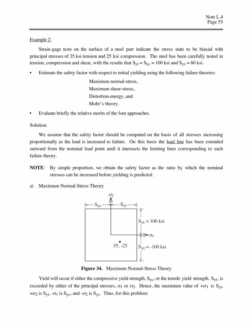
Note L.4Page 55

Example 2:

Strain-gage tests on the surface of a steel part indicate the stress state to be biaxial with

principal stresses of 35 ksi tension and 25 ksi compression. The steel has been carefully tested intension, compression and shear, with the results that Syt = Syc = 100 ksi and Sys = 60 ksi.

• Estimate the safety factor with respect to initial yielding using the following failure theories:

Maximum normal-stress,

Maximum shear-stress,

Distortion-energy, and

Mohr’s theory.

• Evaluate briefly the relative merits of the four approaches.

Solution:

We assume that the safety factor should be computed on the basis of all stresses increasing

proportionally as the load is increased to failure. On this basis the load line has been extended

outward from the nominal load point until it intersects the limiting lines corresponding to each

failure theory.

NOTE: By simple proportion, we obtain the safety factor as the ratio by which the nominal

stresses can be increased before yielding is predicted.

a) Maximum Normal-Stress Theory

Syt

35, -25

σ2

σ1

Syt = 100 ksi

Syc = -100 ksi

Syc

Figure 34. Maximum Normal-Stress Theory

Yield will occur if either the compressive yield strength, Syc, or the tensile yield strength, Syt, is

exceeded by either of the principal stresses, σ1 or σ2. Hence, the maximum value of +σ1 is Syt,

+σ2 is Syt, -σ1 is Syc, and -σ2 is Syc. Thus, for this problem:

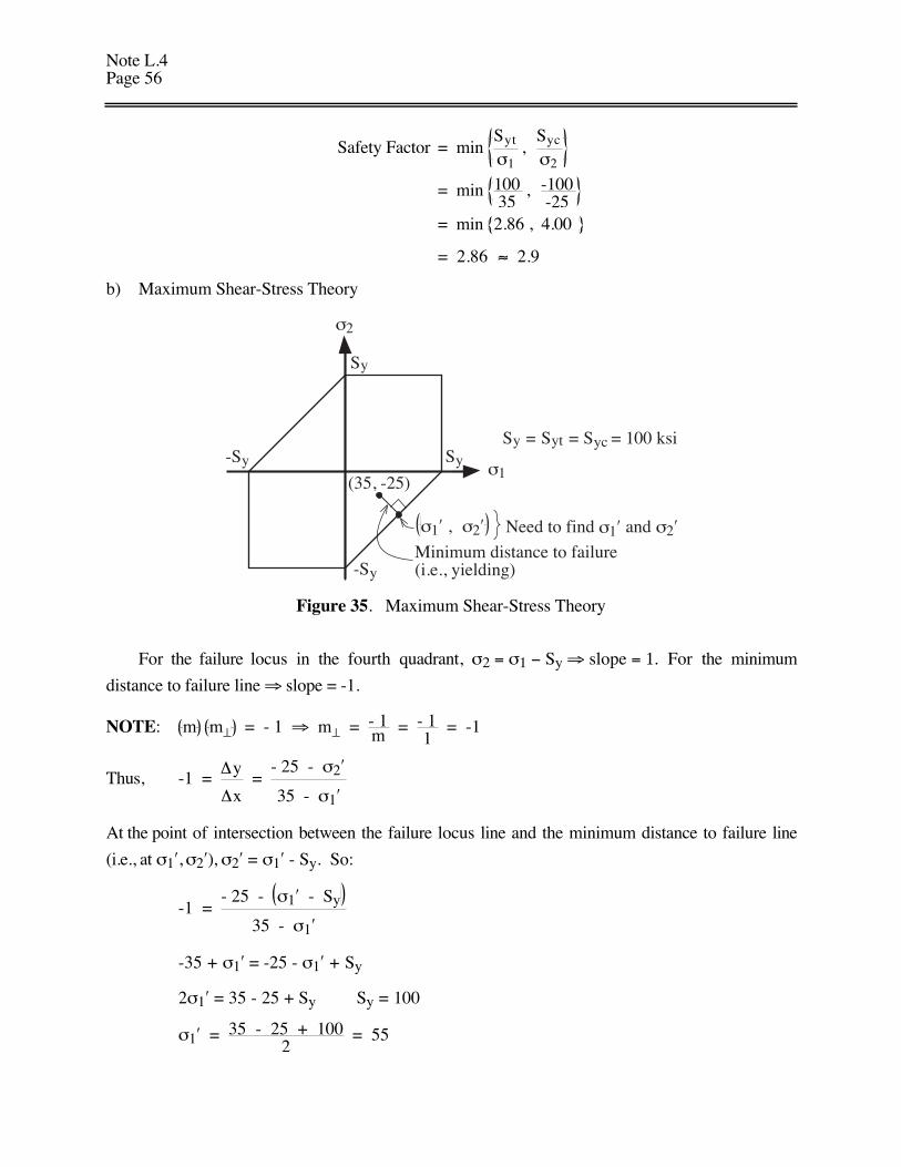
Note L.4Page 56

Safety Factor = min Syt

σ1 ,

Syc

σ2

= min 10035

, -100-25

= min 2.86 , 4.00

= 2.86 ≈ 2.9

b) Maximum Shear-Stress Theory

yS

ySy-S

y-S

2σ

1σ(35, -25)

Minimum distance to failure (i.e., yielding)

σ1′ , σ2′

ytS = ycS = 100 ksiyS =

Need to find andσ1′ σ2′

Figure 35. Maximum Shear-Stress Theory

For the failure locus in the fourth quadrant, σ2 = σ1 − Sy ⇒ slope = 1. For the minimum

distance to failure line ⇒ slope = -1.

NOTE: m m⊥ = - 1 ⇒ m⊥ = - 1m = - 11

= -1

Thus, -1 = ∆y

∆x =

- 25 - σ2′

35 - σ1′

At the point of intersection between the failure locus line and the minimum distance to failure line

(i.e., at σ1′, σ2′), σ2′ = σ1′ - Sy. So:

-1 = - 25 - σ1′ - Sy

35 - σ1′

-35 + σ1′ = -25 - σ1′ + Sy

2σ1′ = 35 - 25 + Sy Sy = 100

σ1′ = 35 - 25 + 1002

= 55

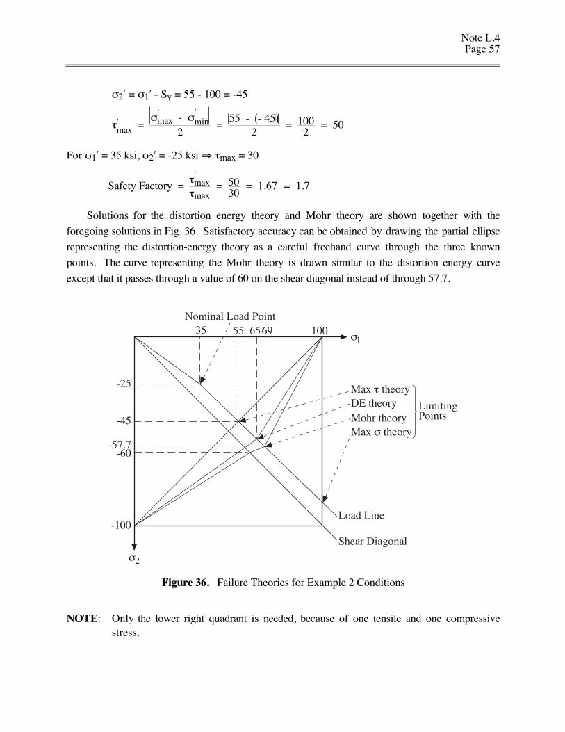
Note L.4Page 57

σ2′ = σ1′ - Sy = 55 - 100 = -45

τmax′ =

σmax′ - σmin

′

2 =

55 - - 452

= 1002

= 50

For σ1′ = 35 ksi, σ2′ = -25 ksi ⇒ τmax = 30

Safety Factory = τmax

′

τmax = 50

30 = 1.67 ≈ 1.7

Solutions for the distortion energy theory and Mohr theory are shown together with the

foregoing solutions in Fig. 36. Satisfactory accuracy can be obtained by drawing the partial ellipse

representing the distortion-energy theory as a careful freehand curve through the three known

points. The curve representing the Mohr theory is drawn similar to the distortion energy curve

except that it passes through a value of 60 on the shear diagonal instead of through 57.7.

σ2

σ1

Load Line

Shear Diagonal

35

-25

-57.7-60

-100

55 6569 100Nominal Load Point

Max τ theoryDE theoryMohr theoryMax σ theory

Limiting Points-45

Figure 36. Failure Theories for Example 2 Conditions

NOTE: Only the lower right quadrant is needed, because of one tensile and one compressivestress.

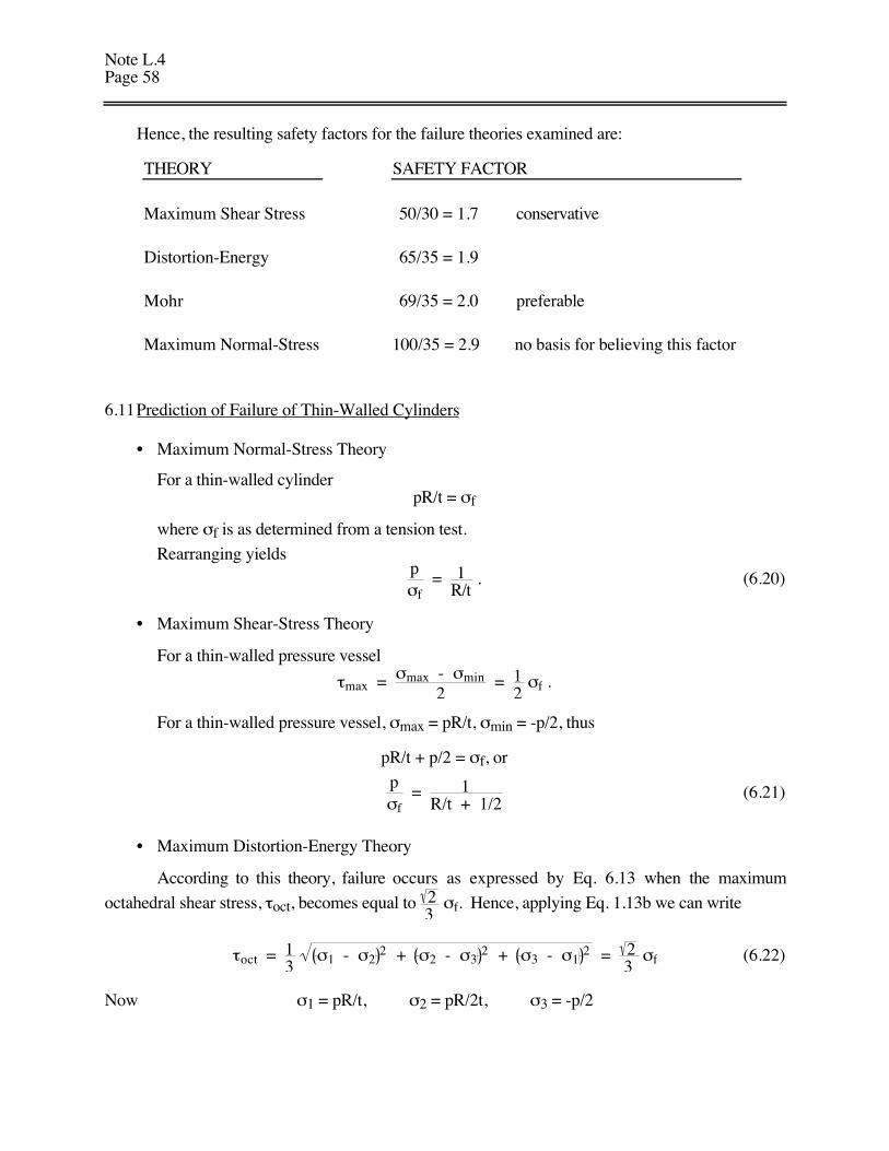
Note L.4Page 58

Hence, the resulting safety factors for the failure theories examined are:

THEORY SAFETY FACTOR

Maximum Shear Stress 50/30 = 1.7 conservative

Distortion-Energy 65/35 = 1.9

Mohr 69/35 = 2.0 preferable

Maximum Normal-Stress 100/35 = 2.9 no basis for believing this factor

6.11Prediction of Failure of Thin-Walled Cylinders

• Maximum Normal-Stress Theory

For a thin-walled cylinderpR/t = σf

where σf is as determined from a tension test.

Rearranging yieldspσf

= 1R/t

. (6.20)

• Maximum Shear-Stress Theory

For a thin-walled pressure vessel

τmax = σmax - σmin2

= 12

σf .

For a thin-walled pressure vessel, σmax = pR/t, σmin = -p/2, thus

pR/t + p/2 = σf, or

pσf

= 1R/t + 1/2

(6.21)

• Maximum Distortion-Energy Theory

According to this theory, failure occurs as expressed by Eq. 6.13 when the maximum

octahedral shear stress, τoct, becomes equal to 23

σf. Hence, applying Eq. 1.13b we can write

τoct = 13

σ1 - σ22 + σ2 - σ3

2 + σ3 - σ12 = 2

3 σf (6.22)

Now σ1 = pR/t, σ2 = pR/2t, σ3 = -p/2

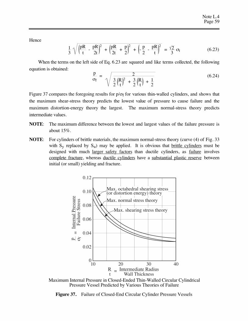
Note L.4Page 59

Hence

13

pRt

- pR2t

2 +

pR2t

+ p2

2 + -

p2

- pR

t

2 = 2

3 σf (6.23)

When the terms on the left side of Eq. 6.23 are squared and like terms collected, the following

equation is obtained:pσf

= 232

Rt

2 + 3

2 R

t + 1

2

(6.24)

Figure 37 compares the foregoing results for p/σf for various thin-walled cylinders, and shows that

the maximum shear-stress theory predicts the lowest value of pressure to cause failure and the

maximum distortion-energy theory the largest. The maximum normal-stress theory predicts

intermediate values.

NOTE: The maximum difference between the lowest and largest values of the failure pressure isabout 15%.

NOTE: For cylinders of brittle materials, the maximum normal-stress theory (curve (4) of Fig. 33with Sy replaced by Su) may be applied. It is obvious that brittle cylinders must bedesigned with much larger safety factors than ductile cylinders, as failure involvescomplete fracture, whereas ductile cylinders have a substantial plastic reserve betweeninitial (or small) yielding and fracture.

100

20

0.02

30

0.04

40

0.06

0.08

0.10

0.12

p σf =

Int

erna

l Pre

ssur

eFa

ilure

Str

ess

Rt

= Intermediate RadiusWall Thickness

Max. normal stress theory

Max. shearing stress theory

Max. octahedral shearing stress (or distortion energy) theory

Maximum Internal Pressure in Closed-Ended Thin-Walled Circular CylindricalPressure Vessel Predicted by Various Theories of Failure

Figure 37. Failure of Closed-End Circular Cylinder Pressure Vessels

Note L.4Page 60

6.12Examples for the Calculation of Safety Factors in Thin-Walled Cylinders

Example:

The most stressed volume element of a certain load-carrying member is located at the free

surface. With the xy plane tangent to the free surface, the stress components were found to be

σx = 15,000 psi

σy = -2,000 psi

τxy = 7,000 psi

The load-stress relations for the member are linear so that the safety factor, N, can be applied eitherto loads or stresses. Determine N if the member is made of a ductile metal with a tensile yieldstress of σe = 44,000 psi.

NOTE: In general N ≡ Yield StressLoad Stress

. Hence, we can write N(Load Stress) ≡ Yield Stress.

1) Maximum Distortion-Energy Theory – From Eq. 6.12 together with the definition of N weobtain:

N τoct = 23

Sy

For a uniaxial tensile test σe = Sy. Also, τoct is given by Eq. 1.14b for stresses in the general x,y, z directions. Hence, the above equation becomes:

N3

σx - σy2 + σy - σz

2 + σz - σx2 + 6 τxy

2 + τxz 2 + τyz

2 2 1/2 = 2

3 (44,000)

For the given stress components obtain:

N3

17,000 2 + - 2,000 2 + - 15,000 2 + 6 7,000 2 = 23

(44,000)

N 812 ⋅ 106

= 2 (44,000)

N = 2.18

NOTE: This result can also be obtained directly from the result for a biaxial stress state,Eq. 6.19 as:

N σx 2 + σy

2 - σxσy + 3τxy 2 1/2 = σe

N 15,000 2 + - 2,000 2 + 30 ⋅ 106 + 3 7,000 2 1/2 = 44,000

N 406 ⋅ 106 = 44,000

N = 2.18

2) Maximum Shear-Stress Theory – In order to use this theory it is necessary to determine thethree principal stresses. From Mohr’s circle:

Note L.4Page 61

σ1 = σx + σy

2 +

σx - σy

2

2 + τxy

2

= 12

(13,000) + 14

(17,000) 2 + (7,000) 2

= 6,500 + 11,010

= 17,510 psi

σ2 = 6,500 - 11,010

= - 4,510 psiσ3 = 0

At failure the three principal stresses are:

σ1 = 17,510 N psi

σ2 = - 4,510 N psi

σ3 = 0

Now, from Eq. 6.5, which expresses the failure criterion for the maximum shear stress theory:

17,520 N + 4,510 N = 44,000

N ≈ 2

If the maximum distortion-energy theory is used, the loads can be increased by a factor of 2.18

before failure by general yielding. Assuming this is correct, the maximum shear-stress theory

of failure is conservative since it predicts smaller failure loads.

REFERENCES

[1] S.H. Crandall, N.C. Dahl and T.J. Lardner, An Introduction to the Mechanics of Solids,

McGraw-Hill, 2nd ed., 1972.

[2] P.L. Pfenningwerth, “Stress Analysis with Applications to Pressurized Water Reactors,”

Report #TID-4500 (16th Ed.), Bettis Atomic Power Laboratory, Pittsburgh, PA, January,

1963. Alternately, see Chapter 4 of J.F. Harvey, Theory and Design of Pressure Vessels,

Van Nostrand Reinhold Co., New York, 1985.

[3] J.A. Collins, Failure of Materials in Mechanical Design – Analysis, Prediction, Prevention,

Wiley, 1981.

[4] J. Marin, Mechanical Behavior of Engineering Materials, Prentice-Hall, Inc., 1962.