Nonparametric Frontier Estimation: recent … Frontier Estimation: recent developments and new...
89
Nonparametric Frontier Estimation: recent developments and new challenges Toulouse - October 2011 Léopold Simar Institut de Statistique Université Catholique de Louvain, Belgium
Transcript of Nonparametric Frontier Estimation: recent … Frontier Estimation: recent developments and new...
'&
$%
Nonparametric Frontier Estimation: recent
developments and new challenges
Toulouse - October 2011
Léopold Simar
Institut de Statistique
Université Catholique de Louvain, Belgium
Nonparametric Frontier Estimation: recent developments and new challenges 2'&
$%
Contents
∙ Frontier Models and Efficiency Measures
– Economy of Production and Farell-Debreu efficiency scores
∙ Statistical Paradigm
– Different models and Different approaches
∙ Nonparametric approaches
– FDH and DEA estimators and Statistical inference
∙ Challenges: Drawbacks of FDH/DEA and Solutions
– Robustness to outliers: Partial-order frontier (order-m and order-� quantile)
– Economic interpretation of the frontier: Parametric approximations
– Hetrogeneity: introducing Environmental Factors
– Introducing noise: Stochastic Nonparametric Frontiers
Nonparametric Frontier Estimation: recent developments and new challenges 3'&
$%
I. Frontier Models and Efficiency Measures
Nonparametric Frontier Estimation: recent developments and new challenges 4'&
$%
The Frontier Model -1-
∙ Economic Theory Koopmans (1951), Debreu (1951): “Activity Analysis”
– x ∈ ℝp+ vector of inputs
– y ∈ ℝq+ vector of outputs
– Production set Ψ of physically attainable points (x, y):
Ψ = {(x, y) ∈ ℝp+q+ ∣ x can produce y}.
∙ The input (output) correspondence sets
– Ψ can be described by its sections:
∀ y ∈ Ψ, X(y) = {x ∈ ℝp+ ∣ (x, y) ∈ Ψ}
∀ x ∈ Ψ, Y (x) = {y ∈ ℝq+ ∣ (x, y) ∈ Ψ}.
– We have
∀(x, y) ∈ Ψ , x ∈ X(y) ⇔ y ∈ Y (x).
Nonparametric Frontier Estimation: recent developments and new challenges 5'&
$%
0 2 4 6 8 10 120
1
2
3
4
5
6
7
8
input: x
outp
ut: y
Production set
y0 X(y
0)
x0
Y(x0)
Ψ
0 2 4 6 8 10 120
2
4
6
8
10
12
input1: x
1
inpu
t 2: x2
Isoquants in input space
X(y1)
X(y2)
y2 > y
1
0 2 4 6 8 10 120
2
4
6
8
10
12
output1: y
1
outp
ut2: y
2
Isoquants in output space
Y(x1)
Y(x2)
x1<x
2
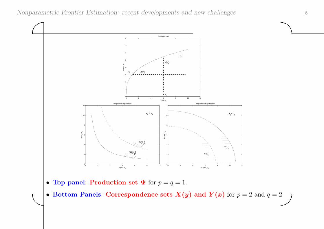
∙ Top panel: Production set Ψ for p = q = 1.
∙ Bottom Panels: Correspondence sets X(y) and Y (x) for p = 2 and q = 2
Nonparametric Frontier Estimation: recent developments and new challenges 6'&
$%
The Frontier Model -2-
∙ Usual Assumptions (a.o.): (Shephard, 1970)
– Free Disposability of inputs and outputs
∀(x, y) ∈ Ψ, then if x′ ≥ x, y′ ≤ y, (x′, y′) ∈ Ψ
– Convexity: if (x1, y1), (x2, y2) ∈ Ψ, then for all � ∈ [0, 1] we have:
(x, y) = �(x1, y1) + (1− �)(x2, y2) ∈ Ψ
– No Free Lunches: (x, y) /∈ Ψ if x = 0 and y ≥ 0, y ∕= 0.
∙ Farrell-Debreu Efficiency scores
radial measures of distance to the boundary of Ψ
– Input oriented: �(x, y) = inf{� ∣ (�x, y) ∈ Ψ} ≤ 1
– Output oriented: �(x, y) = sup{� ∣ (x, �y) ∈ Ψ} ≥ 1
Nonparametric Frontier Estimation: recent developments and new challenges 7'&
$%
0 2 4 6 8 10 120
1
2
3
4
5
6
7
8
input: x
outp
ut: y
Production set
Ψ
P=(x,y) R
Q
M
N
output measure
input measure
0 2 4 6 8 10 120
2
4
6
8
10
12
input1: x
1
inpu
t 2: x2
Isoquants in input space
∂ X(y2)
y2 > y
1
∂ X(y1)
y
P=(x,y1)
Q
O
*
0 2 4 6 8 10 120
2
4
6
8
10
12
output1: y
1ou
tput
2: y2
Isoquants in output space
∂ Y(x2)
∂ Y(x1)
x
P=(x,y2)
Q=(x, y∂ (x) )
•
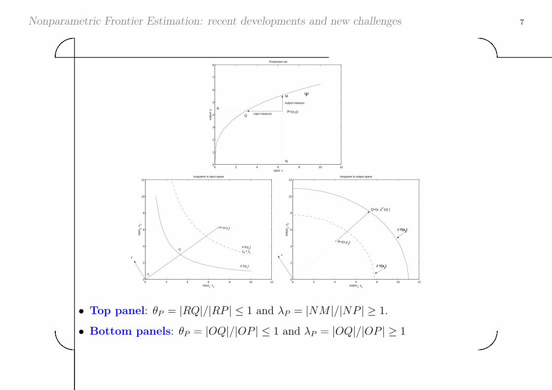
∙ Top panel: �P = ∣RQ∣/∣RP ∣ ≤ 1 and �P = ∣NM ∣/∣NP ∣ ≥ 1.
∙ Bottom panels: �P = ∣OQ∣/∣OP ∣ ≤ 1 and �P = ∣OQ∣/∣OP ∣ ≥ 1
Nonparametric Frontier Estimation: recent developments and new challenges 8'&
$%
The Frontier Model -3-
∙ Extensions
– Hyperbolic Distances: adjusts simultaneously input and output levels
(Färe et al., 1985, Färe and Grosskopf, 2004).
(x, y∣Ψ) = sup{ > 0∣( −1x, y) ∈ Ψ}.
– Directional Distances: Projection of (x, y) onto the technology frontier in a
direction d = (−dx, dy). (Chambers et al., 1998, Färe and Grosskopf, 2000).
�(x, y∣dx, dy,Ψ) = sup{�∣(x − �dx, y + �dy) ∈ Ψ}.
∗ Additive: allow negative values of x and/or y.
∗ Special cases:
⋅ If d = (−x, 0) with x > 0: �(x, y∣dx, dy,Ψ) = 1 − �(x, y∣Ψ)−1
⋅ If d = (0, y) with y > 0: �(x, y∣dx, dy,Ψ) = �(x, y∣Ψ)−1 − 1
Nonparametric Frontier Estimation: recent developments and new challenges 9'&
$%
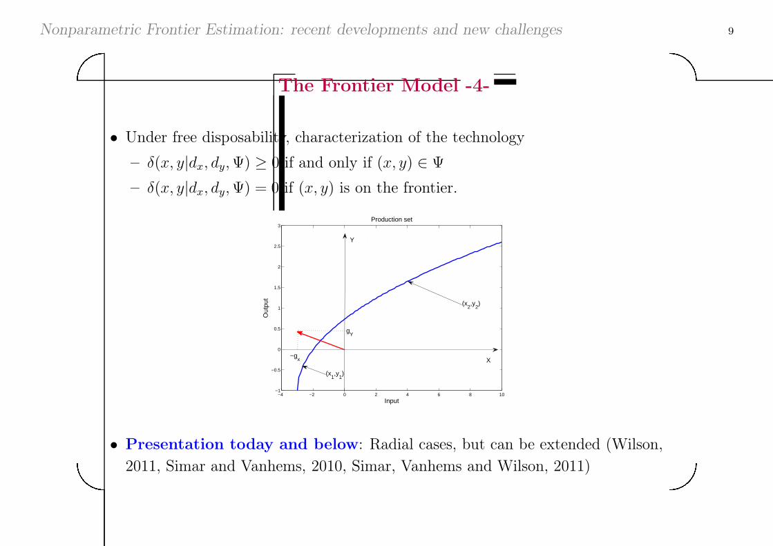
The Frontier Model -4-
∙ Under free disposability, characterization of the technology
– �(x, y∣dx, dy,Ψ) ≥ 0 if and only if (x, y) ∈ Ψ
– �(x, y∣dx, dy,Ψ) = 0 if (x, y) is on the frontier.
−4 −2 0 2 4 6 8 10−1
−0.5
0
0.5
1
1.5
2
2.5
3Production set
Input
Out
put
−gx
gY
Y
X
(x1,y
1)
(x2,y
2)
∙ Presentation today and below: Radial cases, but can be extended (Wilson,
2011, Simar and Vanhems, 2010, Simar, Vanhems and Wilson, 2011)
Nonparametric Frontier Estimation: recent developments and new challenges 10'&
$%
II. The Statistical Paradigm
Nonparametric Frontier Estimation: recent developments and new challenges 11'&
$%
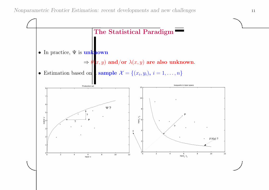
The Statistical Paradigm
∙ In practice, Ψ is unknown
⇒ �(x, y) and/or �(x, y) are also unknown.
∙ Estimation based on a sample X = {(xi, yi), i = 1, . . . , n}
0 2 4 6 8 10 120
1
2
3
4
5
6
7
8
input: x
outp
ut: y
Production set
Ψ ?
• •
•
•
•
•
• •
•
P
?
?
•
0 2 4 6 8 10 120
2
4
6
8
10
12
input1: x
1
inpu
t 2: x2
Isoquants in input space
•
•
• •
•
•
• •
•
•
∂ X(y) ?
?
P
y
Nonparametric Frontier Estimation: recent developments and new challenges 12'&
$%
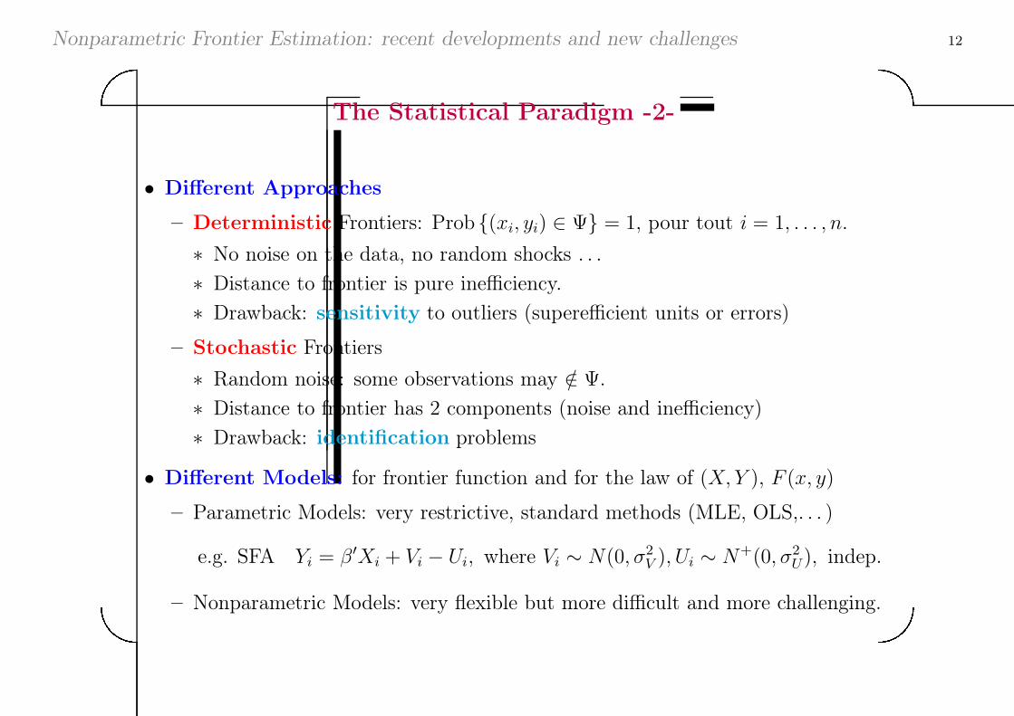
The Statistical Paradigm -2-
∙ Different Approaches
– Deterministic Frontiers: Prob {(xi, yi) ∈ Ψ} = 1, pour tout i = 1, . . . , n.
∗ No noise on the data, no random shocks . . .
∗ Distance to frontier is pure inefficiency.
∗ Drawback: sensitivity to outliers (superefficient units or errors)
– Stochastic Frontiers
∗ Random noise: some observations may /∈ Ψ.
∗ Distance to frontier has 2 components (noise and inefficiency)
∗ Drawback: identification problems
∙ Different Models: for frontier function and for the law of (X, Y ), F (x, y)
– Parametric Models: very restrictive, standard methods (MLE, OLS,. . . )
e.g. SFA Yi = �′Xi + Vi − Ui, where Vi ∼ N(0, �2V ), Ui ∼ N+(0, �2
U), indep.
– Nonparametric Models: very flexible but more difficult and more challenging.
Nonparametric Frontier Estimation: recent developments and new challenges 13'&
$%
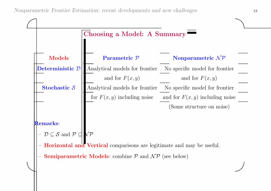
Choosing a Model: A Summary
Models Parametric P Nonparametric NPDeterministic D Analytical models for frontier No specific model for frontier
and for F (x, y) and for F (x, y)
Stochastic S Analytical models for frontier No specific model for frontier
for F (x, y) including noise and for F (x, y) including noise
(Some structure on noise)
Remarks:
– D ⊆ S and P ⊆ NP
– Horizontal and Vertical comparisons are legitimate and may be useful.
– Semiparametric Models: combine P and NP (see below)
Nonparametric Frontier Estimation: recent developments and new challenges 14'&
$%
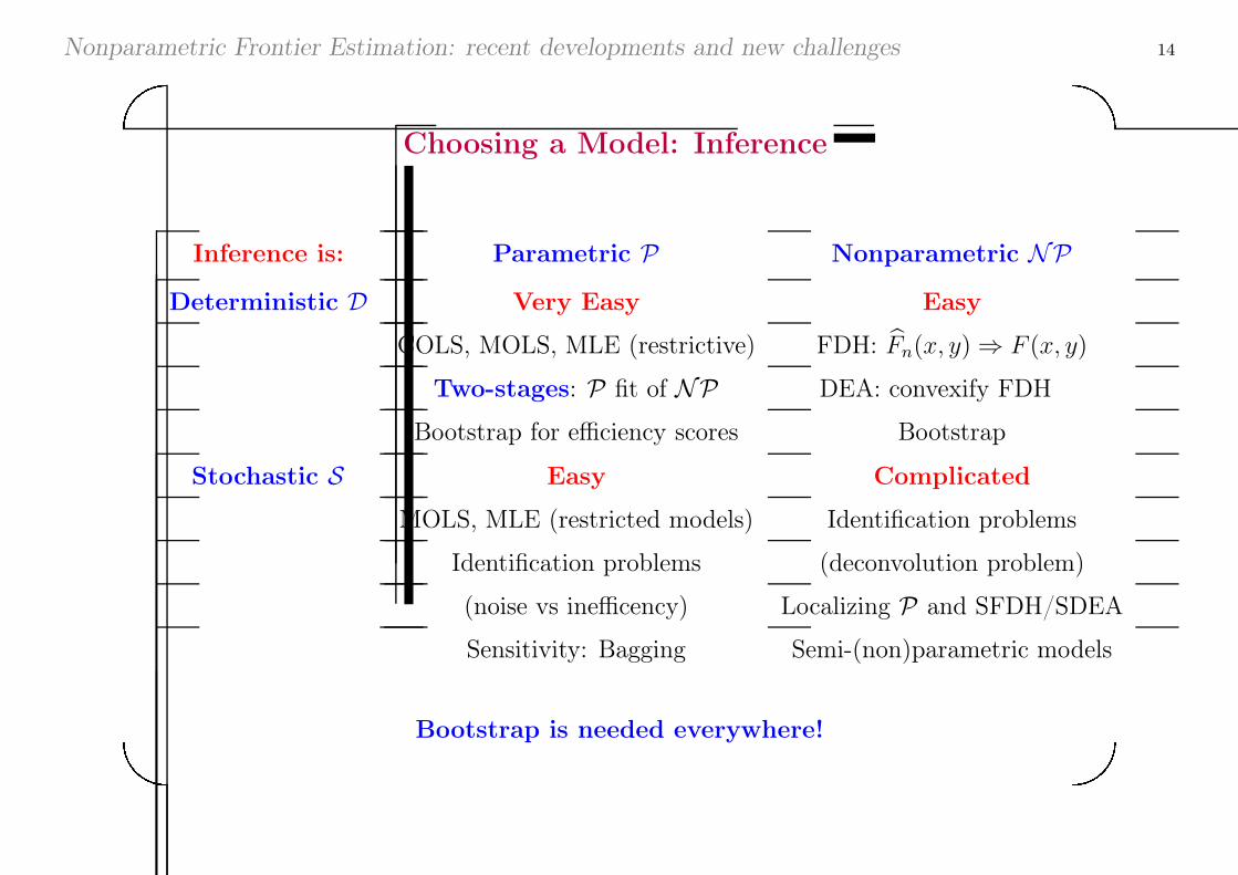
Choosing a Model: Inference
Inference is: Parametric P Nonparametric NPDeterministic D Very Easy Easy
COLS, MOLS, MLE (restrictive) FDH: Fn(x, y) ⇒ F (x, y)
Two-stages: P fit of NP DEA: convexify FDH
Bootstrap for efficiency scores Bootstrap
Stochastic S Easy Complicated
MOLS, MLE (restricted models) Identification problems
Identification problems (deconvolution problem)
(noise vs inefficency) Localizing P and SFDH/SDEA
Sensitivity: Bagging Semi-(non)parametric models
Bootstrap is needed everywhere!
Nonparametric Frontier Estimation: recent developments and new challenges 15'&
$%
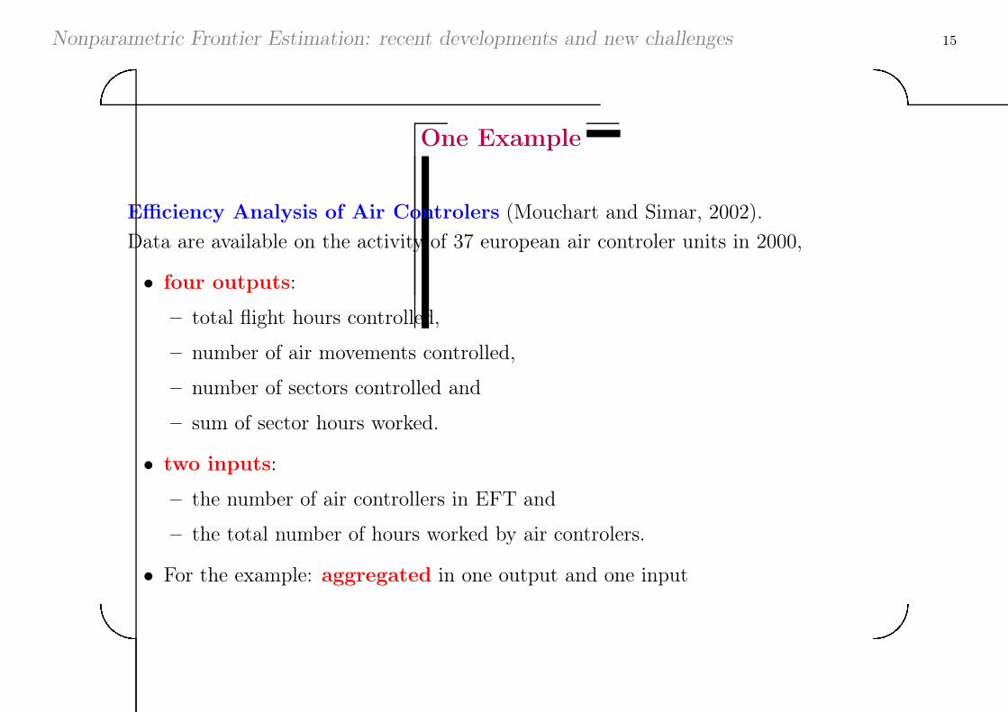
One Example
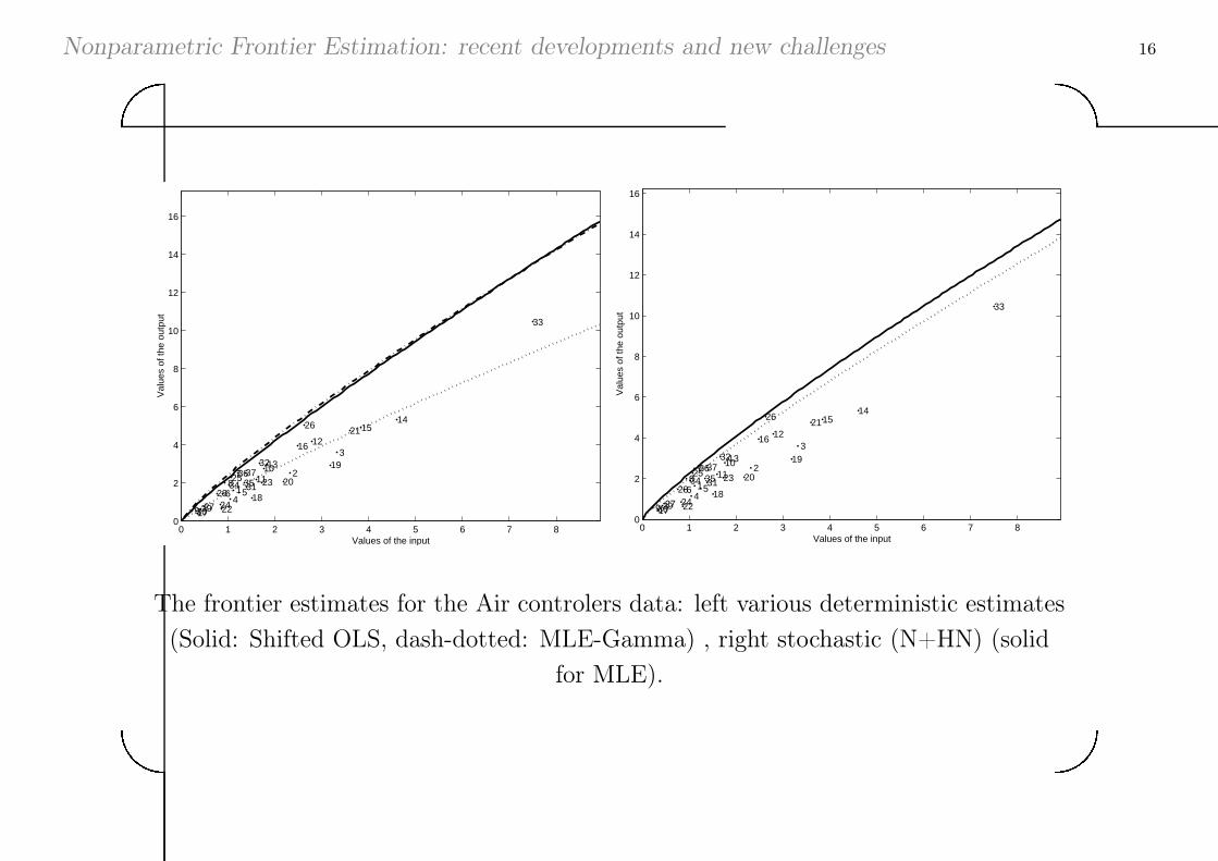
Efficiency Analysis of Air Controlers (Mouchart and Simar, 2002).
Data are available on the activity of 37 european air controler units in 2000,
∙ four outputs:
– total flight hours controlled,
– number of air movements controlled,
– number of sectors controlled and
– sum of sector hours worked.
∙ two inputs:
– the number of air controllers in EFT and
– the total number of hours worked by air controlers.
∙ For the example: aggregated in one output and one input
Nonparametric Frontier Estimation: recent developments and new challenges 16'&
$%
0 1 2 3 4 5 6 7 80
2
4
6
8
10
12
14
16
Values of the input
Val
ues
of th
e ou
tput
1
2
3
4 5 6
7 8
9
1011
12
13
1415
16
17
18
19
20
21
22
23
24
25
26
2728
2930
31
32
33
34 353637
0 1 2 3 4 5 6 7 80
2
4
6
8
10
12
14
16
Values of the input
Val
ues
of th
e ou
tput
1
2
3
4 5 6
7 8
9
1011
12
13
1415
16
17
18
19
20
21
22
23
24
25
26
27
28
2930
31
32
33
34 353637
The frontier estimates for the Air controlers data: left various deterministic estimates
(Solid: Shifted OLS, dash-dotted: MLE-Gamma) , right stochastic (N+HN) (solid
for MLE).
Nonparametric Frontier Estimation: recent developments and new challenges 17'&
$%
0 1 2 3 4 5 6 7 8 9 100
2
4
6
8
10
12
1
2
3
4 5 6
7 8
9
10
11
12
13
1415
16
17
18
19
20
21
22
23
24
25
26
27
28
2930
31
32
33
34 353637
input factor
outp
ut fa
ctor
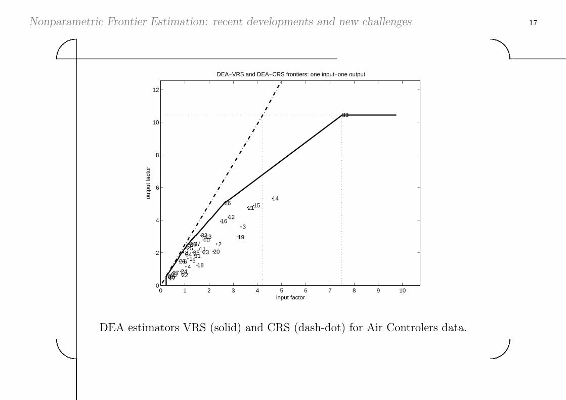
DEA−VRS and DEA−CRS frontiers: one input−one output
DEA estimators VRS (solid) and CRS (dash-dot) for Air Controlers data.
Nonparametric Frontier Estimation: recent developments and new challenges 18'&
$%
The Statistical Paradigm -3-
∙ Statistical Inference
– Estimation individual inefficiencies (“rankings”)
– Confidence intervals for these measures
– Specification tests
∗ Aggregation of inputs and/or outputs
∗ Relevance of the chosen variables
– Hypothesis testing on the shape of the efficient frontier (“technology”)
∗ Convexity
∗ Returns to scale (increasing/decreasing/constant)
– Evolution over time
∗ Panel data
∗ Gain or loss of productivity?
∗ Technical progress or gain of efficiency?
Nonparametric Frontier Estimation: recent developments and new challenges 19'&
$%
The Literature
∙ Parametric deterministic or stochastic frontier models: hundreds of
papers in Econometric literature (Journal of Econometrics,. . . )
Easier but are the parametric assumptions reasonable ones?
∙ Nonparametric deterministic frontier models: thousands of papers in
hundreds of different journals (Management sciences, OR, Econometrics)
Very popular (flexibility) but some drawbacks (see below).
∙ Nonparametric stochastic frontier models: very recent, very few
applications (theoretical econometric literature)
Flexible but so far, hard to use: “work in progress”. . .
∙ Applications: Banks, Transports (Air, Railways,. . . ), Public Services, Municipalities, Post,
School, Education, Research, University, Insurance, Hospitals, Finance, Mutual funds,
Industry, Electric plants, Food industry, Agronomy, Macroeconomic, Economy of development,
Regional economy,. . . (Journal of Productivity Analysis)
Nonparametric Frontier Estimation: recent developments and new challenges 20'&
$%
III. Nonparametric Approaches
Nonparametric Frontier Estimation: recent developments and new challenges 21'&
$%
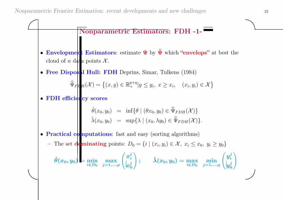
Nonparametric Estimators: FDH -1-
∙ Envelopment Estimators: estimate Ψ by Ψ which “envelops” at best the
cloud of n data points X .
∙ Free Disposal Hull: FDH Deprins, Simar, Tulkens (1984)
ΨFDH(X ) ={(x, y) ∈ ℝ
p+q+ ∣y ≤ yi, x ≥ xi, (xi, yi) ∈ X
}
∙ FDH efficiency scores
�(x0, y0) = inf{� ∣ (�x0, y0) ∈ ΨFDH(X )}�(x0, y0) = sup{� ∣ (x0, �y0) ∈ ΨFDH(X )}.
∙ Practical computations: fast and easy (sorting algorithms)
– The set dominating points: D0 = {i ∣ (xi, yi) ∈ X , xi ≤ x0, yi ≥ y0}
�(x0, y0) = mini∈D0
maxj=1,...,p
(xj
i
xj0
); �(x0, y0) = max
i∈D0
minj=1,...,q
(yj
i
yj0
)
Nonparametric Frontier Estimation: recent developments and new challenges 22'&
$%
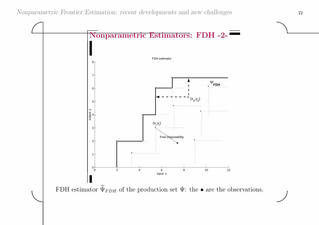
Nonparametric Estimators: FDH -2-
0 2 4 6 8 10 120
1
2
3
4
5
6
7
8
input: x
outp
ut: y
FDH estimator
•
•
•
•
•
•
•
•
•
Free Disposability
•
(xi,y
i)
° (x0,y
0)
ΨFDH
FDH estimator ΨFDH of the production set Ψ: the ∙ are the observations.
Nonparametric Frontier Estimation: recent developments and new challenges 23'&
$%
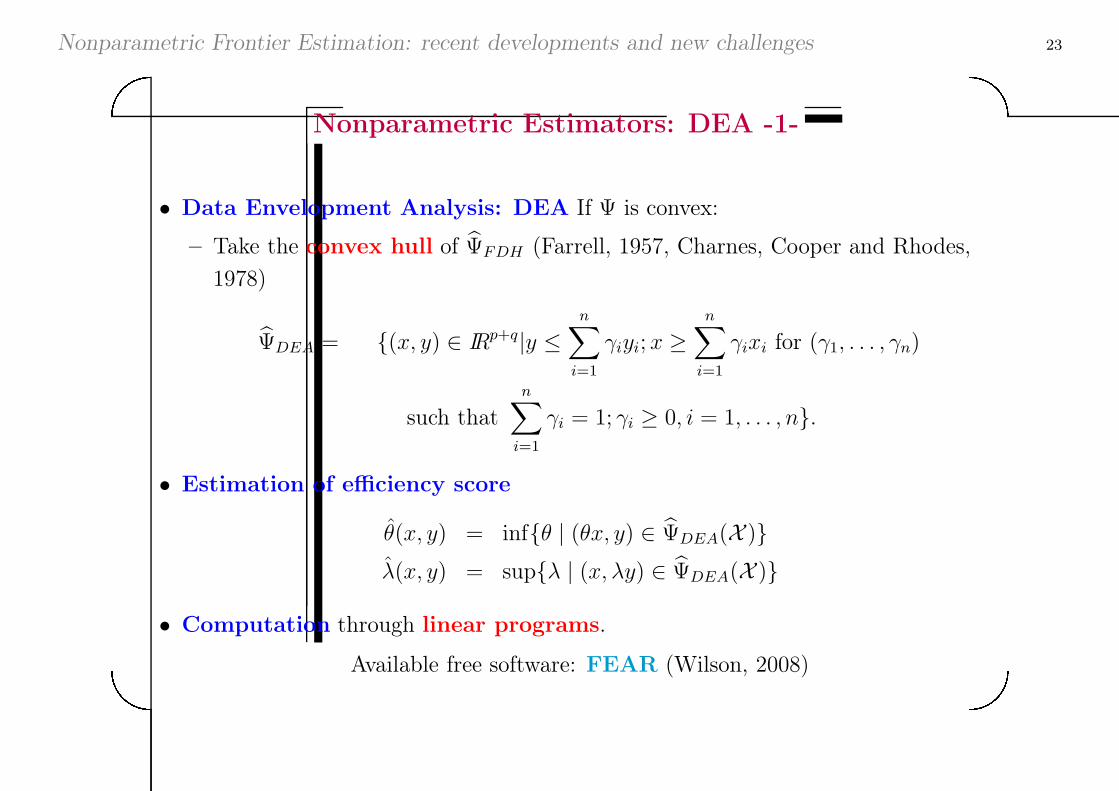
Nonparametric Estimators: DEA -1-
∙ Data Envelopment Analysis: DEA If Ψ is convex:
– Take the convex hull of ΨFDH (Farrell, 1957, Charnes, Cooper and Rhodes,
1978)
ΨDEA = {(x, y) ∈ IRp+q∣y ≤n∑
i=1
iyi; x ≥n∑
i=1
ixi for ( 1, . . . , n)
such that
n∑
i=1
i = 1; i ≥ 0, i = 1, . . . , n}.
∙ Estimation of efficiency score
�(x, y) = inf{� ∣ (�x, y) ∈ ΨDEA(X )}�(x, y) = sup{� ∣ (x, �y) ∈ ΨDEA(X )}
∙ Computation through linear programs.
Available free software: FEAR (Wilson, 2008)
Nonparametric Frontier Estimation: recent developments and new challenges 24'&
$%
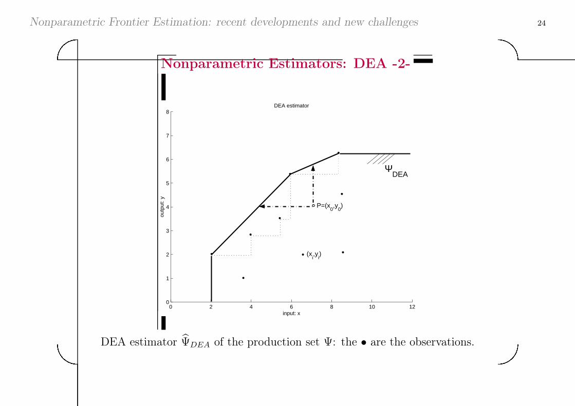
Nonparametric Estimators: DEA -2-
0 2 4 6 8 10 120
1
2
3
4
5
6
7
8
input: x
outp
ut: y
DEA estimator
•
•
•
•
•
•
•
• •
° P=(x0,y
0)
ΨDEA
(xi,y
i)
DEA estimator ΨDEA of the production set Ψ: the ∙ are the observations.
Nonparametric Frontier Estimation: recent developments and new challenges 25'&
$%
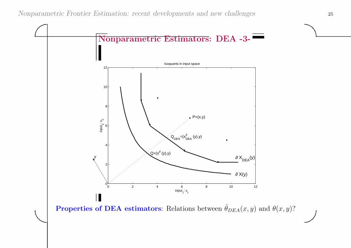
Nonparametric Estimators: DEA -3-
0 2 4 6 8 10 120
2
4
6
8
10
12
input1: x
1
inpu
t 2: x2
Isoquants in input space
•
•
•
•
•
•
•
P=(x,y)
y
QDEA
=(xDEA∂ (y),y)
∂ X(y)
∂ XDEA
(y) Q=(x∂ (y),y)
Properties of DEA estimators: Relations between �DEA(x, y) and �(x, y)?
Nonparametric Frontier Estimation: recent developments and new challenges 26'&
$%
Statistical Inference: State of the Art -1-
Properties: recent survey, Simar and Wilson (2008)
∙ Consistency and rate of convergence:(�(x, y)− �(x, y)
)= Op(n
−�), as n → ∞?
– FDH: Korostelev, Simar and Tsybakov (1995a) and Park, Simar and Weiner
(2000). Rate is n−1/(p+q).
Recent Extensions: Daouia, Florens and Simar (2010)
– DEA: Korostelev, Simar and Tsybakov (1995b) and Kneip, Park and Simar
(1998). Rate is n−2/(p+q+1). Park, Jeong and Simar (2010) (CRS case), rate is
n−2/(p+q).
∙ Nice! but not very useful for the practitionners.
∙ Curse of dimensionality: bad rates if p+ q ↑.
Nonparametric Frontier Estimation: recent developments and new challenges 27'&
$%
Statistical Inference: State of the Art -2-
Is Inference possible ?
∙ Asymptotic sampling distribution:
n�(�(x, y)− �(x, y)
)∼ Q(�), as n → ∞?
– FDH: Park, Simar and Weiner (2000), Badin, Simar (2009), Daouia, Florens
and Simar (2010); Q(�) is a Weibull distribution with unknown
parameters to be estimated: not easy to handle and need large sample sizes if
p+ q increases.
– DEA: Gijbels, Mammen, Park and Simar (1999), Kneip, Simar and Wilson
(2008), Park, Jeong, Simar (2010); Q(�) is a Regular distribution
depending on unknown parameters but no closed forms available (untractable
for practical purposes) when p or q > 1.
∙ No hope ? Yes: the bootstrap.
Nonparametric Frontier Estimation: recent developments and new challenges 28'&
$%
The Bootstrap -1-
Basic Idea
∙ The “Real World” : The Data Generating Process P(xi, yi) in X are realizations of iid random variables (X, Y ) with probability
density function f(x, y) with support Ψ, and Prob((X, Y ) ∈ Ψ
)= 1.
– Ψ(X ) is an estimator of Ψ (FDH or DEA)
– �(x, y) = inf{� ∣ (�x, y) ∈ Ψ(X )} is an estimator of �(x, y)
∙ The “Bootstrap World” : Consider a DGP P , a consistent estimator of P .
We can use Ψ(X ) (FDH or DEA) and some appropriate f(x, y) with support
Ψ(X ), and Prob((X, Y ) ∈ Ψ(X )
)= 1.
∙ Bootstrap Analogy:
Define a new data set X ∗ = {(x∗i , y
∗i ), i = 1, . . . , n} drawn from P .
– Ψ(X ∗) is an estimator of Ψ(X ): here, Ψ(X ∗) is the FDH or DEA set
computed with X ∗ as reference data set.
– �∗(x, y) = inf{� ∣ (�x, y) ∈ Ψ(X ∗)} is an estimator of �(x, y)
Nonparametric Frontier Estimation: recent developments and new challenges 29'&
$%
0 2 4 6 8 10 120
2
4
6
8
10
12
input1: x
1
inpu
t 2: x2
Isoquants in input space
•
•
•
•
•
•
•
P=(x,y)
y
QDEA
∂ X(y)
∂ XDEA
(y)
Q
(xi,y
i)
*
*
*
*
*
Q*DEA
* ∂ X*
DEA(y)
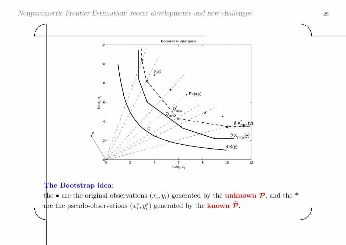
The Bootstrap idea:
the ∙ are the original observations (xi, yi) generated by the unknown 퓟 , and the *
are the pseudo-observations (x∗i , y
∗i ) generated by the known 퓟 .
Nonparametric Frontier Estimation: recent developments and new challenges 30'&
$%
The Bootstrap -2-
∙ The Key Relation : If the Bootstrap is consistent, for large n,
(�∗(x, y)− �(x, y)) ∣ P ≈ (�(x, y)− �(x, y)) ∣ P .
– The right part is unknown and/or difficult to handle
– The left part can be approximated by Monte-Carlo simulation methods
∙ Inference is now available
– Bias correction and Standard errors of �(x, y) are available
– Confidence intervals for �(x, y) can be builded
∙ How to generate X ∗ ? Naive bootstrap looks easy: n random drawns of
(x∗i , y
∗i ) from X .
∙ But naive bootstrap is inconsistent Simar and Wilson (1998, 1999a, 1999b)
– The efficient facet, which determines in the original sample X the value of �,
appears too often, and with a fixed probability, in X ∗ and this fixed
probability does not vanish even when n → ∞.
Nonparametric Frontier Estimation: recent developments and new challenges 31'&
$%
The Bootstrap -3-
Two Solutions: see Simar and Wilson (1998, 2000, 2011a), Jeong and Simar (2006),
Kneip, Simar and Wilson (2008)
∙ Subsampling: draw from P pseudo-samples of size m = n� where � < 1.
– How to chose m in practice: Simar and Wilson (2011a).
∙ Smoothing: Use smoothed density estimate f(x, y) and smooth the boundary
of Ψ when defining P: not easy to implement due to the double smoothing.
– Simplification: homogeneous bootstrap, Simar and Wilson (1998), similar to homoskedastic
assumption in regression. But restrictive. . .
– Consistent efficient algorithm in the heterogeneous case: Kneip, Simar and Wilson (2011).
Testing issues: Returns to scale, Simar and Wilson (2002), Comparison of groups of firms,
Simar and Zelenyuk (2006, 2007), Testing significancy of variables and/or aggregation of variables,
Simar and Wilson (2001), and work in progress (convexity,. . . ).
Extensions available: Hyperbolic distances, Wilson (2011), Directional distances,
Simar and Vanhems (2010), Simar, Vanhems and Wilson (2011).
Nonparametric Frontier Estimation: recent developments and new challenges 32'&
$%
An Example: Program Follow Through (PFT)
∙ Charnes, Cooper, Rhodes (1981): analysis of an experimental education programadministered in US schools: data for 49 schools that implemented PFT, and 21schools that did not, for a total of 70 observations. 5 inputs and 3 outputs
– x1: Education level of the mother (percentage of high school graduates among the mothers),
– x2: Highest occupation of a family member (according a pre-arranged rating scale),
– x3: Parental visit to school index (number of visits to the school)
– x4: Parent counseling index (time spent with child on school related topics)
– x5: Number of teachers of the school.
There are three outputs (results to standard tests):
– y1: Total Reading Score (MAT: Metropolitan Achievement Test),
– y2: Total Mathematics Score (MAT) and
– y3: Coopersmith Self-Esteem Inventory (measure of self-esteem).
∙ We look for output efficiency of the Schools �(x, y) using DEA estimators.
Nonparametric Frontier Estimation: recent developments and new challenges 33'&
$%
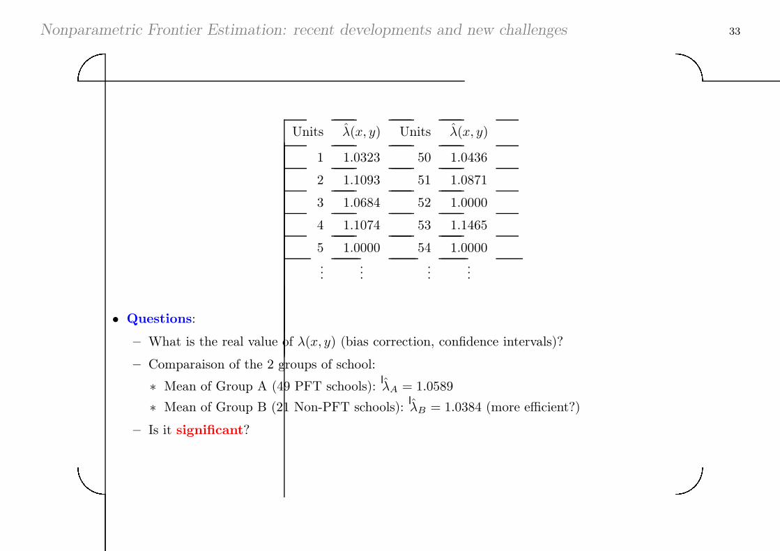
Units �(x, y) Units �(x, y)
1 1.0323 50 1.0436
2 1.1093 51 1.0871
3 1.0684 52 1.0000
4 1.1074 53 1.1465
5 1.0000 54 1.0000...
......
...
∙ Questions:
– What is the real value of �(x, y) (bias correction, confidence intervals)?
– Comparaison of the 2 groups of school:
∗ Mean of Group A (49 PFT schools): �A = 1.0589
∗ Mean of Group B (21 Non-PFT schools): �B = 1.0384 (more efficient?)
– Is it significant?
Nonparametric Frontier Estimation: recent developments and new challenges 34'&
$%
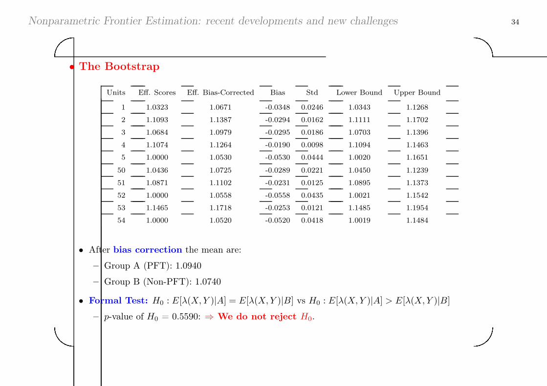
∙ The Bootstrap
Units Eff. Scores Eff. Bias-Corrected Bias Std Lower Bound Upper Bound
1 1.0323 1.0671 -0.0348 0.0246 1.0343 1.1268
2 1.1093 1.1387 -0.0294 0.0162 1.1111 1.1702
3 1.0684 1.0979 -0.0295 0.0186 1.0703 1.1396
4 1.1074 1.1264 -0.0190 0.0098 1.1094 1.1463
5 1.0000 1.0530 -0.0530 0.0444 1.0020 1.1651
50 1.0436 1.0725 -0.0289 0.0221 1.0450 1.1239
51 1.0871 1.1102 -0.0231 0.0125 1.0895 1.1373
52 1.0000 1.0558 -0.0558 0.0435 1.0021 1.1542
53 1.1465 1.1718 -0.0253 0.0121 1.1485 1.1954
54 1.0000 1.0520 -0.0520 0.0418 1.0019 1.1484
∙ After bias correction the mean are:
– Group A (PFT): 1.0940
– Group B (Non-PFT): 1.0740
∙ Formal Test: H0 : E[�(X,Y )∣A] = E[�(X,Y )∣B] vs H0 : E[�(X,Y )∣A] > E[�(X,Y )∣B]
– p-value of H0 = 0.5590: ⇒ We do not reject H0.
Nonparametric Frontier Estimation: recent developments and new challenges 35'&
$%
An Other Example: Role of Innovation on Exports -1-
Schubert and Simar (2011) analyze the relations between exports and innovation in
the sector of “Mechanical Engineering” in Germany (CIS survey, 2007)
∙ The economic literature is unclear and divided on the role of innovation
∙ Empirical studies, so far, used parametric models with restrictive assumptions
and analyze mean behavior of firms (regression)
∙ We want to analyze the role of innovation on efficient production plans, not on
averages
– Data: 215 firms
– 3 inputs: X1 Expenses for personnel, X2 Expenses for equipment and
materials, X3 Expenses for innovation
– 2 outputs: Y1 Domestic turnover et Y2 Exports
Nonparametric Frontier Estimation: recent developments and new challenges 36'&
$%
An Other Example: Role of Innovation on Exports -2-
∙ NB: here individual efficiency scores are not of interest
∙ Results: tests using bootstrap on different models
– The inputs X1 and X2 can be aggregated, without changing the structure of
the efficient frontier, but not X3.
– The outputs Y1 and Y2 can be aggregated
∙ Empirical Conclusions:
– The expenditures in innovation (even measured in monetary terms) are really
different than other routine expenses: they influence the shape of the frontier,
it is really an input, and not a by-product (as claimed by some economic
theory).
– For efficient firms, there is no clear empirical evidence of a link between the
expenses in innovation and the exports (as claimed by some economic theory).
Nonparametric Frontier Estimation: recent developments and new challenges 37'&
$%
IV. Challenges
Nonparametric Frontier Estimation: recent developments and new challenges 38'&
$%
Challenges: Drawbacks of DEA/FDH and Solutions
∙ Sensitivity to extreme/outliers: robust methods and/or detection of outliers
– Order-m frontiers: Cazals, Florens and Simar (2002), Simar (2003), Daouia, Florens and
Simar (2009).
– Order-� quantile frontiers: Aragon, Daouia and Thomas (2005), Daouia and Simar
(2005, 2007), Daouia, Florens and Simar (2009, 2010).
∙ Lack of Economic interpretation: Semiparametric Model, parametric
approximations of nonparametric frontiers, Simar (1992), Florens and Simar (2005), Daouia,
Florens and Simar (2008)
∙ Heterogeneity: How to explain inefficiency by environmental/external factors ?
– Two-stage methods, Simar and Wilson (2007, 2011b).
– Conditional measures of efficiency, Cazals, Florens and Simar (2002), Daraio and
Simar (2005, 2006, 2007a, 2007,b), Jeong, Park and Simar (2010), Badin, Daraio and Simar
(2010, 2011).
∙ No noise is allowed: deterministic frontiers Prob((X,Y ) ∈ Ψ
)= 1: Nonparametric
Stochastic Frontiers?: Simar (2007), Kumbhakar, Park, Simar and Tsionas (2008), Simar
and Zelenyuk, (2011), Kneip, Simar and Van Keilegom (2010), flexible semiparametric models.

Nonparametric Frontier Estimation: recent developments and new challenges 39'&
$%
IV.1 Sensitivity to Outliers
Nonparametric Frontier Estimation: recent developments and new challenges 40'&
$%
Robust Frontier -1
Probabilitic Formulation of DGP
– The DGP: H(x, y) = Prob(X ≤ x, Y ≥ y), Ψ is the support of H(x, y)
– Farrell-Debreu Efficiency score (case of input orientation)
H(x, y) = Prob(X ≤ x ∣Y ≥ y) Prob(Y ≥ y) = FX∣Y (x∣y)SY (y)
�(x0, y0) = inf{�∣(�x0, y0) ∈ Ψ} = inf{�∣FX∣Y (�x0∣y0) > 0}
– Nonparametric Estimator: Plug-in the empirical version of H(x, y)
Hn(x, y) =1
n
n∑
i=1
1I(Xi ≤ x, Yi ≥ y), then FX∣Y,n(x∣y) =Hn(x, y)
Hn(∞, y)
– The FDH estimators: Cazals, Florens and Simar (2002)
– ΨFDH is the support of Hn(x, y)
– Estimation (input) efficiency score: �(x0, y0) = inf{� ∣ FX∣Y,n(�x0∣y0) > 0}
Nonparametric Frontier Estimation: recent developments and new challenges 41'&
$%
Robust Frontier -2-
Partial order frontiers. Economic interpretation (case of univariate output)
Another benchmark frontier less extreme than the “full frontier”.
∙ Order-m: Cazals, Florens, Simar (2002)
– a unit (x, y) is benchmarked against the average maximal output reached by
m peers randomly drawn from the population of units using less input than x.
– As m → ∞, order-m frontier converges to the full-frontier.
∙ Order-� quantile: Aragon, Daouia, Thomas (2005), Daouia and Simar (2007)
– a unit (x, y) is benchmarked against the output level not exceeded by
100(1− �)% of firms in the population of units using less input than x.
– As � → 1, order-� frontier converges to the full-frontier.
Nonparametric Frontier Estimation: recent developments and new challenges 42'&
$%
Robust Frontier -2-
Partial order frontiers: Mathematical definition for univariate output
∙ Full Frontier Benchmark: '(x) = inf{y∣FY ∣X(y∣x) ≥ 1} and
∙ Less Extreme Benchmarks:
– Order-m frontier:
'm(x) = E[max(Y 1, . . . , Y m)∣X ≤ x
]
=
∫ ∞
0
(1− [FY ∣X(y∣x)]m) dy
– Order-� quantile frontier:
'�(x) = F−1Y ∣X(�∣x)
= inf{y ∈ ℝ+∣FY ∣X(y∣x) ≥ �}
Properties
as m → ∞, 'm(x) → '(x) and as � → 1, '�(x) → '(x)
Nonparametric Frontier Estimation: recent developments and new challenges 43'&
$%
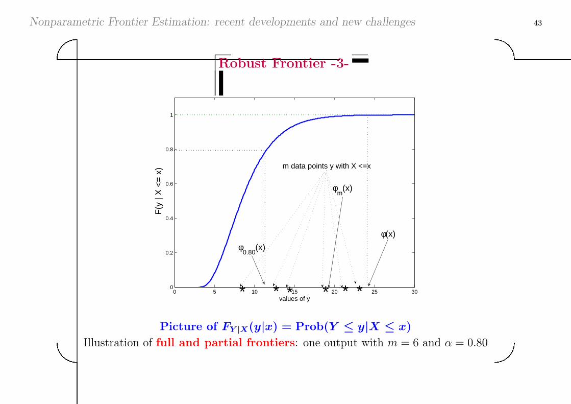
Robust Frontier -3-
0 5 10 15 20 25 300
0.2
0.4
0.6
0.8
1
values of y
F(y
| X
<=
x)
φ(x)
φ0.80
(x)
* * ** * *
m data points y with X <=x
φm
(x)
Picture of FY ∣X(y∣x) = Prob(Y ≤ y∣X ≤ x)
Illustration of full and partial frontiers: one output with m = 6 and � = 0.80
Nonparametric Frontier Estimation: recent developments and new challenges 44'&
$%
Robust Frontier -4-
Nonparametric estimators of partial order frontier
∙ Plug-in principle
'm,n(x) =
∫ ∞
0
(1− [Fn,Y ∣X(y∣x)]m) dy
'�,n(x) = inf{y ∈ ℝ+∣Fn,Y ∣X(y∣x) ≥ �}
∙ Properties
–√n-consistency and asymptotic normality:
√n('m,n(x)− 'm(x))
ℒ−→ N (0, �2m(x)) and
√n('�,n(x)− '�(x))
ℒ−→ N (0, �2�(x))
– Convergence to FDH estimator:
as m → ∞, 'm,n(x) → 'FDH,n(x) and as � → 1, '�,n(x) → 'FDH,n(x)
∙ Choice of m and �: tune the percentage of points left out estimated
partial frontier, see Simar (2003), Daraio, Simar (2005, 2007a).
Nonparametric Frontier Estimation: recent developments and new challenges 45'&
$%
0 0.1 0.2 0.3 0.4 0.5 0.6 0.7 0.8 0.9 10
0.2
0.4
0.6
0.8
1
1.2
1.4
1.6
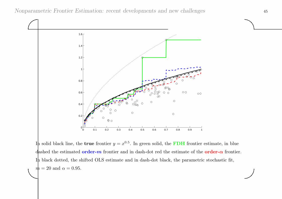
In solid black line, the true frontier y = x0.5. In green solid, the FDH frontier estimate, in blue
dashed the estimated order-m frontier and in dash-dot red the estimate of the order-� frontier.
In black dotted, the shifted OLS estimate and in dash-dot black, the parametric stochastic fit,
m = 20 and � = 0.95.
Nonparametric Frontier Estimation: recent developments and new challenges 46'&
$%
Robust Frontier -5-
Robust Nonparametric Estimator of Full-Frontier '(x), Daouia, Florens,
Simar (2009, 2010)
– If m = m(n) (and � = �(n)) converges to ∞ (to 1) when n → ∞, but at a slow
rate, we obtain an estimator (after bias correction) that converges to the full
frontier with a Normal limiting distribution
– Easy to build confidence intervals for '(x) using Normal Tables.
– For finite n, 'm(n),n(x) and '�(n),n(x) provide estimators of '(x) that will not
envelop all the data points and so, are more robust to extreme and outliers.
Nonparametric Frontier Estimation: recent developments and new challenges 47'&
$%
Robust Frontier -5-
0 500 1000 1500 2000 2500 3000 3500 4000 45000
0.2
0.4
0.6
0.8
1
1.2
1.4
1.6
1.8
2x 10
4
Data pointsFDH frontierphi−tildephi−m
0 500 1000 1500 2000 2500 3000 3500 4000 45000
0.2
0.4
0.6
0.8
1
1.2
1.4
1.6
1.8
2x 10
4
Data pointsFDH frontierphi−tildephi−m
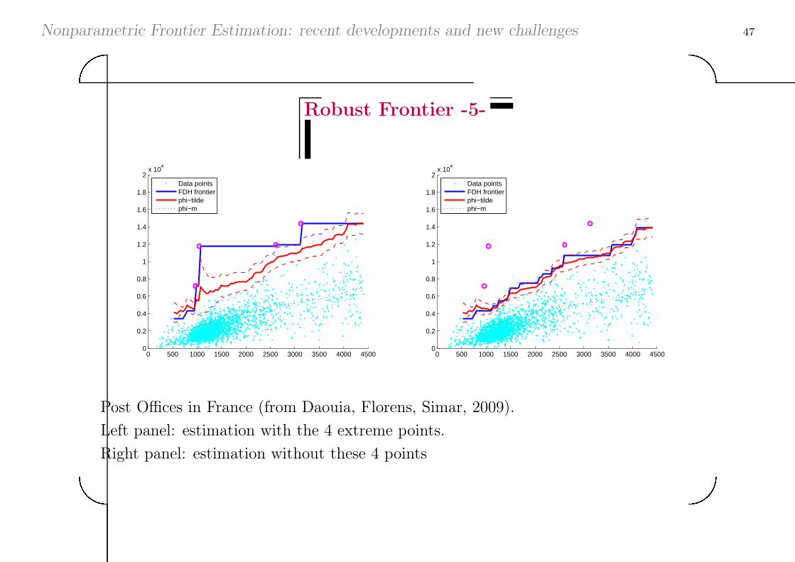
Post Offices in France (from Daouia, Florens, Simar, 2009).
Left panel: estimation with the 4 extreme points.
Right panel: estimation without these 4 points
Nonparametric Frontier Estimation: recent developments and new challenges 48'&
$%
IV.2 Lack of Economic Interpretation
Nonparametric Frontier Estimation: recent developments and new challenges 49'&
$%
Parametric Approximation of Deterministic Frontiers -1-
– Parametric models: easy economic interpretation of the model (returns to
scale, elasticities, elasticities of substitution, . . . )
– Standard parametric approches: some drawbacks
– strong restrictive assumptions on the stochastic part of the models
– sensitive to extreme/outliers
– most are “regression-based” models and capture the shape of the cloud of
points near its center (not at the efficient boundary)
– Two stage semiparametric approaches: Simar (1992), Florens, Simar
(2005), Daouia, Florens, Simar (2008)
– First estimate the efficient frontier using nonparametric or robust
nonparametric methods;
– Then fit, by standard OLS, the approriate parametric model on the
obtained nonparametric frontier
Nonparametric Frontier Estimation: recent developments and new challenges 50'&
$%
Parametric Approximation of Deterministic Frontiers -2-
– More sensible estimator of the parametric frontier model and allows for
some noise by tunning the robustness parameter.
– Asymptotic theory of the resulting estimators (for fix m and fix �):
If FDH is used as 1st step: �np−→ �0
If order-m is used is used as 1st step:√n(�mn − �m0 )
ℒ−→ Nk(0, Vm)
If order-� is used is used as 1st step:√n(��n − ��0 )
ℒ−→ Nk(0, V�)
where �0, (�m0 , ��0 ), are the pseudo-true values of the parameters of the best
approximation of the corresponding frontier '(x), ('m(x), '�(x)).
– If m(n) → ∞ and �(n) → 1 as n → ∞ at appropriate rates:
�na.s.−→ �0 ; �m(n)
na.s.−→ �0 ; ��(n)n
a.s.−→ �0
– Multivariate case: multi-input/muti-output, see Daraio and Simar (2007a)
Nonparametric Frontier Estimation: recent developments and new challenges 51'&
$%
0 0.1 0.2 0.3 0.4 0.5 0.6 0.7 0.8 0.9 10
0.2
0.4
0.6
0.8
1
1.2
1.4
1.6
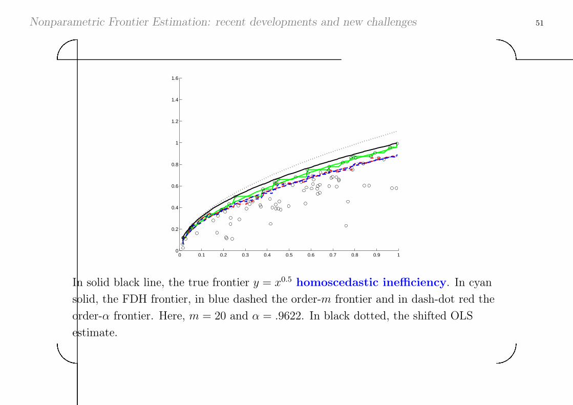
In solid black line, the true frontier y = x0.5 homoscedastic inefficiency. In cyan
solid, the FDH frontier, in blue dashed the order-m frontier and in dash-dot red the
order-� frontier. Here, m = 20 and � = .9622. In black dotted, the shifted OLS
estimate.

Nonparametric Frontier Estimation: recent developments and new challenges 52'&
$%
0 0.1 0.2 0.3 0.4 0.5 0.6 0.7 0.8 0.9 10
0.2
0.4
0.6
0.8
1
1.2
1.4
1.6
Same with 3 outliers included.
Nonparametric Frontier Estimation: recent developments and new challenges 53'&
$%
0 0.1 0.2 0.3 0.4 0.5 0.6 0.7 0.8 0.9 10
0.2
0.4
0.6
0.8
1
1.2
1.4
1.6
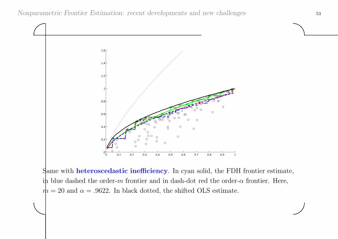
Same with heteroscedastic inefficiency. In cyan solid, the FDH frontier estimate,
in blue dashed the order-m frontier and in dash-dot red the order-� frontier. Here,
m = 20 and � = .9622. In black dotted, the shifted OLS estimate.
Nonparametric Frontier Estimation: recent developments and new challenges 54'&
$%
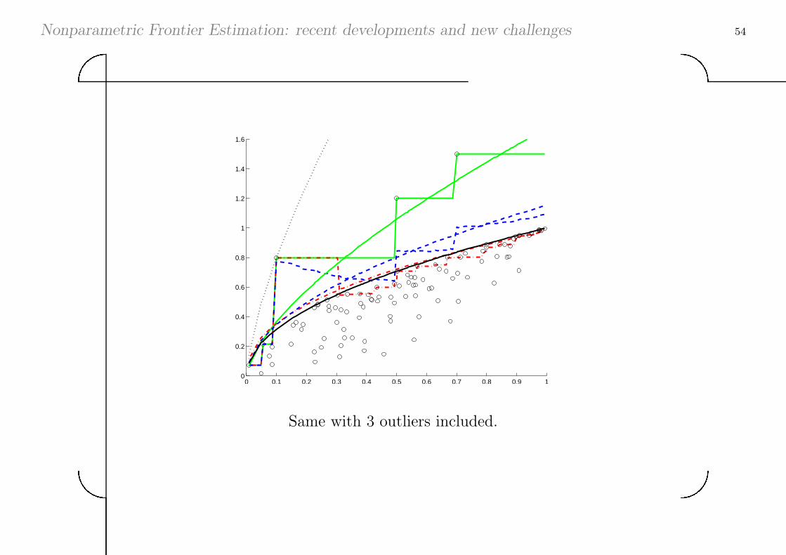
0 0.1 0.2 0.3 0.4 0.5 0.6 0.7 0.8 0.9 10
0.2
0.4
0.6
0.8
1
1.2
1.4
1.6
Same with 3 outliers included.
Nonparametric Frontier Estimation: recent developments and new challenges 55'&
$%
IV.3 Heterogeneity
Nonparametric Frontier Estimation: recent developments and new challenges 56'&
$%
Introducing Environmental Factors -1-
∙ Motivation
– The analysis of productive efficiency should have two components:
1. Estimation of a production frontier (best-practice) which serve as a
benchmark against which efficiency of a producer can be measured;
2. Incorporation into the analysis of exogenous variables (Z) which are
neither inputs, nor outputs, and so are not under the control of the
producer, but which may influence the process.
– How to explain inefficiencies of firms by these factors?
– How to introduce heterogeneity in the production process?
Nonparametric Frontier Estimation: recent developments and new challenges 57'&
$%
Introducing Environmental Factors -2-
∙ One-stage approaches Banker and Morey (1986)
– Z is like an input(favorable) or like an output (defavorable) ⇒ Adapt FDH/DEA
– Free disposability ? Convexity ? RTS assumption ?
– Which direction for Z?
– What if the effect of Z changes?
(say, favorable if Z ≤ z0 and then defavorable or neutral for Z > z0)
∙ Two-stage approaches Simar and Wilson (2007, 2011)
– DEA efficiency scores are regressed on Z (in an appropriate way)
– Implicit Separability Condition:
– Z does not influence Ψ
– Z only affects the probability of being more or less efficient
– The second stage regression is nonstandard (correlation among efficiency
scores, bias,. . . ): inference by bootstrap.
Nonparametric Frontier Estimation: recent developments and new challenges 58'&
$%
Traditional 2-stage approaches
∙ First stage get efficiency estimates �(Xi, Yi) (or �(Xi, Yi), (Xi, Yi),. . . ) with
respect to Ψ (by DEA or FDH, . . . )
∙ Second stage regression of �(Xi, Yi) on Z.
– Parametric models (truncated regression, logistic, etc,. . . )
– Nonparametric models (truncated, etc,. . . )
∙ Problems: Ψz = {(x, y)∣Z = z, x can produce y} Simar and Wilson
(2007, 2011b):
– If Ψz ∕= Ψ, what is the Economic meaning of �(x, y) (and so, of �(Xi, Yi) ),
for a unit facing environmental conditions z?
– Separability issue: condition for giving economic meaning to Ψ and �(x, y).
“Separability” condition: Ψz = Ψ, for all z ∈ 퓩.
– Even if separability holds, Inference in second stage is nonstandard
(bootstrap).
Nonparametric Frontier Estimation: recent developments and new challenges 59'&
$%
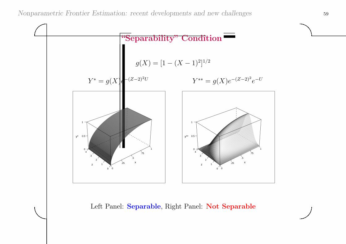
“Separability” Condition
g(X) = [1− (X − 1)2]1/2
Y ∗ = g(X)e−(Z−2)2U Y ∗∗ = g(X)e−(Z−2)2e−U
0
.25
.5
.75
1
0
1
2
3
40
0.5
1
xz
y*
0
.25
.5
.75
1
0
1
2
3
40
0.5
1
xz
y**
Left Panel: Separable, Right Panel: Not Separable
Nonparametric Frontier Estimation: recent developments and new challenges 60'&
$%
Conditional Efficiency -1-
∙ Conditional Measures Cazals, Florens, Simar (2002), Daraio Simar (2005,
2007a, 2007b), Jeong, Park, Simar (2010)
– The DGP (A Model for the Production process) is now characterized by
– F (x, y∣z) = Prob(X ≤ x, Y ≤ y∣Z = z) or
– H(x, y∣z) = Prob(X ≤ x, Y ≥ y∣Z = z)
– The attainable set is Ψz: the support of F (x, y∣z)
– Natural and very easy: A firm combines inputs X ∈ ℝp+ and outputs Y ∈ ℝ
q+
facing the environmental conditions Z ∈ ℝr
– No separability conditions
– No prior information of the role of Z (favorable or not to the process)
– Note that the separability condition of 2-stages methods relies on:
Ψ ≡ Ψz for all z.
Nonparametric Frontier Estimation: recent developments and new challenges 61'&
$%
Conditional Efficiency -2-
∙ Conditional efficiency score
– Same idea as the unconditional measure:
�(x, y∣z) = sup{� ∣ HXY ∣Z(x, �y∣z) > 0} = sup{� ∣ SY ∣X,Z(�y∣x, z) > 0},
where
SY ∣X,Z(y∣x, z) = HXY ∣Z(x, y∣z)/HXY ∣Z(x, 0∣z) = Prob(Y ≥ y ∣ X ≤ x, Z = z).
∙ Nonparametric estimator: kernel smoothing on Z (here continuous)
HXY,n∣Z(x, y∣Z = z) =
∑ni=1 1I(Xi ≤ x, Yi ≥ y)K((Zi − z)/ℎ)∑n
i=1K((Zi − z)/ℎ)
SY ∣X,Z(y∣x, z) =∑n
i=1 1I(Yi ≥ y,Xi ≤ x)Kℎ(Zi, z)∑ni=1 1I(Xi ≤ x)Kℎ(Zi, z)
Nonparametric Frontier Estimation: recent developments and new challenges 62'&
$%
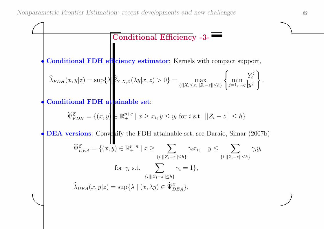
Conditional Efficiency -3-
∙ Conditional FDH efficiency estimator: Kernels with compact support,
�FDH(x, y∣z) = sup{�∣SY ∣X,Z(�y∣x, z) > 0} = max{i∣Xi≤x,∣∣Zi−z∣∣≤ℎ}
{min
j=1,...,q
Y ji
yj
}.
∙ Conditional FDH attainable set:
ΨZFDH = {(x, y) ∈ ℝ
p+q+ ∣ x ≥ xi, y ≤ yi for i s.t. ∣∣Zi − z∣∣ ≤ ℎ}
∙ DEA versions: Convexify the FDH attainable set, see Daraio, Simar (2007b)
ΨZDEA = {(x, y) ∈ ℝ
p+q+ ∣ x ≥
∑
{i∣∣∣Zi−z∣∣≤ℎ}
ixi, y ≤∑
{i∣∣∣Zi−z∣∣≤ℎ}
iyi
for i s.t.∑
{i∣∣∣Zi−z∣∣≤ℎ}
i = 1},
�DEA(x, y∣z) = sup{� ∣ (x, �y) ∈ ΨZDEA}.
Nonparametric Frontier Estimation: recent developments and new challenges 63'&
$%
Conditional Efficiency -4-
∙ Properties
– Optimal bandwidth selection by data-driven methods, Badin, Daraio, Simar
(2010)
– Asymptotic properties: similar to FDH/DEA with n replaced by nℎr, Jeong,
Park, Simar (2010)
– Allow to detect the direction of the “influence” of Z on efficiency, see Dario,
Simar (2005, 2007a)
– Inference (confidence intervals) by bootstrap
– Robust versions (using order-m and order-�) are also available
– Z can be continuous, categorical or discrete
Nonparametric Frontier Estimation: recent developments and new challenges 64'&
$%
Conditional Efficiency -5-
∙ Usefulness
– Define a “pure measure of technical efficiency” , Badin, Daraio, Simar (2011)
– Eliminate most of the influence of Z on �(x, y∣z) by using a flexible
location-scale nonparametric model: �(x, y∣z) = �(z) + �(z)", where �(z) and
�(z) are unspecified functions
– �i allows to rank firms facing different operating conditions.
∙ N.B.: An other approach: Florens, Simar, Van Keilegom (2011).
– First eliminate influence of Z on inputs X and outputs Y by using two flexible
location-scale nonparametric models
– The residuals are “pure inputs and outputs” Xi and Yi
– Search for the frontier in these new units, to define “pure measure of technical
efficiency”
– Full frontier and order-m frontiers
Nonparametric Frontier Estimation: recent developments and new challenges 65'&
$%
Conditional Efficiency, Example -1-
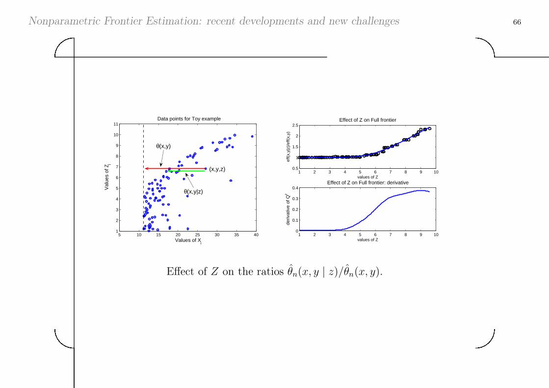
∙ A Toy example:
– No output (Yi ≡ 1) and one input (input orientation)
– Z has no effect on X when Z ≤ 5 and then a defavorable effect on X when
Z > 5.
– The input are generated according
Xi = 51.51I(Zi <= 5) + Z1.5i 1I(Zi > 5) + Ui,
where Zi ∼ U(1, 10), Ui ∼ Expo(� = 3) and n = 100.
Nonparametric Frontier Estimation: recent developments and new challenges 66'&
$%
5 10 15 20 25 30 35 401
2
3
4
5
6
7
8
9
10
11 Data points for Toy example
Values of Xi
Val
ues
of Z
i
θ(x,y)
θ(x,y|z)
(x,y,z) 1 2 3 4 5 6 7 8 9 100.5
1
1.5
2
2.5Effect of Z on Full frontier
values of Z
eff(
x,y|
z)/e
ff(x,
y)
1 2 3 4 5 6 7 8 9 100
0.1
0.2
0.3
0.4Effect of Z on Full frontier: derivative
values of Z
deriv
ativ
e of
Qz
Effect of Z on the ratios �n(x, y ∣ z)/�n(x, y).
Nonparametric Frontier Estimation: recent developments and new challenges 67'&
$%
Conditional Efficiency, Examples -2a-
∙ 2 inputs/ 2 outputs : output orientation
– The efficient frontier is described by: y(2) = 1.0845(x(1))0.3(x(2))0.4 − y(1).
– X(j)i ∼ U(1, 2) and Y
(j)i ∼ U(0.2, 5) for j = 1, 2.
– The output efficient random points on the frontier are
Y(1)i,eff =
1.0845(X(1)i )0.3(X
(2)i )0.4
Si + 1
Y(2)i,eff = 1.0845(X
(1)i )0.3(X
(2)i )0.4 − Y
(1)i,eff .
where Si = Y(2)i /Y
(1)i represent the generated random rays in the output space.
– The efficiencies are simulated according to exp(−Ui)
– The observed output are defined by Yi = Yi,eff ∗ exp(−Ui) where
Ui ∼ Exp(�U = 1/2).
– n = 100.
Nonparametric Frontier Estimation: recent developments and new challenges 68'&
$%
Conditional Efficiency, Examples -2b-
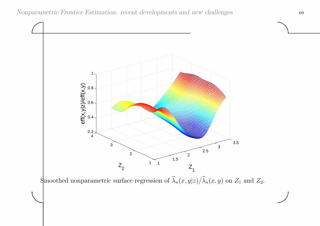
∙ Environmental factors Z bivariate
– We generate two independent uniform variables Zj ∼ U(1, 4) to build the
bivariate variable Z = (Z1, Z2).
– The influence of Z on the production process is described by:
Y(1)i = (1 + 2 ∗ ∣Z1 − 2.5∣3) ∗ Y (1)
i,eff ∗ exp(−Ui)
Y(2)i = (1 + 2 ∗ ∣Z1 − 2.5∣3) ∗ Y (2)
i,eff ∗ exp(−Ui).
– Z1 pushes the efficient frontier above when far from 2.5, in both directions,
with a cubic effect,
– Z2 has no effect on the frontier or on the distribution of inefficiencies: Z2 is
irrelevant.
– Note that there is no interaction between Z1 and Z2 (independent) and no
interaction between X and Z.
– Remember: only n = 100 observations, with p = q = r = 2 !
Nonparametric Frontier Estimation: recent developments and new challenges 69'&
$%
11.5
22.5
33.5
1
2
3
40.2
0.4
0.6
0.8
1
Z1
Z2
eff(
x,y|
z)/e
ff(x,
y)
Smoothed nonparametric surface regression of �n(x, y∣z)/�n(x, y) on Z1 and Z2.
Nonparametric Frontier Estimation: recent developments and new challenges 70'&
$%
1.5 2 2.5 30
0.5
1
Effect of Z1 on Full frontier
values of Z1
eff(
x,y|
z)/e
ff(x,
y)
1.5 2 2.5 3 3.50
0.5
1
Effect of Z2 on Full frontier
values of Z2
eff(
x,y|
z)/e
ff(x,
y)
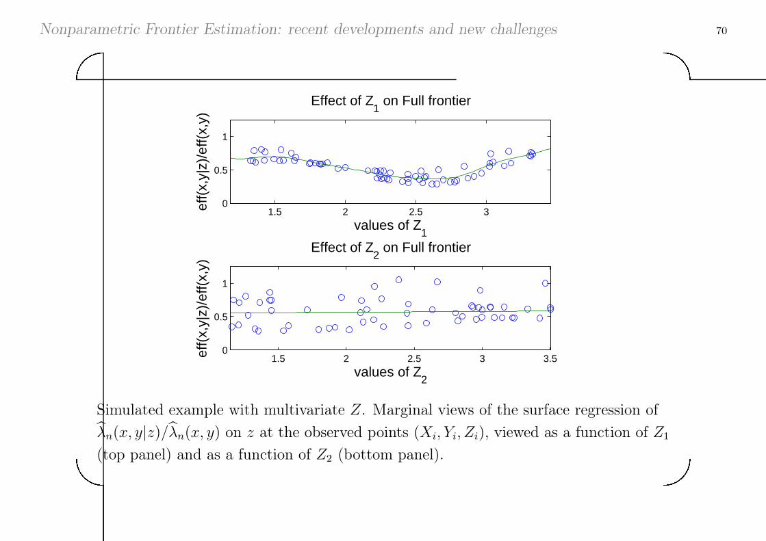
Simulated example with multivariate Z. Marginal views of the surface regression of
�n(x, y∣z)/�n(x, y) on z at the observed points (Xi, Yi, Zi), viewed as a function of Z1
(top panel) and as a function of Z2 (bottom panel).
Nonparametric Frontier Estimation: recent developments and new challenges 71'&
$%
IV.4 Introducing Noise
Nonparametric Frontier Estimation: recent developments and new challenges 72'&
$%
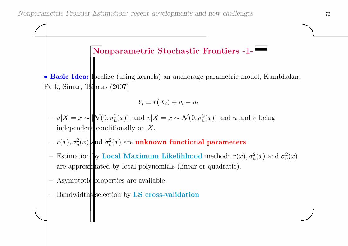
Nonparametric Stochastic Frontiers -1-
∙ Basic Idea: localize (using kernels) an anchorage parametric model, Kumbhakar,
Park, Simar, Tsionas (2007)
Yi = r(Xi) + vi − ui
– u∣X = x ∼ ∣N (0, �2u(x))∣ and v∣X = x ∼ N (0, �2
v(x)) and u and v being
independent conditionally on X.
– r(x), �2u(x) and �2
v(x) are unknown functional parameters
– Estimation by Local Maximum Likelihhood method: r(x), �2u(x) and �2
v(x)
are approximated by local polynomials (linear or quadratic).
– Asymptotic properties are available
– Bandwidths selection by LS cross-validation
Nonparametric Frontier Estimation: recent developments and new challenges 73'&
$%
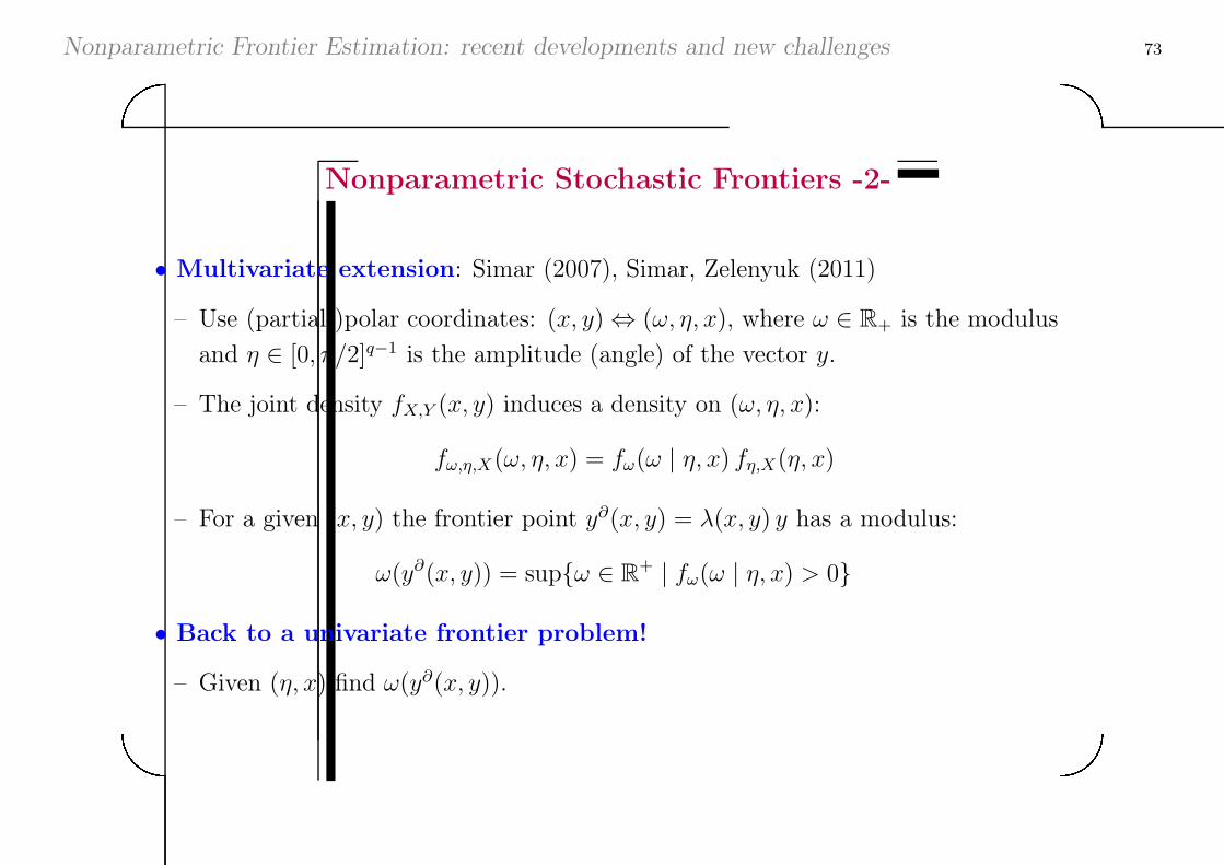
Nonparametric Stochastic Frontiers -2-
∙ Multivariate extension: Simar (2007), Simar, Zelenyuk (2011)
– Use (partial-)polar coordinates: (x, y) ⇔ (!, �, x), where ! ∈ ℝ+ is the modulus
and � ∈ [0, �/2]q−1 is the amplitude (angle) of the vector y.
– The joint density fX,Y (x, y) induces a density on (!, �, x):
f!,�,X(!, �, x) = f!(! ∣ �, x) f�,X(�, x)
– For a given (x, y) the frontier point y∂(x, y) = �(x, y) y has a modulus:
!(y∂(x, y)) = sup{! ∈ ℝ+ ∣ f!(! ∣ �, x) > 0}
∙ Back to a univariate frontier problem!
– Given (�, x) find !(y∂(x, y)).
Nonparametric Frontier Estimation: recent developments and new challenges 74'&
$%
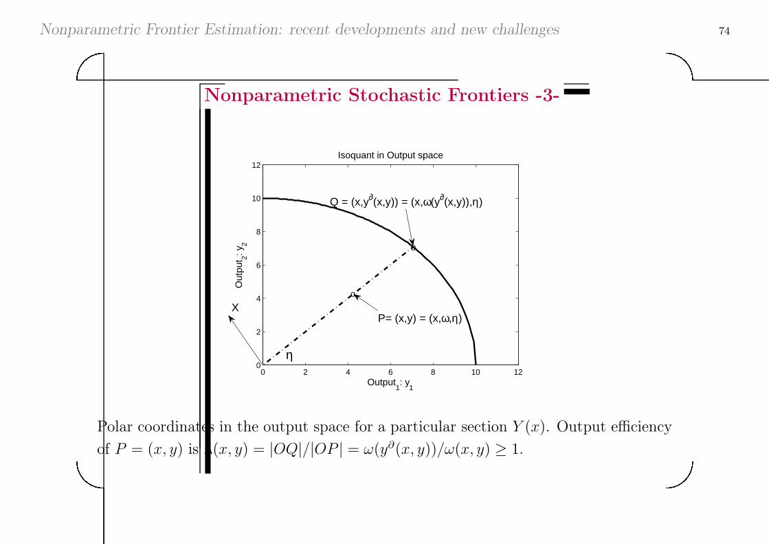
Nonparametric Stochastic Frontiers -3-
0 2 4 6 8 10 120
2
4
6
8
10
12Isoquant in Output space
Output1: y
1
Out
put 2: y
2
XP= (x,y) = (x,ω,η)
o
Q = (x,y∂(x,y)) = (x,ω(y∂(x,y)),η)
o
η
Polar coordinates in the output space for a particular section Y (x). Output efficiency
of P = (x, y) is �(x, y) = ∣OQ∣/∣OP ∣ = !(y∂(x, y))/!(x, y) ≥ 1.
Nonparametric Frontier Estimation: recent developments and new challenges 75'&
$%
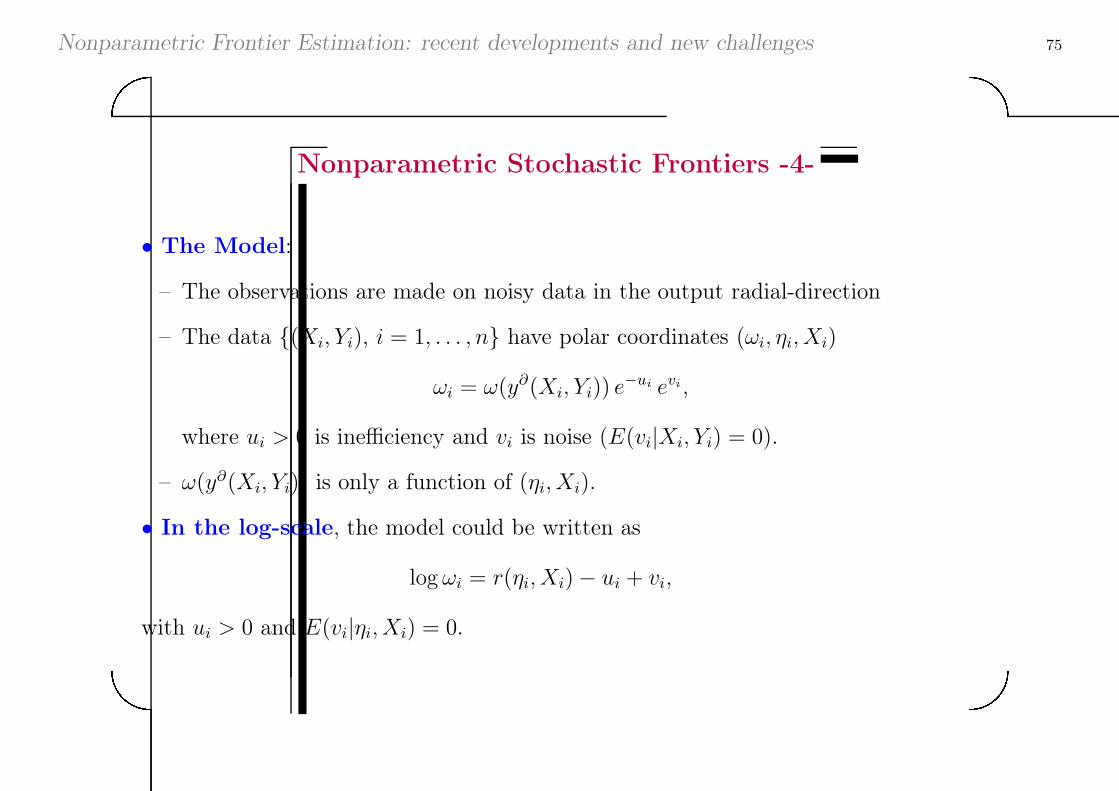
Nonparametric Stochastic Frontiers -4-
∙ The Model:
– The observations are made on noisy data in the output radial-direction
– The data {(Xi, Yi), i = 1, . . . , n} have polar coordinates (!i, �i, Xi)
!i = !(y∂(Xi, Yi)) e−ui evi ,
where ui > 0 is inefficiency and vi is noise (E(vi∣Xi, Yi) = 0).
– !(y∂(Xi, Yi)) is only a function of (�i, Xi).
∙ In the log-scale, the model could be written as
log!i = r(�i, Xi)− ui + vi,
with ui > 0 and E(vi∣�i, Xi) = 0.
Nonparametric Frontier Estimation: recent developments and new challenges 76'&
$%
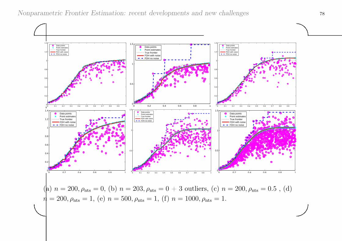
Nonparametric Stochastic Frontiers -5-
– Stochastic Versions of DEA/FDH : Two-stage procedure
– [1] “Whitening the noise”: Compute the consistent estimator of the frontier
levels r(�i, Xi) for each data points
∗ This gives points (Xi, Y∗i ) where Y ∗
i = exp(r(�i, Xi))Yi/!i
– [2] Run a DEA (or FDH) program with reference set (Xi, Y∗i ).
– Summary:
– Very encouraging results
– Computationally demanding (cross-validation for bandwidth selection)
– Below, some bivariate examples (see multivariate examples in Simar and
Zelenyuk, 2011)
Nonparametric Frontier Estimation: recent developments and new challenges 77'&
$%
0 0.1 0.2 0.3 0.4 0.5 0.6 0.7 0.8 0.9 10.1
0.2
0.3
0.4
0.5
0.6
0.7
0.8
0.9
1
1.1
Data pointsPoint estimatesTrue frontierDEA with noiseDEA no noise
0 0.2 0.4 0.6 0.8 10
0.2
0.4
0.6
0.8
1
1.2
1.4Data pointsPoint estimatesTrue frontierDEA with noiseDEA no noise
0 0.2 0.4 0.6 0.8 10
0.2
0.4
0.6
0.8
1
1.2
1.4Data pointsPoint estimatesTrue frontierDEA with noiseDEA no noise
0 0.1 0.2 0.3 0.4 0.5 0.6 0.7 0.8 0.9 10
0.2
0.4
0.6
0.8
1
1.2
1.4
Data pointsPoint estimatesTrue frontierDEA with noiseDEA no noise
0 0.1 0.2 0.3 0.4 0.5 0.6 0.7 0.8 0.9 10
0.2
0.4
0.6
0.8
1
1.2
1.4
Data pointsPoint estimatesTrue frontierDEA with noiseDEA no noise
0 0.1 0.2 0.3 0.4 0.5 0.6 0.7 0.8 0.9 10
0.5
1
1.5
2
2.5
Data pointsPoint estimatesTrue frontierDEA with noiseDEA no noise
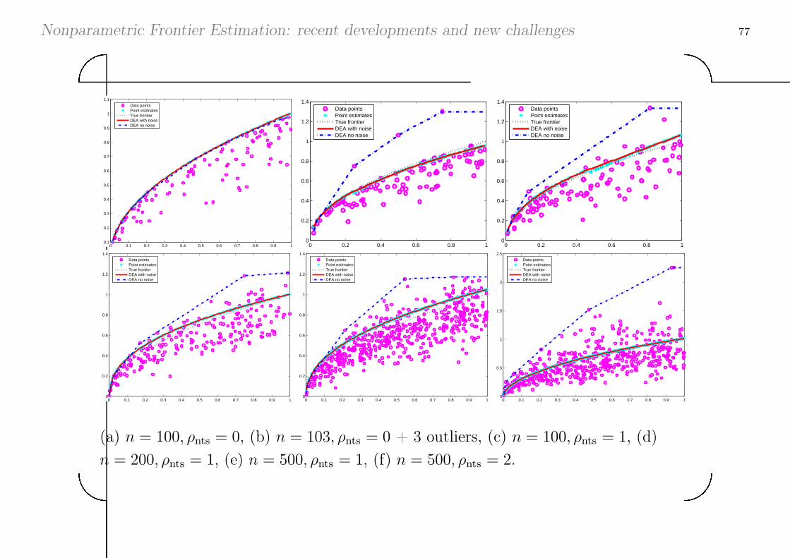
(a) n = 100, �nts = 0, (b) n = 103, �nts = 0 + 3 outliers, (c) n = 100, �nts = 1, (d)
n = 200, �nts = 1, (e) n = 500, �nts = 1, (f) n = 500, �nts = 2.
Nonparametric Frontier Estimation: recent developments and new challenges 78'&
$%
0 0.1 0.2 0.3 0.4 0.5 0.6 0.7 0.8 0.9 10
0.2
0.4
0.6
0.8
1
1.2
1.4
Data pointsPoint estimatesTrue frontierFDH with noiseFDH no noise
0 0.2 0.4 0.6 0.8 10
0.5
1
1.5Data pointsPoint estimatesTrue frontierFDH with noiseFDH no noise
0 0.1 0.2 0.3 0.4 0.5 0.6 0.7 0.8 0.9 10
0.2
0.4
0.6
0.8
1
1.2
1.4
Data pointsPoint estimatesTrue frontierFDH with noiseFDH no noise
0 0.2 0.4 0.6 0.8 10
0.2
0.4
0.6
0.8
1
1.2
1.4Data pointsPoint estimatesTrue frontierFDH with noiseFDH no noise
0 0.1 0.2 0.3 0.4 0.5 0.6 0.7 0.8 0.9 10
0.5
1
1.5
Data pointsPoint estimatesTrue frontierFDH with noiseFDH no noise
0 0.2 0.4 0.6 0.8 10
0.5
1
1.5Data pointsPoint estimatesTrue frontierFDH with noiseFDH no noise
(a) n = 200, �nts = 0, (b) n = 203, �nts = 0 + 3 outliers, (c) n = 200, �nts = 0.5 , (d)
n = 200, �nts = 1, (e) n = 500, �nts = 1, (f) n = 1000, �nts = 1.
Nonparametric Frontier Estimation: recent developments and new challenges 79'&
$%
Conclusions
∙ Nonparametric models NP are Econometric Models
– Flexible and can be “robustified”, Inference is available (bootstrap)
– Noise can be introduced
– Environmental factors (heterogeneity) can be introduced
∙ P and NP are complimentary models
– NP models can be used to check (test) P models (not the contrary).
– Parametric approximations of NP models can be useful for economic analysis.
– Semiparametric models should be developed.
∙ Other challenges
– Panel Data: introduce dynamic behavior of units
– Theory for functions of DEA/FDH scores: Kneip, Simar and Wilson (2011)
∗ Useful for justifying testing procedures
∗ RTS, Convexity, Simar and Wilson (2011a), Separabilty, Daraio, Simar and
Wilson (2010),. . .
Nonparametric Frontier Estimation: recent developments and new challenges 80'&
$%
References
∙ Basic References
– Fried, H., Lovell, K. and S. Schmidt (eds) (2008),The Measurement of
Productive Efficiency, 2nd Edition, Oxford University Press.
– Kumbhakar, S.C. and C.A.K. Lovell (2000), Stochastic Frontier Analysis,
Cambridge University Press.
– Daraio, C. and L. Simar (2007a), Advanced Robust and Nonparametric
Methods in Efficiency Analysis. Methodology and Applications, Springer,
New-York.
– Simar, L. and P.W. Wilson (2008), Statistical Inference in Nonparametric
Frontier Models: recent Developments and Perspectives, in The Measurement
of Productive Efficiency, 2nd Edition, Harold Fried, C.A.Knox Lovell and
Shelton Schmidt, editors, Oxford University Press, 2008.
Nonparametric Frontier Estimation: recent developments and new challenges 81'&
$%
∙ References list
∙ Aigner, D.J., Lovell, C.A.K. and P. Schmidt (1977), Formulation and estimation of stochastic
frontier models, Journal of Econometrics, 6, 21-37.
∙ Aragon, Y. and Daouia, A. and Thomas-Agnan, C. (2005), Nonparametric Frontier
Estimation: A Conditional Quantile-based Approach, Econometric Theory, 21, 358–389.
∙ Badin, M., Daraio, C. and L. Simar (2010), Optimal Bandwidth Selection for Conditional
Efficiency Measures: a Data-driven Approach, European Journal of Operational Research, 201,
633–640
∙ Badin, L., Daraio, C. and L. Simar (2011), How to measure the impact of environmental factors
in a nonparametric production model? Discussion paper 2011/19, Institut de Statistique, UCL.
∙ Badin, L. and L. Simar (2009), A bias corrected nonparametric envelopment estimator of
frontiers, Econometric Theory, 25, 5, 1289–1318.
∙ Banker, R.D. and R.C. Morey (1986), Efficiency analysis for exogenously fixed inputs and
outputs, Operations Research, 34(4), 513–521.
∙ Cazals, C. Florens, J.P. and L. Simar (2002), Nonparametric Frontier Estimation: a Robust
Approach , in Journal of Econometrics, 106, 1–25.
∙ Chambers, R. G., Y. Chung, and R. Färe (1998), Profit, directional distance functions, and
nerlovian efficiency, Journal of Optimization Theory and Applications, 98, 351–364.
Nonparametric Frontier Estimation: recent developments and new challenges 82'&
$%
∙ Charnes, A., Cooper W.W. and E. Rhodes (1978), Measuring the inefficiency of decision
making units, European Journal of Operational Research 2 (6), 429-444.
∙ Daouia, A., J.P. Florens and L. Simar (2008), Functional Convergence of Quantile-type
Frontiers with Application to Parametric Approximations, Journal of Statistical Planning and
Inference, 138, 708–725.
∙ Daouia, A., Florens, J.P. and L. Simar (2009), Regularization of Non-parametric Frontier
Estimators. Discussion paper 0922, Institut de Statistique, UCL.
∙ Daouia, A., Florens, J.P. and L. Simar (2010), Frontier estimation and extreme values theory.
Bernoulli, 16(4), 1039–1063.
∙ Daouia, A. and L. Simar (2005), Robust Nonparametric Estimators of Monotone Boundaries,
Journal of Multivariate Analysis, 96, 311–331.
∙ Daouia, A. and L. Simar (2007), Nonparametric efficiency analysis: a multivariate conditional
quantile approach, Journal of Econometrics, 140, 375–400.
∙ Daraio, C. and L. Simar (2005), Introducing environmental variables in nonparametric frontier
models: a probabilistic approach, Journal of Productivity Analysis, vol 24, 1, 93–121.
∙ Daraio, C. and L. Simar (2006), A Robust Nonparametric Approach to Evaluate and Explain
the Performance of Mutual Funds, European Journal of Operational Research, vol 175, 1,
516–542.
Nonparametric Frontier Estimation: recent developments and new challenges 83'&
$%
∙ Daraio, C. and L. Simar (2007a), Advanced Robust and Nonparametric Methods in Efficiency
Analysis. Methodology and Applications, Springer, New-York.
∙ Daraio, C. and L. Simar (2007), Conditional nonparametric frontier models for convex and non
convex technologies: a unifying approach, Journal of Productivity Analysis, vol 28, 13–32.
∙ Daraio, C., Simar, L. and P.W. Wilson (2010), Testing whether Two-Stage Estimation is
Meaningful in Non-Parametric Models of Production, Discussion paper 1031, Institut de
Statistique, UCL.
∙ Debreu, G. (1951), The coefficient of ressource utilization, Econometrica, 19:3, 273-292.
∙ Deprins, D., Simar, L. and H. Tulkens (1984), Measuring labor inefficiency in post offices. In
The Performance of Public Enterprises: Concepts and measurements . M. Marchand, P.
Pestieau and H. Tulkens (eds.), Amsterdam, North-Holland, 243–267.
∙ Farrell, M.J. (1957), The measurement of productive efficiency. Journal of the Royal Statistical
Society, Series A, 120, 253–281.
∙ Färe, R. and S. Grosskopf (2000), Theory and application of directional distance functions,
Journal of Productivity Analysis 13, 93–103.
∙ Färe, R., and S. Grosskopf (2004), New Directions: Efficiency and Productivity, Boston:
Kluwer Academic Publishers.
∙ Färe, R., S. Grosskopf, and C. A. K. Lovell (1985), The Measurement of Efficiency of
Production, Boston: Kluwer-Nijhoff Publishing.
Nonparametric Frontier Estimation: recent developments and new challenges 84'&
$%
∙ Florens, J.P. and L. Simar, (2005), Parametric Approximations of Nonparametric Frontier,
Journal of Econometrics, vol 124, 1, 91–116
∙ Fried, H., Lovell, K. and S. Schmidt (eds) (2008),The Measurement of Productive Efficiency,
2nd Edition, Oxford University Press.
∙ Gijbels, I., E. Mammen, B.U. Park and L. Simar (1999), On Estimation of Monotone and
Concave Frontier Functions, Journal of the American Statistical Association, vol 94, 445,
220-228.
∙ Hall, P. and L. Simar (2002), Estimating a Changepoint, Boundary or Frontier in the Presence
of Observation Error, Journal of the American Statistical Association, 97, 523–534.
∙ Jeong, S.O. , B. U. Park and L. Simar (2010), Nonparametric conditional efficiency measures:
asymptotic properties. Annals of Operations Research, 173, 105–122.
∙ Jeong, S.O. and L. Simar (2006), Linearly interpolated FDH efficiency score for nonconvex
frontiers, Journal of Multivariate Analysis, 97, 2141–2161.
∙ Kneip, A., Park, B.U. and Simar, L. (1998). : A note on the convergence of nonparametric
DEA estimators for production efficiency scores. Econometric Theory, 14, 783–793.
∙ Kneip, A., Simar, L. and I. Van Keilegom (2010), Boundary Estimation in the Presence of
Measurement Errors. Discussion paper 1046, Institut de Statistique, UCL.
∙ Kneip, A, L. Simar and P.W. Wilson (2008), Asymptotics and consistent bootstraps for DEA
estimators in non-parametric frontier models, Econometric Theory, 24, 1663–1697.
Nonparametric Frontier Estimation: recent developments and new challenges 85'&
$%
∙ Kneip, A., Simar, L. and P.W. Wilson (2011), A Computational Efficient, Consistent Bootstrap
for Inference with Non-parametric DEA Estimators. Discussion paper 0903, Institut de
Statistique, UCL, in press Computational Economics.
∙ Kneip, A., Simar, L. and P.W. Wilson (2011), Central Limit Theorems for DEA efficiency
scores: when bias can kill the variance. Discussion paper 2011/**, Institut de Statistique, UCL.
∙ Koopmans, T.C.(1951), An analysis of production as an efficient combination of activities, in
Koopmans, T.C. (ed) Activity Analysis of Production and Allocation, Cowles Commision for
Research in Economics, Monograph 13, John-Wiley, New-York.
∙ Korostelev, A., Simar, L. and A. Tsybakov (1995a), Efficient Estimation of Monotone
Boundaries, Annals of Statistics, 23(2), 476–489.
∙ Korostelev, A., Simar, L. and A. Tsybakov (1995b), On Estimation of Monotone and Convex
Boundaries, Publications des Instituts de Statistique des Universités de Paris, 1, 3–18.
∙ Kumbhakar, S.C. and C.A.K. Lovell (2000), Stochastic Frontier Analysis, Cambridge
University Press.
∙ Kumbhakar, S.C. , Park, B.U., Simar, L. and E.G. Tsionas (2007), Nonparametric stochastic
frontiers: a local likelihood approach, Journal of Econometrics, 137, 1, 1–27.
∙ Mouchart, M. and L. Simar (2002), Efficiency analysis of Air Controlers: first insights,
Consulting report 0202, Institut de Statistique, Université Catholique de Louvain, Belgium.
Nonparametric Frontier Estimation: recent developments and new challenges 86'&
$%
∙ Park, B.U., Jeong, S.-O. and L. Simar (2010), Asymptotic Distribution of Conical-Hull
Estimators of Directional Edges. Annals of Statistics, Vol 38, 6, 1320–1340.
∙ Park, B. Simar, L. and Ch. Weiner (2000), The FDH Estimator for Productivity Efficiency
Scores: Asymptotic Properties, Econometric Theory, Vol 16, 855–877.
∙ Park, B., L. Simar and V. Zelenyuk (2008), Local Likelihood Estimation of Truncated
Regression and its Partial Derivatives: Theory and Application, Journal of Econometrics, 146,
185–198.
∙ Ritter, C. and L. Simar (1997), Pitfalls of normal-gamma stochastic frontier models, Journal of
Productivity Analysis, 8, 167–182.
∙ Schubert, T. and L. Simar (2011), Innovation and export activities in the German mechanical
engineering sector: an application of testing restrictions in production analysis. Journal of
Productivity Analysis, 36, 55–69.
∙ Shephard, R.W. (1970). Theory of Cost and Production Function. Princeton University Press,
Princeton, New-Jersey.
∙ Simar, L. (1992), Estimating efficiencies from frontier models with panel data: a comparison of
parametric, non-parametric and semi-parametric methods with bootstrapping, Journal of
Productivity Analysis, 3, 167-203.
Nonparametric Frontier Estimation: recent developments and new challenges 87'&
$%
∙ Simar, L. (2003), Detecting Outliers in Frontiers Models: a Simple Approach, Journal of
Productivity Analysis, 20, 391–424.
∙ Simar, L. (2007), How to Improve the Performances of DEA/FDH Estimators in the Presence
of Noise, Journal of Productivity Analysis, vol 28, 183–201.
∙ Simar, L. and A. Vanhems (2010), Probabilist Characterization of Directional Distances and
their Robust versions. Discussion paper 1040, Institut de Statistique, UCL, to appear Journal
of Econometrics.
∙ Simar, L., Vanhems, A. and P.W. Wilson (2011), Statistical inference with DEA estimators of
directional distances. Discussion paper 2011/**, Institut de Statistique, UCL.
∙ Simar, L. and P. Wilson (1998), Sensitivity of efficiency scores : How to bootstrap in
Nonparametric frontier models, Management Sciences, 44, 1, 49–61.
∙ Simar, L. and P. Wilson (1999a), Some problems with the Ferrier/Hirschberg Bootstrap Idea,
Journal of Productivity Analysis, 11, 67–80.
∙ Simar, L. and P. Wilson (1999b), Of Course we can bootstrap DEA scores ! But does it mean
anything ? Logic trumps wishful thinking, Journal of Productivity Analysis, 11, 93–97.
∙ Simar L. and P. Wilson (2000), A General Methodology for Bootstrapping in Nonparametric
Frontier Models, Journal of Applied Statistics, Vol 27, 6, 779–802.
Nonparametric Frontier Estimation: recent developments and new challenges 88'&
$%
∙ Simar L. and P. Wilson (2001), Testing Restrictions in Nonparametric Efficiency Models,
Communications in Statistics, simulation and computation, 30 (1), 159–184.
∙ Simar L. and P. Wilson (2002), Nonparametric Test of Return to Scale, European Journal of
Operational Research, 139, 115–132.
∙ Simar, L and P. Wilson (2007), Estimation and Inference in Two-Stage, Semi-Parametric
Models of Production Processes, Journal of Econometrics, vol 136, 1, 31–64.
∙ Simar, L. and P.W. Wilson (2008), Statistical Inference in Nonparametric Frontier Models:
recent Developments and Perspectives, in The Measurement of Productive Efficiency, 2nd
Edition, Harold Fried, C.A.Knox Lovell and Shelton Schmidt, editors, Oxford University Press,
2008.
∙ Simar, L. and P.W. Wilson (2010), Inference From Cross-Sectional Stochastic Frontier Models.
Econometric Review, 29, 1, 62–98.
∙ Simar, L. and P.W. Wilson (2011a), Inference by the m out of n bootstrap in nonparametric
frontier models. Journal of Productivity Analysis, 36, 33–53.
∙ Simar, L. and P.W. Wilson (2011b), Two-Stage DEA: Caveat Emptor. Discussion paper 1041,
Institut de Statistique, UCL, in press Journal of Productivity Analysis.
Nonparametric Frontier Estimation: recent developments and new challenges 89'&
$%
∙ Simar, L. and V. Zelenyuk (2006), On Testing Equality of Two Distribution Functions of
Efficiency Score Estimated via DEA, Econometric Review, 25(4), 497-522.
∙ Simar, L. and V. Zelenyuk (2007), Statistical Inference for Aggregates of Farrell-type
Efficiencies, Journal of Applied Econometrics, vol 22, 7, 1367–1394.
∙ Simar, L. and V. Zelenyuk (2011), Stochastic FDH/DEA estimators for frontier analysis.
Journal of Productivity Analysis, 36, 1–20..
∙ Wilson, P.W. (2008), FEAR 1.0: A Software Package for Frontier Efficiency Analysis with R,
Socio-Economic Planning Sciences 42, 247–254.
∙ Wilson, P.W. (2011), Asymptotic properties of some non-parametric hyperbolic efficiency
estimators, in I. van Keilegom and P. W. Wilson, eds., Exploring Research Frontiers in
Contemporary Statistics and Econometrics, Berlin: Springer-Verlag.