NonlinearControl Lecture#6 Passivity and Input-OutputStabilitykhalil/NonlinearControl/... ·...

Nonlinear Control

Lecture # 6

Passivity

and

Input-Output Stability

Nonlinear Control Lecture # 6 Passivity and Input-Output Stability

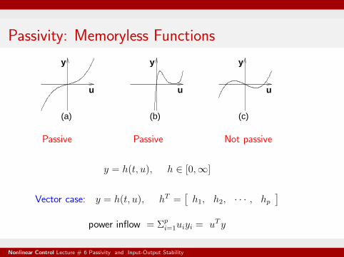
Passivity: Memoryless Functions

u

y

(a)

u

y

(b)

u

y

(c)

Passive Passive Not passive

y = h(t, u), h ∈ [0,∞]

Vector case: y = h(t, u), hT =[

h1, h2, · · · , hp]

power inflow = Σpi=1uiyi = uTy


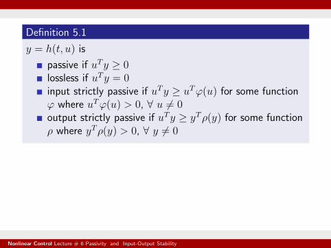
Definition 5.1

y = h(t, u) is

passive if uTy ≥ 0lossless if uTy = 0input strictly passive if uTy ≥ uTϕ(u) for some functionϕ where uTϕ(u) > 0, ∀ u 6= 0output strictly passive if uTy ≥ yTρ(y) for some functionρ where yTρ(y) > 0, ∀ y 6= 0


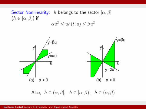
Sector Nonlinearity: h belongs to the sector [α, β](h ∈ [α, β]) if

αu2 ≤ uh(t, u) ≤ βu2

y=αu

y= uβ

u

(a)

y

α > 0

y=αu

y=β

u

y

(b)

u

α < 0

Also, h ∈ (α, β], h ∈ [α, β), h ∈ (α, β)


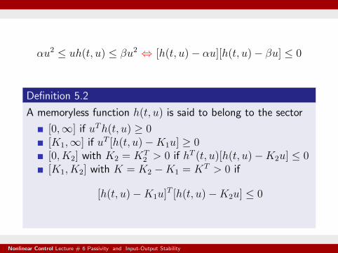
αu2 ≤ uh(t, u) ≤ βu2 ⇔ [h(t, u)− αu][h(t, u)− βu] ≤ 0

Definition 5.2

A memoryless function h(t, u) is said to belong to the sector

[0,∞] if uTh(t, u) ≥ 0[K1,∞] if uT [h(t, u)−K1u] ≥ 0[0, K2] with K2 = KT

2 > 0 if hT (t, u)[h(t, u)−K2u] ≤ 0[K1, K2] with K = K2 −K1 = KT > 0 if

[h(t, u)−K1u]T [h(t, u)−K2u] ≤ 0


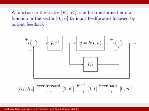
A function in the sector [K1, K2] can be transformed into afunction in the sector [0,∞] by input feedforward followed byoutput feedback

✲✍✌✎☞

✲ K−1 ✲ y = h(t, u) ✲✍✌✎☞

✲

✲ K1

✻✻

+

+

+

−

[K1, K2]Feedforward

−→ [0, K]K−1

−→ [0, I]Feedback

−→ [0,∞]


Passivity: State Models

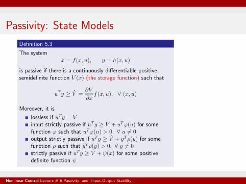
Definition 5.3

The systemx = f(x, u), y = h(x, u)

is passive if there is a continuously differentiable positivesemidefinite function V (x) (the storage function) such that

uTy ≥ V =∂V

∂xf(x, u), ∀ (x, u)

Moreover, it is

lossless if uTy = Vinput strictly passive if uTy ≥ V + uTϕ(u) for somefunction ϕ such that uTϕ(u) > 0, ∀ u 6= 0output strictly passive if uTy ≥ V + yTρ(y) for somefunction ρ such that yTρ(y) > 0, ∀ y 6= 0strictly passive if uTy ≥ V + ψ(x) for some positivedefinite function ψ


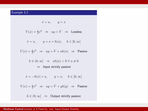
Example 5.2

x = u, y = x

V (x) = 12x2 ⇒ uy = V ⇒ Lossless

x = u, y = x+ h(u), h ∈ [0,∞]

V (x) = 12x2 ⇒ uy = V + uh(u) ⇒ Passive

h ∈ (0,∞] ⇒ uh(u) > 0 ∀ u 6= 0

⇒ Input strictly passive

x = −h(x) + u, y = x, h ∈ [0,∞]

V (x) = 12x2 ⇒ uy = V + yh(y) ⇒ Passive

h ∈ (0,∞] ⇒ Output strictly passive


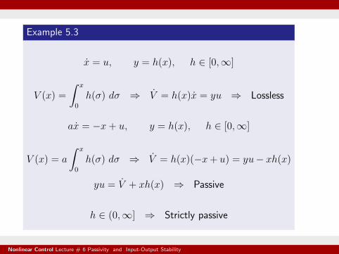
Example 5.3

x = u, y = h(x), h ∈ [0,∞]

V (x) =

∫ x

0

h(σ) dσ ⇒ V = h(x)x = yu ⇒ Lossless

ax = −x+ u, y = h(x), h ∈ [0,∞]

V (x) = a

∫ x

0

h(σ) dσ ⇒ V = h(x)(−x+ u) = yu− xh(x)

yu = V + xh(x) ⇒ Passive

h ∈ (0,∞] ⇒ Strictly passive


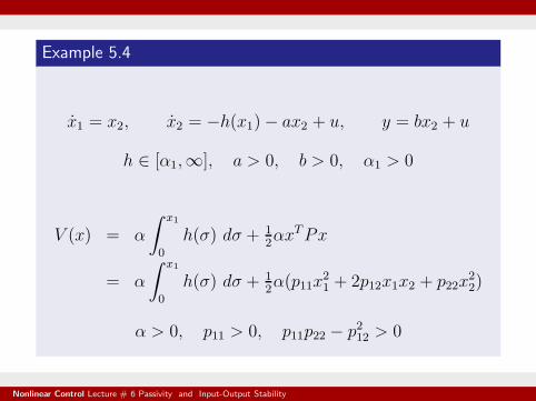
Example 5.4

x1 = x2, x2 = −h(x1)− ax2 + u, y = bx2 + u

h ∈ [α1,∞], a > 0, b > 0, α1 > 0

V (x) = α

∫ x1

0

h(σ) dσ + 12αxTPx

= α

∫ x1

0

h(σ) dσ + 12α(p11x

21 + 2p12x1x2 + p22x

22)

α > 0, p11 > 0, p11p22 − p212 > 0


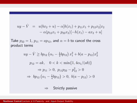
uy − V = u(bx2 + u)− α[h(x1) + p11x1 + p12x2]x2

− α(p12x1 + p22x2)[−h(x1)− ax2 + u]

Take p22 = 1, p11 = ap12, and α = b to cancel the crossproduct terms

uy − V ≥ bp12(

α1 − 14bp12

)

x21 + b(a− p12)x22

p12 = ak, 0 < k < min{1, 4α1/(ab)}⇒ p11 > 0, p11p22 − p212 > 0

⇒ bp12(

α1 − 14bp12

)

> 0, b(a− p12) > 0

⇒ Strictly passive


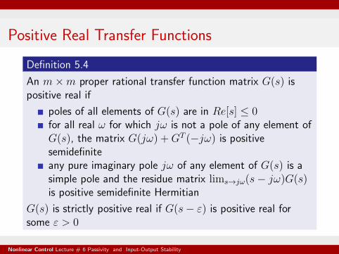
Positive Real Transfer Functions

Definition 5.4

An m×m proper rational transfer function matrix G(s) ispositive real if

poles of all elements of G(s) are in Re[s] ≤ 0for all real ω for which jω is not a pole of any element ofG(s), the matrix G(jω) +GT (−jω) is positivesemidefiniteany pure imaginary pole jω of any element of G(s) is asimple pole and the residue matrix lims→jω(s− jω)G(s)is positive semidefinite Hermitian

G(s) is strictly positive real if G(s− ε) is positive real forsome ε > 0


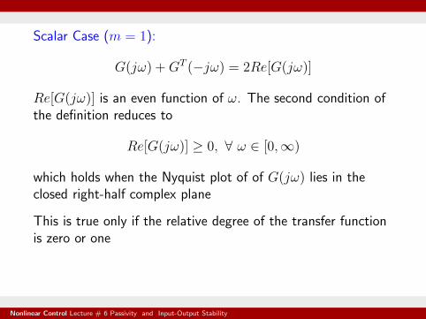
Scalar Case (m = 1):

G(jω) +GT (−jω) = 2Re[G(jω)]

Re[G(jω)] is an even function of ω. The second condition ofthe definition reduces to

Re[G(jω)] ≥ 0, ∀ ω ∈ [0,∞)

which holds when the Nyquist plot of of G(jω) lies in theclosed right-half complex plane

This is true only if the relative degree of the transfer functionis zero or one


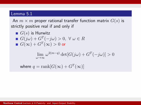
Lemma 5.1

An m×m proper rational transfer function matrix G(s) isstrictly positive real if and only if

G(s) is HurwitzG(jω) +GT (−jω) > 0, ∀ ω ∈ RG(∞) +GT (∞) > 0 or

limω→∞

ω2(m−q) det[G(jω) +GT (−jω)] > 0

where q = rank[G(∞) +GT (∞)]


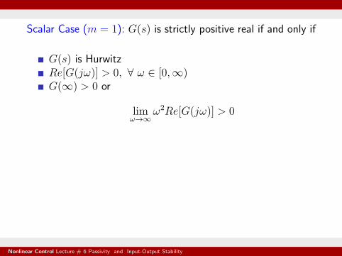
Scalar Case (m = 1): G(s) is strictly positive real if and only if

G(s) is HurwitzRe[G(jω)] > 0, ∀ ω ∈ [0,∞)G(∞) > 0 or

limω→∞

ω2Re[G(jω)] > 0


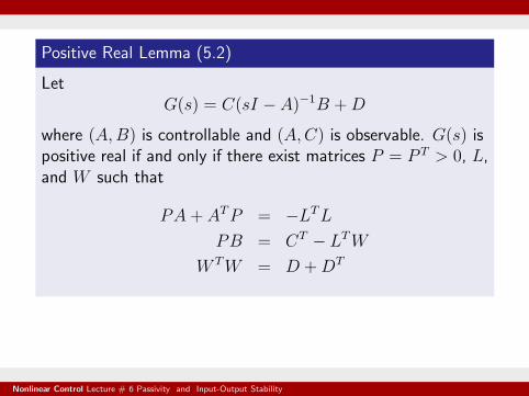
Positive Real Lemma (5.2)

LetG(s) = C(sI −A)−1B +D

where (A,B) is controllable and (A,C) is observable. G(s) ispositive real if and only if there exist matrices P = P T > 0, L,and W such that

PA+ ATP = −LTL

PB = CT − LTW

W TW = D +DT


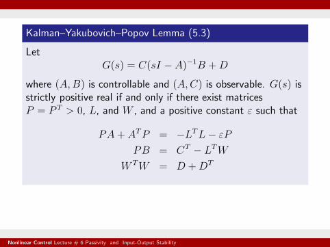
Kalman–Yakubovich–Popov Lemma (5.3)

LetG(s) = C(sI −A)−1B +D

where (A,B) is controllable and (A,C) is observable. G(s) isstrictly positive real if and only if there exist matricesP = P T > 0, L, and W , and a positive constant ε such that

PA+ ATP = −LTL− εP

PB = CT − LTW

W TW = D +DT


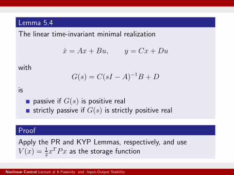
Lemma 5.4

The linear time-invariant minimal realization

x = Ax+Bu, y = Cx+Du

withG(s) = C(sI −A)−1B +D

is

passive if G(s) is positive realstrictly passive if G(s) is strictly positive real

Proof

Apply the PR and KYP Lemmas, respectively, and useV (x) = 1

2xTPx as the storage function


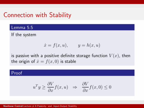
Connection with Stability

Lemma 5.5

If the system

x = f(x, u), y = h(x, u)

is passive with a positive definite storage function V (x), thenthe origin of x = f(x, 0) is stable

Proof

uTy ≥ ∂V

∂xf(x, u) ⇒ ∂V

∂xf(x, 0) ≤ 0


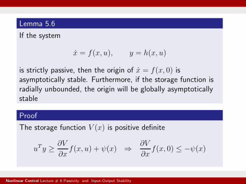
Lemma 5.6

If the system

x = f(x, u), y = h(x, u)

is strictly passive, then the origin of x = f(x, 0) isasymptotically stable. Furthermore, if the storage function isradially unbounded, the origin will be globally asymptoticallystable

Proof

The storage function V (x) is positive definite

uTy ≥ ∂V

∂xf(x, u) + ψ(x) ⇒ ∂V

∂xf(x, 0) ≤ −ψ(x)


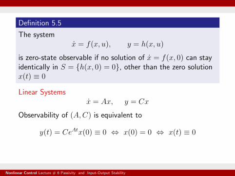
Definition 5.5

The systemx = f(x, u), y = h(x, u)

is zero-state observable if no solution of x = f(x, 0) can stayidentically in S = {h(x, 0) = 0}, other than the zero solutionx(t) ≡ 0

Linear Systemsx = Ax, y = Cx

Observability of (A,C) is equivalent to

y(t) = CeAtx(0) ≡ 0 ⇔ x(0) = 0 ⇔ x(t) ≡ 0


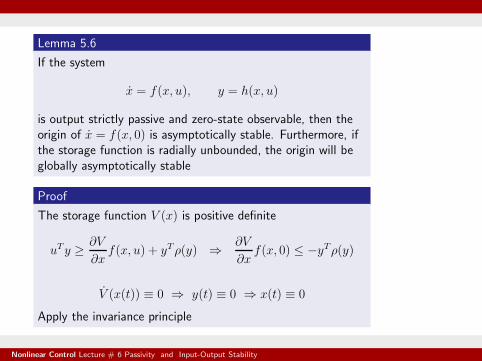
Lemma 5.6

If the system

x = f(x, u), y = h(x, u)

is output strictly passive and zero-state observable, then theorigin of x = f(x, 0) is asymptotically stable. Furthermore, ifthe storage function is radially unbounded, the origin will beglobally asymptotically stable

Proof

The storage function V (x) is positive definite

uTy ≥ ∂V

∂xf(x, u) + yTρ(y) ⇒ ∂V

∂xf(x, 0) ≤ −yTρ(y)

V (x(t)) ≡ 0 ⇒ y(t) ≡ 0 ⇒ x(t) ≡ 0

Apply the invariance principle


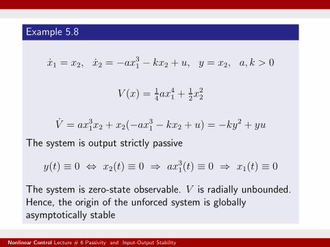
Example 5.8

x1 = x2, x2 = −ax31 − kx2 + u, y = x2, a, k > 0

V (x) = 14ax41 +

12x22

V = ax31x2 + x2(−ax31 − kx2 + u) = −ky2 + yu

The system is output strictly passive

y(t) ≡ 0 ⇔ x2(t) ≡ 0 ⇒ ax31(t) ≡ 0 ⇒ x1(t) ≡ 0

The system is zero-state observable. V is radially unbounded.Hence, the origin of the unforced system is globallyasymptotically stable


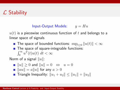
L Stability

Input-Output Models: y = Hu

u(t) is a piecewise continuous function of t and belongs to alinear space of signals

The space of bounded functions: supt≥0 ‖u(t)‖ <∞The space of square-integrable functions:∫∞

0uT (t)u(t) dt <∞

Norm of a signal ‖u‖:‖u‖ ≥ 0 and ‖u‖ = 0 ⇔ u = 0‖au‖ = a‖u‖ for any a > 0Triangle Inequality: ‖u1 + u2‖ ≤ ‖u1‖+ ‖u2‖


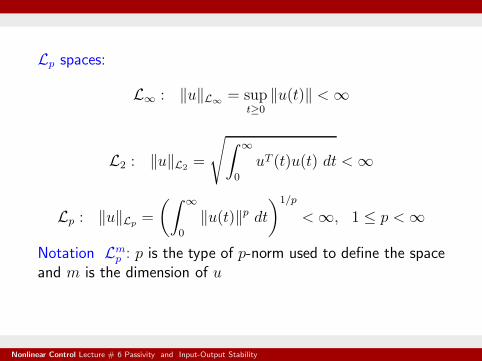
Lp spaces:

L∞ : ‖u‖L∞= sup

t≥0‖u(t)‖ <∞

L2 : ‖u‖L2=

√

∫ ∞

0

uT (t)u(t) dt <∞

Lp : ‖u‖Lp=

(∫ ∞

0

‖u(t)‖p dt)1/p

<∞, 1 ≤ p <∞

Notation Lmp : p is the type of p-norm used to define the space

and m is the dimension of u


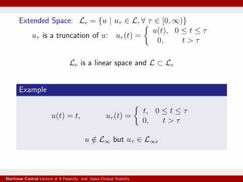
Extended Space: Le = {u | uτ ∈ L, ∀ τ ∈ [0,∞)}uτ is a truncation of u: uτ(t) =

{

u(t), 0 ≤ t ≤ τ0, t > τ

Le is a linear space and L ⊂ Le

Example

u(t) = t, uτ(t) =

{

t, 0 ≤ t ≤ τ0, t > τ

u /∈ L∞ but uτ ∈ L∞e


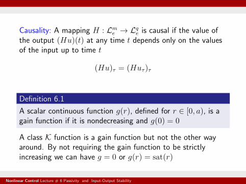
Causality: A mapping H : Lme → Lq

e is causal if the value ofthe output (Hu)(t) at any time t depends only on the valuesof the input up to time t

(Hu)τ = (Huτ)τ

Definition 6.1

A scalar continuous function g(r), defined for r ∈ [0, a), is again function if it is nondecreasing and g(0) = 0

A class K function is a gain function but not the other wayaround. By not requiring the gain function to be strictlyincreasing we can have g = 0 or g(r) = sat(r)


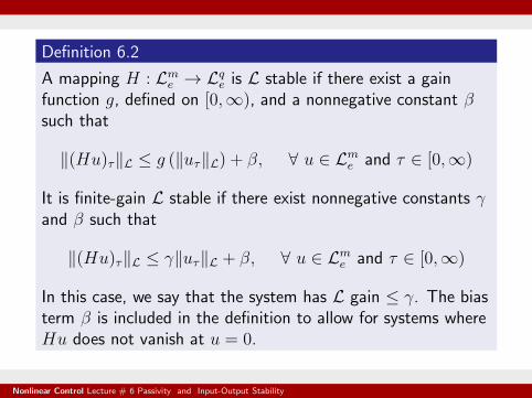
Definition 6.2

A mapping H : Lme → Lq

e is L stable if there exist a gainfunction g, defined on [0,∞), and a nonnegative constant βsuch that

‖(Hu)τ‖L ≤ g (‖uτ‖L) + β, ∀ u ∈ Lme and τ ∈ [0,∞)

It is finite-gain L stable if there exist nonnegative constants γand β such that

‖(Hu)τ‖L ≤ γ‖uτ‖L + β, ∀ u ∈ Lme and τ ∈ [0,∞)

In this case, we say that the system has L gain ≤ γ. The biasterm β is included in the definition to allow for systems whereHu does not vanish at u = 0.


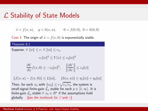
L Stability of State Models

x = f(x, u), y = h(x, u), 0 = f(0, 0), 0 = h(0, 0)

Case 1: The origin of x = f(x, 0) is exponentially stable

Theorem 6.1

Suppose, ∀ ‖x‖ ≤ r, ∀ ‖u‖ ≤ ru,

c1‖x‖2 ≤ V (x) ≤ c2‖x‖2

∂V

∂xf(x, 0) ≤ −c3‖x‖2,

∥

∥

∥

∥

∂V

∂x

∥

∥

∥

∥

≤ c4‖x‖

‖f(x, u)− f(x, 0)‖ ≤ L‖u‖, ‖h(x, u)‖ ≤ η1‖x‖+ η2‖u‖Then, for each x0 with ‖x0‖ ≤ r

√

c1/c2, the system issmall-signal finite-gain Lp stable for each p ∈ [1,∞]. It isfinite-gain Lp stable ∀ x0 ∈ Rn if the assumptions holdglobally [see the textbook for β and γ]


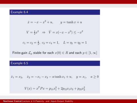
Example 6.4

x = −x− x3 + u, y = tanh x+ u

V = 12x2 ⇒ V = x(−x − x3) ≤ −x2

c1 = c2 =12, c3 = c4 = 1, L = η1 = η2 = 1

Finite-gain Lp stable for each x(0) ∈ R and each p ∈ [1,∞]

Example 6.5

x1 = x2, x2 = −x1 − x2 − a tanh x1 + u, y = x1, a ≥ 0

V (x) = xTPx = p11x21 + 2p12x1x2 + p22x

22


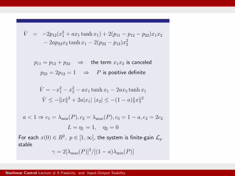
V = −2p12(x21 + ax1 tanh x1) + 2(p11 − p12 − p22)x1x2

− 2ap22x2 tanh x1 − 2(p22 − p12)x22

p11 = p12 + p22 ⇒ the term x1x2 is canceled

p22 = 2p12 = 1 ⇒ P is positive definite

V = −x21 − x22 − ax1 tanh x1 − 2ax2 tanh x1

V ≤ −‖x‖2 + 2a|x1| |x2| ≤ −(1− a)‖x‖2

a < 1 ⇒ c1 = λmin(P ), c2 = λmax(P ), c3 = 1− a, c4 = 2c2

L = η1 = 1, η2 = 0

For each x(0) ∈ R2, p ∈ [1,∞], the system is finite-gain Lp

stableγ = 2[λmax(P )]

2/[(1− a)λmin(P )]


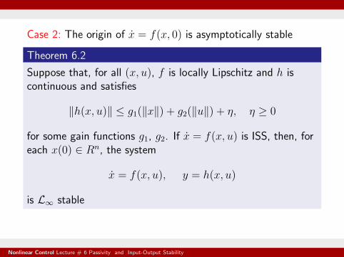
Case 2: The origin of x = f(x, 0) is asymptotically stable

Theorem 6.2

Suppose that, for all (x, u), f is locally Lipschitz and h iscontinuous and satisfies

‖h(x, u)‖ ≤ g1(‖x‖) + g2(‖u‖) + η, η ≥ 0

for some gain functions g1, g2. If x = f(x, u) is ISS, then, foreach x(0) ∈ Rn, the system

x = f(x, u), y = h(x, u)

is L∞ stable


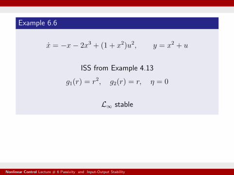
Example 6.6

x = −x− 2x3 + (1 + x2)u2, y = x2 + u

ISS from Example 4.13

g1(r) = r2, g2(r) = r, η = 0

L∞ stable


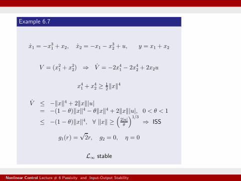
Example 6.7

x1 = −x31 + x2, x2 = −x1 − x32 + u, y = x1 + x2

V = (x21 + x22) ⇒ V = −2x41 − 2x42 + 2x2u

x41 + x42 ≥ 12‖x‖4

V ≤ −‖x‖4 + 2‖x‖|u|= −(1 − θ)‖x‖4 − θ‖x‖4 + 2‖x‖|u|, 0 < θ < 1

≤ −(1 − θ)‖x‖4, ∀ ‖x‖ ≥(

2|u|θ

)1/3

⇒ ISS

g1(r) =√2r, g2 = 0, η = 0

L∞ stable


NonlinearControl Lecture#6 Passivity and Input-OutputStabilitykhalil/NonlinearControl/... ·...

Documents

Transcript of NonlinearControl Lecture#6 Passivity and Input-OutputStabilitykhalil/NonlinearControl/... ·...