7th International Conference on Ocean Energy 2018 // Cherbourg, France

1

New Mechanical Features for Time-Domain WEC

Modelling in InWave

David Ogden*#1, Remy Pascal *, Adrien Combourieu**, David Forehandφ, Lars Johanningχ, Zhi-Ming Yuanψ

*Innosea Ltd., Edinburgh, UK #Industrial Doctoral Centre for Offshore Renewable Energy (IDCORE)

1email: david.ogden@innosea.fr **Innosea SAS, Nantes, France

φInstitute for Energy Systems, University of Edinburgh, Edinburgh, UK χCollege of Engineering, Mathematics and Physical Sciences, University of Exeter, Penryn, UK

ψDepartment of Naval Architecture, Ocean and Marine Engineering, University of Strathclyde, Glasgow, UK

Abstract- Numerical modelling of wave energy converters

(WECs) can provide insights into device performance at an

early stage and help de-risk projects before progressing to

more advanced, costlier stages of development. Several

software packages have been made available for this purpose

in recent years. However, the lack of design convergence in

the wave energy industry, with its wide range of working

principles and mechanisms, means that many developers have

been unable use these tools. Here we show that some

limitations can be overcome by using an alternative

multibody dynamics approach. A third party multibody

dynamics code based on the Lagrange multiplier method,

Hotint, has been coupled to Innosea’s existing WEC

modelling code, InWave, and verified using existing test

cases. This has made the modelling of many new types of

mechanisms possible – include closed mechanical loops.

Keywords- InWave, Multibody Dynamics, WEC Simulation

I. INTRODUCTION

A well-known characteristic of the wave energy industry is

the lack of design convergence among WECs. Indeed, despite

the industry developing 8 different categories of WEC, all

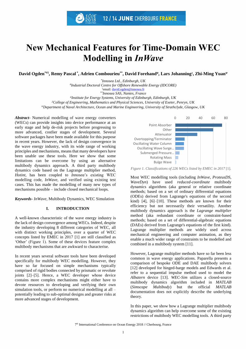
with distinct working principles, over a quarter of WEC

concepts listed by EMEC in 2017 [1] are still classified as

‘Other’ (Figure 1). Some of these devices feature complex

multibody mechanisms that are awkward to characterise.

In recent years several software tools have been developed

specifically for multibody WEC modelling. However, they

have so far focused on simple mechanisms typically

comprised of rigid bodies connected by prismatic or revolute

joints [2]–[5]. Hence, a WEC developer whose device

contains more complex mechanisms might either have to

devote resources to developing and verifying their own

simulation tools, or perform no numerical modelling at all –

potentially leading to sub-optimal designs and greater risks at

more advanced stages of development.

Figure 1. Classifications of 226 WECs listed by EMEC in 2017 [1].

Most WEC modelling tools (including InWave, ProteusDS,

WaveDyn) have used reduced-coordinate multibody

dynamics algorithms (aka general or relative coordinate

methods; based on a set of ordinary differential equations

(ODEs) derived from Lagrange's equations of the second

kind) [4], [6]–[10]. These methods are known for their

efficiency but not necessarily their versatility. Another

multibody dynamics approach is the Lagrange multiplier

method (aka redundant coordinate or constraint-based

methods; based on a set of differential-algebraic equations

(DAEs) derived from Lagrange's equations of the first kind).

Lagrange multiplier methods are widely used across

mechanical engineering and computer animation, as they

enable a much wider range of constraints to be modelled and

combined in a multibody system [11].

However, Lagrange multiplier methods have so far been less

common in wave energy applications. Paparella presents a

comparison of bespoke ODE and DAE multibody solvers

[12] developed for hinged-barge models and Edwards et al.

refer to a sequential impulse method used to model the

Albatern device [13]. WEC-Sim utilizes a closed-source

multibody dynamics algorithm included in MATLAB

(Simscape Multibody) but the official MATLAB

documentation does not explicitly describe the underlying

theory.

In this paper, we show how a Lagrange multiplier multibody

dynamics algorithm can help overcome some of the existing

restrictions of multibody WEC modelling tools. A third party

0 20 40 60 80

Bulge WaveRotating Mass

Submerged Pressure…Oscillating Wave Surge…

Oscillating Water ColumnOvertopping/Terminator

AttenuatorOther

Point Absorber

7th International Conference on Ocean Energy 2018 // Cherbourg, France

2

multibody dynamics code based on the Lagrange multiplier

method, Hotint, has been coupled to Innosea’s existing

multibody WEC modelling tool, InWave. To distinguish the

new developments from the original InWave code, we refer

to it as InWave+H. Verification of InWave+H is presented,

and a demonstration of some of the new capabilities (e.g.

closed mechanical loops) is also shown.

II. THEORY & METHODOLOGY

Here we present the underlying theory of the Lagrange

multiplier method and show how it can incorporate fluid

mechanics for WEC modelling. One of the main objectives of

the Lagrange multiplier method is to determine the constraint

force vector - 𝑱𝑇𝜆, and include it in the system’s equations of

motion:

𝑴�̇⃗⃗� = 𝑱𝑇𝜆 + 𝑓𝑒𝑥𝑡

Where 𝑓𝑒𝑥𝑡 contains all of the external forces acting on the

system. For an 𝑛-body system,

𝑴 = [

𝑴1 𝟎𝟎 𝑴2

⋯ 𝟎 ⋯ 𝟎

⋮ ⋮𝟎 𝟎

⋱ ⋮⋯ 𝑴𝑛

] , �⃗⃗� = [

�⃗⃗�1

�⃗⃗�2

⋮�⃗⃗�𝑛

] , 𝑓𝑒𝑥𝑡 =

[ 𝑓1

𝑓2

⋮

𝑓𝑛]

An important difference to reduced coordinate solvers is that

the Lagrange multiplier method retains 6 degrees of freedom

for each body, regardless of how it is constrained – hence

each mass matrix (𝑴𝑛) has size 6 × 6, and the velocity and

force vectors (�⃗⃗�𝑛 & 𝑓𝑛) have size 6 × 1.

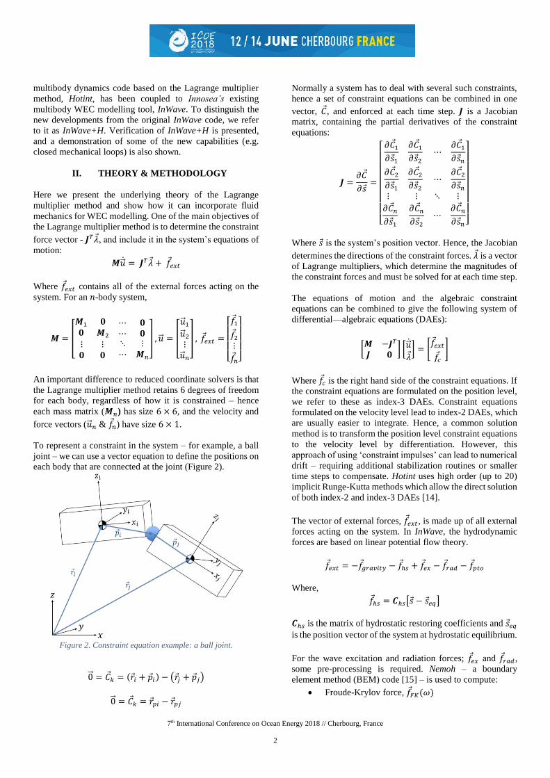
To represent a constraint in the system – for example, a ball

joint – we can use a vector equation to define the positions on

each body that are connected at the joint (Figure 2).

Figure 2. Constraint equation example: a ball joint.

0⃗⃗ = 𝐶𝑘 = (𝑟𝑖 + 𝑝𝑖) − (𝑟𝑗 + 𝑝𝑗)

0⃗⃗ = 𝐶𝑘 = 𝑟𝑝𝑖 − 𝑟𝑝𝑗

Normally a system has to deal with several such constraints,

hence a set of constraint equations can be combined in one

vector, 𝐶, and enforced at each time step. 𝑱 is a Jacobian

matrix, containing the partial derivatives of the constraint

equations:

𝑱 =𝜕𝐶

𝜕𝑠=

[ 𝜕𝐶1

𝜕𝑠1

𝜕𝐶1

𝜕𝑠2

𝜕𝐶2

𝜕𝑠1

𝜕𝐶2

𝜕𝑠2

⋯𝜕𝐶1

𝜕𝑠𝑛

⋯𝜕𝐶2

𝜕𝑠𝑛

⋮ ⋮

𝜕𝐶𝑛

𝜕𝑠1

𝜕𝐶𝑛

𝜕𝑠2

⋱ ⋮

⋯𝜕𝐶𝑛

𝜕𝑠𝑛 ]

Where 𝑠 is the system’s position vector. Hence, the Jacobian

determines the directions of the constraint forces. 𝜆 is a vector

of Lagrange multipliers, which determine the magnitudes of

the constraint forces and must be solved for at each time step.

The equations of motion and the algebraic constraint

equations can be combined to give the following system of

differential—algebraic equations (DAEs):

[𝑴 −𝑱𝑇

𝑱 𝟎] [�̇⃗⃗�

𝜆] = [

𝑓𝑒𝑥𝑡

𝑓𝑐]

Where 𝑓𝑐 is the right hand side of the constraint equations. If

the constraint equations are formulated on the position level,

we refer to these as index-3 DAEs. Constraint equations

formulated on the velocity level lead to index-2 DAEs, which

are usually easier to integrate. Hence, a common solution

method is to transform the position level constraint equations

to the velocity level by differentiation. However, this

approach of using ‘constraint impulses’ can lead to numerical

drift – requiring additional stabilization routines or smaller

time steps to compensate. Hotint uses high order (up to 20)

implicit Runge-Kutta methods which allow the direct solution

of both index-2 and index-3 DAEs [14].

The vector of external forces, 𝑓𝑒𝑥𝑡 , is made up of all external

forces acting on the system. In InWave, the hydrodynamic

forces are based on linear potential flow theory.

𝑓𝑒𝑥𝑡 = −𝑓𝑔𝑟𝑎𝑣𝑖𝑡𝑦 − 𝑓ℎ𝑠 + 𝑓𝑒𝑥 − 𝑓𝑟𝑎𝑑 − 𝑓𝑝𝑡𝑜

Where,

𝑓ℎ𝑠 = 𝑪ℎ𝑠[𝑠 − 𝑠𝑒𝑞]

𝑪ℎ𝑠 is the matrix of hydrostatic restoring coefficients and 𝑠𝑒𝑞

is the position vector of the system at hydrostatic equilibrium.

For the wave excitation and radiation forces; 𝑓𝑒𝑥 and 𝑓𝑟𝑎𝑑,

some pre-processing is required. Nemoh – a boundary

element method (BEM) code [15] – is used to compute:

Froude-Krylov force, 𝑓𝐹𝐾(𝜔)

7th International Conference on Ocean Energy 2018 // Cherbourg, France

3

Diffraction force, 𝑓𝑑𝑖𝑓𝑓(𝜔)

Added mass matrices, 𝑨(𝜔)

Radiation damping matrices, 𝑩(𝜔)

We refer to these frequency-domain hydrodynamic

coefficients collectively as the ‘hydrodynamic database’

(HDB). The wave excitation impulse response function

(IRF), 𝑲𝑒𝑥(𝜏) can then be obtained by combining 𝑓𝐹𝐾(𝜔) and

𝑓𝑑𝑖𝑓𝑓(𝜔) and computing the following integral:

𝑲𝑒𝑥(𝑡) =1

2𝜋∫ 𝑓𝑒𝑥

+∞

−∞

(𝜔)𝑒𝑖𝜔𝑡𝑑𝜔

𝑓𝑒𝑥(𝑡) can then be computed by convolving the excitation

impulse response with the wave elevation:

𝑓𝑒𝑥(𝑡) = ∫ 𝑲𝑒𝑥

+∞

−∞

(𝜏)𝜂(𝑡 − 𝜏)𝑑𝜏

Similarly, the radiation impulse response function (RIRF),

𝑲𝑟𝑎𝑑(𝑡) and 𝑓𝑟𝑎𝑑(𝑡) can be obtained by computing the

following integrals:

𝑲𝑟𝑎𝑑(𝑡) =2

𝜋∫ 𝑩

+∞

0

(𝜔) cos𝜔𝑡 𝑑𝜔

𝑓𝑟𝑎𝑑(𝑡) = ∫ 𝑲𝑟𝑎𝑑

𝑡

0

(𝑡 − 𝜏)�⃗⃗�(𝜏)𝑑𝜏

The radiation force requires that the system’s added mass at

infinite frequency, 𝑨∞, is added to the system’s mass matrix:

(𝑴 + 𝑨∞)�̇⃗⃗� = 𝑱𝑇𝜆 + 𝑓𝑒𝑥𝑡

The inclusion of 𝑨∞ can be difficult in some multibody

dynamics codes. For example, Chrono [16] uses integration

routines that do not assemble the entire system mass matrix,

which prohibits the addition of the full infinite added mass

matrix. Similarly, Simscape Multibody does not permit direct

modification of the full system mass matrix. However, Hotint

does permit access to the entire system’s mass matrix,

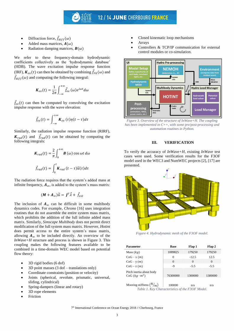
allowing 𝑨∞ to be included directly. An overview of the

InWave+H structure and process is shown in Figure 3. This

coupling makes the following features available to be

combined in a time-domain WEC model based on potential

flow theory:

3D rigid bodies (6 dof)

3D point masses (3 dof – translations only)

Coordinate constraints (position or velocity)

Joints (spherical, revolute, prismatic, universal,

sliding, cylindrical)

Spring-dampers (linear and rotary)

3D rope elements

Friction

Closed kinematic loop mechanisms

Arrays

Controllers & TCP/IP communication for external

control modules or co-simulation.

Figure 3. Overview of the structure of InWave+H. The coupling

has been implemented in C++, with some pre/post-processing and

automation routines in Python.

III. VERIFICATION

To verify the accuracy of InWave+H, existing InWave test

cases were used. Some verification results for the F3OF

model used in the WEC3 and NumWEC projects [2], [17] are

presented.

Figure 4. Hydrodynamic mesh of the F3OF model.

Parameter Base Flap 1 Flap 2

Mass (𝑘𝑔) 1089825 179250 179250

CoG – x (𝑚) 0 -12.5 12.5

CoG – y (𝑚) 0 0 0

CoG – z (𝑚) -9 -5.5 -5.5

Pitch inertia about body

CoG (𝑘𝑔 ∙ 𝑚2) 76300000 1300000 1300000

Mooring stiffness (𝑁 𝑚⁄ ) 100000 n/a n/a

Table 1. Key Characteristics of the F3OF Model.

7th International Conference on Ocean Energy 2018 // Cherbourg, France

4

A useful decay test to check the model’s hydrodynamic

interactions is to give one flap a 10° displacement in still

water, and let the radiated waves excite the other flap (Figure

5).

Figure 5. Decay test initial conditions: flap 1 given an initial offset

of 10 degrees.

Figure 6. Flap 1 pitch angle - decay test results.

Figure 7. Flap 2 pitch angle - decay test results.

Figures 6 and 7 show some small discrepancies between the

codes in both natural period and amplitude. This has been

attributed to different methods being used to compute the

HDB - future work will investigate these differences.

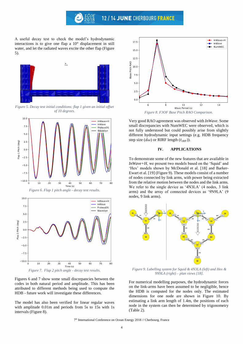
The model has also been verified for linear regular waves

with amplitude 0.01m and periods from 5s to 15s with 1s

intervals (Figure 8).

Figure 8. F3OF Base Pitch RAO Comparison.

Very good RAO agreement was observed with InWave. Some

small discrepancies with NumWEC were observed, which is

not fully understood but could possibly arise from slightly

different hydrodynamic input settings (e.g. HDB frequency

step size (𝑑𝜔) or RIRF length (𝑡𝐼𝑅𝐹)).

IV. APPLICATIONS

To demonstrate some of the new features that are available in

InWave+H, we present two models based on the ‘Squid’ and

‘Hex’ models shown by McDonald et al. [18] and Barker-

Ewart et al. [19] (Figure 9). These models consist of a number

of nodes connected by link arms, with power being extracted

from the relative motion between the nodes and the link arms.

We refer to the single device as ‘4N3LA’ (4 nodes, 3 link

arms) and the array of connected devices as ‘9N9LA’ (9

nodes, 9 link arms).

For numerical modelling purposes, the hydrodynamic forces

on the link-arms have been assumed to be negligible, hence

the HDB is computed for the nodes only. The estimated

dimensions for one node are shown in Figure 10. By

estimating a link arm length of 1.4m, the positions of each

node in the system can then be determined by trigonometry

(Table 2).

Figure 9. Labelling system for Squid & 4N3LA (left) and Hex &

9N9LA (right) – plan views [18].

7th International Conference on Ocean Energy 2018 // Cherbourg, France

5

Figure 10. Estimated node dimensions used in the 4N3LA and

9N9LA models.

Node CoG -x

(m)

CoG – y

(m)

CoG – z

(m)

S3 0 0 -0.3

C1 0.7 -1.21 -0.3

S1 0 -2.42 -0.3

S2 2.1 -1.21 -0.3

Table 2. 4N3LA - Node Positions used in the 4N3LA and 9N9LA

models.

Based on the estimates shown in Figure 10 and Table 2, the

hydrodynamic mesh was created (Figure 11) and the HDB

computed with Nemoh.

Figure 11. 4N3LA mesh.

The link arms are then included in the mechanical model, with

their centre of gravity at a depth of 0.4m. They are assumed

to be neutrally buoyant. Between each link arm and node,

there is a power take-off (PTO) absorbing power from the

relative pitch and yaw degrees of freedom. To model this, we

combined two constraint types: firstly, a Lagrange multiplier

constraint takes care of the spherical joint kinematics by using

a vector constraint equation to ensure that the designated

points on each body are exactly co-located, but can rotate

freely. Secondly, a penalty constraint applies angular stiffness

and damping torques to the relative pitch and yaw motion

between the bodies (Figure 12). The penalty constraint

permits different PTO stiffness and damping settings to be

used (𝐾𝑃𝑇𝑂 and 𝐶𝑃𝑇𝑂) in the model, and from the damping

torque we can estimate the power produced.

Figure 12. Schematic of the relative pitch & yaw PTOs applied

between each node and link arm.

3D rope elements were used to model the mooring system,

with rope connection points included as 3D mass elements

(Figure 13).

Figure 13. Overview of the time-domain model in Hotint GUI.

The stability of the system has been checked by observing the

system’s response in small amplitude regular waves (Figure

14).

Figure 14. Pitch angle of the 4N3LA rear node (S2) for regular

waves.

The model’s power output can be obtained by multiplying the

penalty constraint’s damping torque by the relevant angular

velocity (either relative pitch or relative yaw between node

and link arm). These individual PTO power outputs can be

7th International Conference on Ocean Energy 2018 // Cherbourg, France

6

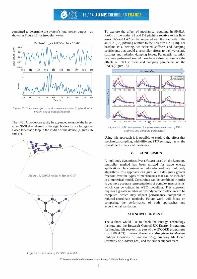
combined to determine the system’s total power output – as

shown in Figure 15 for irregular waves.

Figure 15. Time series for irregular wave elevation (top) and total

system power output (bottom).

The 4N3LA model can easily be expanded to model the larger

array, 9N9LA – where 6 of the rigid bodies form a hexagonal

closed kinematic loop in the middle of the device (Figures 16

and 17).

Figure 16. 9N9LA model in Hotint GUI.

Figure 17. Plan view of the 9N9LA model.

To explore the effect of mechanical coupling in 9N9LA,

RAOs of the nodes S2 and D1 pitching relative to the link-

arms LA5 and LA2 can be compared with the rear node of the

4N3LA (S2) pitching relative to the link arm LA2 [18]. For

baseline PTO setting, we selected stiffness and damping

coefficients that would give similar efforts to the hydrostatic

stiffness and radiation damping forces. Parametric variation

has been performed around these base values to compare the

effects of PTO stiffness and damping parameters on the

RAOs (Figure 18).

Figure 18. RAO comparison for parametric variation of PTO

stiffness and damping parameters.

Using this approach it is possible to explore the effect that

mechanical coupling, with different PTO settings, has on the

overall performance of the device.

V. CONCLUSION

A multibody dynamics solver (Hotint) based on the Lagrange

multiplier method has been utilized for wave energy

applications. In constrast to reduced-coordinate multibody

algorithms, this approach can give WEC designers greater

freedom over the types of mechanisms that can be included

in a numerical model. Constraints can be combined in order

to get more accurate representations of complex mechanisms,

which can be critical in WEC modelling. This approach

requires a greater number of hydrodynamic coefficients to be

computed, which may impact performance compared to

reduced-coordinate methods. Future work will focus on

comparing the performance of both approaches and

experimental validation.

ACKNOWLEDGMENT

The authors would like to thank the Energy Technology

Institute and the Research Council UK Energy Programme

for funding this research as part of the IDCORE programme

(EP/J500847/1). Sincere thanks are also given to Maxime

Philippe (formerly of Innosea SAS), Anthony McDonald

(formerly of Albatern Ltd.) and the Hotint support team.

7th International Conference on Ocean Energy 2018 // Cherbourg, France

7

REFERENCES

[1] EMEC, “Wave developers,” 2017. [Online].

Available: http://www.emec.org.uk/marine-

energy/wave-developers/.

[2] A. Combourieu, M. Lawson, A. Babarit, K. Ruehl,

A. Roy, R. Costello, P. L. Weywada, and H. Bailey,

“WEC3 : Wave Energy Converter Code Comparison

Project,” in Proceedings of the 11th European Wave

and Tidal Conference EWTEC 2015, 2015.

[3] F. Wendt, Y. Yu, K. Nielsen, K. Ruehl, T. Bunnik, I.

Touzon, B. W. Nam, J. S. Kim, K. Kim, C. E.

Janson, K. Jakobsen, S. Crowley, L. Vega, K.

Rajagopalan, T. Mathai, D. Greaves, E. Ransley, P.

Lamont-kane, W. Sheng, R. Costello, B. Kennedy,

S. Thomas, P. Heras, H. Bingham, A. Kurniawan,

M. M. Kramer, D. Ogden, S. Girardin, P.

Wuillaume, D. Steinke, S. Beatty, P. Schofield, J.

Jansson, and J. Hoffman, “International Energy

Agency Ocean Energy Systems Task 10 Wave

Energy Converter Modeling Verification and

Validation,” in Proceedings of the 12th European

Wave and Tidal Conference, EWTEC 2017, 2017,

pp. 1197--1–10.

[4] J. Cruz, E. Mackay, M. Livingstone, and B. Child,

“Validation of Design and Planning Tools for Wave

Energy Converters (WECs),” in 1st Marine Energy

Technology Symposium METS13, 2013.

[5] M. Lawson, Y. Yu, K. Ruehl, and C. Michelen,

“Improving and Validating the WEC-Sim Wave

Energy Converter Modeling Code,” Proc. 3rd Mar.

Energy Technol. Symp. METS2015, no. April, 2015.

[6] A. Combourieu, M. Philippe, F. Rongère, and A.

Babarit, “InWave : A New Flexible Design Tool

Dedicated to Wave Energy Converters,” in ASME

2014 33rd International Conference on Ocean,

Offshore and Arctic Engineering, OMAE2014, 2014.

[7] J. Lucas, M. Livingstone, M. Vuorinen, and J. Cruz,

“Development of a wave energy converter (WEC)

design tool - application to the WaveRoller WEC

including validation of numerical estimates,” in

Proceedings of the 4th International Conference on

Ocean Energy, ICOE 2012, 2012.

[8] R. S. Nicoll, C. F. Wood, and A. R. Roy,

“Comparison of Physical Model Tests With a Time

Domain Simulation Model of a Wave Energy

Converter,” in Proceedings of the ASME 2012 31st

International Conference on Ocean, Offshore and

Arctic Engineering, 2012.

[9] M. Ó’Catháin, B. J. Leira, J. V. Ringwood, and J. C.

Gilloteaux, “A modelling methodology for multi-

body systems with application to wave-energy

devices,” Ocean Eng., vol. 35, no. 13, pp. 1381–

1387, 2008.

[10] F. Rongère and A. H. Clément, “Systematic

dynamic modeling and simulation of multibody

offshore structures: Application to wave energy

converters,” in ASME 2013 32nd International

Conference on Ocean, Offshore and Arctic

Engineering, 2013.

[11] D. Baraff, “Linear-Time Dynamics using Lagrange

Multipliers,” in Computer Graphics Proceedings,

Annual Conference Series (SIGGRAPH 96), 1996,

pp. 137–146.

[12] F. Paparella, “Modeling and Control of a Multibody

Hinge-Barge Wave Energy Converter,” Maynooth

University, 2017.

[13] W. Edwards, D. Findlay, D. Scott, and P. Graham,

“SHAPE Pilot Albatern: Numerical Simulation of

Extremely Large Interconnected Wavenet Arrays,”

2014.

[14] J. Gerstmayr, “Hotint – A C++ Environment for the

Simulation of Multibody Dynamics Systems and

Finite Elements,” in Multibody Dynamics 2009,

ECCOMAS Thematic Conference, 2009, no. July,

pp. 1–20.

[15] A. Babarit and G. Delhommeau, “Theoretical and

numerical aspects of the open source BEM solver

NEMOH,” in Proceedings of the 11th European

Wave and Tidal Energy Conference., 2015, pp. 1–

12.

[16] H. Mazhar, T. Heyn, A. Pazouki, D. Melanz, A.

Seidl, A. Bartholomew, A. Tasora, and D. Negrut,

“Chrono: a parallel multi-physics library for rigid-

body, flexible-body, and fluid dynamics,” Mech. Sci,

vol. 4, no. 1, pp. 49–64, 2013.

[17] A. Babarit, J. Hals, A. Kurniawan, M. Muliawan, T.

Moan, and J. Krokstad, “The NumWEC project,”

2011.

[18] A. McDonald, Q. Xiao, D. Forehand, and D.

Findlay, “Experimental Investigation of Array

Effects for a Mechanically Coupled WEC Array,” in

Proceedings of the Twelfth European Wave and

Tidal Energy Conference, 2017, pp. 929–1--9.

[19] L. Barker-Ewart, P. R. Thies, T. Stratford, and N.

Barltrop, “Optimising structural loading and power

production for floating wave energy converters,” in

Proceedings of the Twelfth European Wave and

Tidal Energy Conference, 2017, pp. 840–1--10.

View publication statsView publication stats