TASK 1

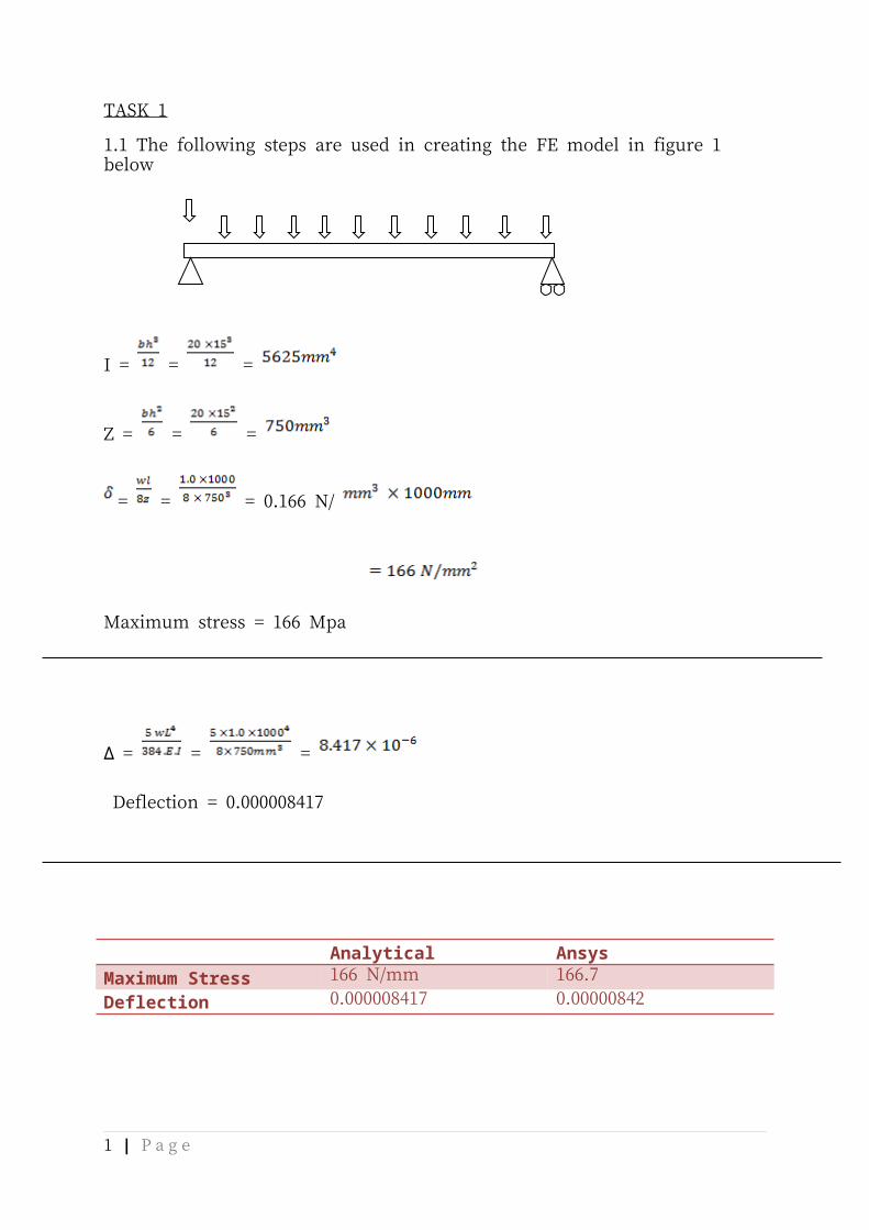
1.1 The following steps are used in creating the FE model in figure 1 below

I = = =

Z = = =

= = = 0.166 N/

Maximum stress = 166 Mpa

Δ = = =

Deflection = 0.000008417

Analytical AnsysMaximum Stress 166 N/mm 166.7Deflection 0.000008417 0.00000842

1 | P a g e

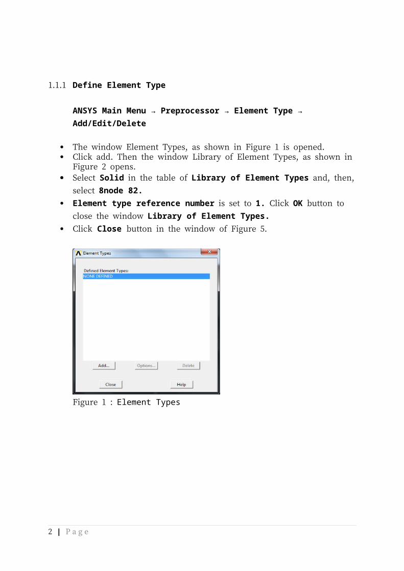
1.1.1 Define Element Type

ANSYS Main Menu → Preprocessor → Element Type → Add/Edit/Delete

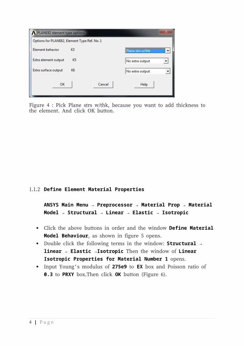
The window Element Types, as shown in Figure 1 is opened. Click add. Then the window Library of Element Types, as shown in Figure 2 opens. Select Solid in the table of Library of Element Types and, then, select 8node 82. Element type reference number is set to 1. Click OK button to close the window

Library of Element Types. Click Close button in the window of Figure 5.

Figure 1 : Element Types

Figure 2 : Library of Element Types

2 | P a g e

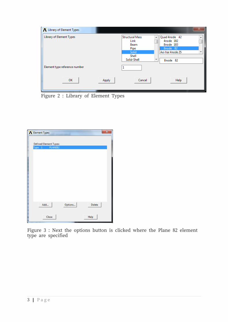
Figure 3 : Next the options button is clicked where the Plane 82 element type are specified

Figure 4 : Pick Plane strs w/thk, because you want to add thickness to the element. And click OK button.

3 | P a g e

1.1.2 Define Element Material Properties

ANSYS Main Menu → Preprocessor → Material Prop → Material Model → Structural → Linear → Elastic → Isotropic

Click the above buttons in order and the window Define Material Model Behaviour, as shown in figure 5 opens.

Double click the following terms in the window: Structural → linear → Elastic →Isotropic Then the window of Linear Isotropic Properties for Material Number 1 opens.

Input Young’s modulus of 275e9 to EX box and Poisson ratio of 0.3 to PRXY box.Then click OK button (Figure 6).

Figure 5 : Windows of Linear Isotropic Property for material Number 1

4 | P a g e

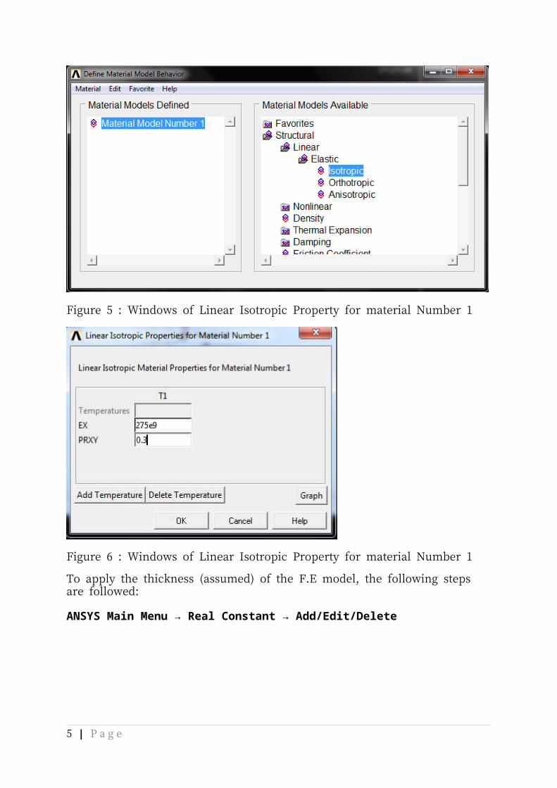
Figure 6 : Windows of Linear Isotropic Property for material Number 1

To apply the thickness (assumed) of the F.E model, the following steps are followed:

ANSYS Main Menu → Real Constant → Add/Edit/Delete

Figure 7 above, Shows the Real Constants Sets Window before any of the constants have been defined and the Element type for Real Constants Window which pops up when you click Add in the Defined Real Constants Sets Window.

5 | P a g e

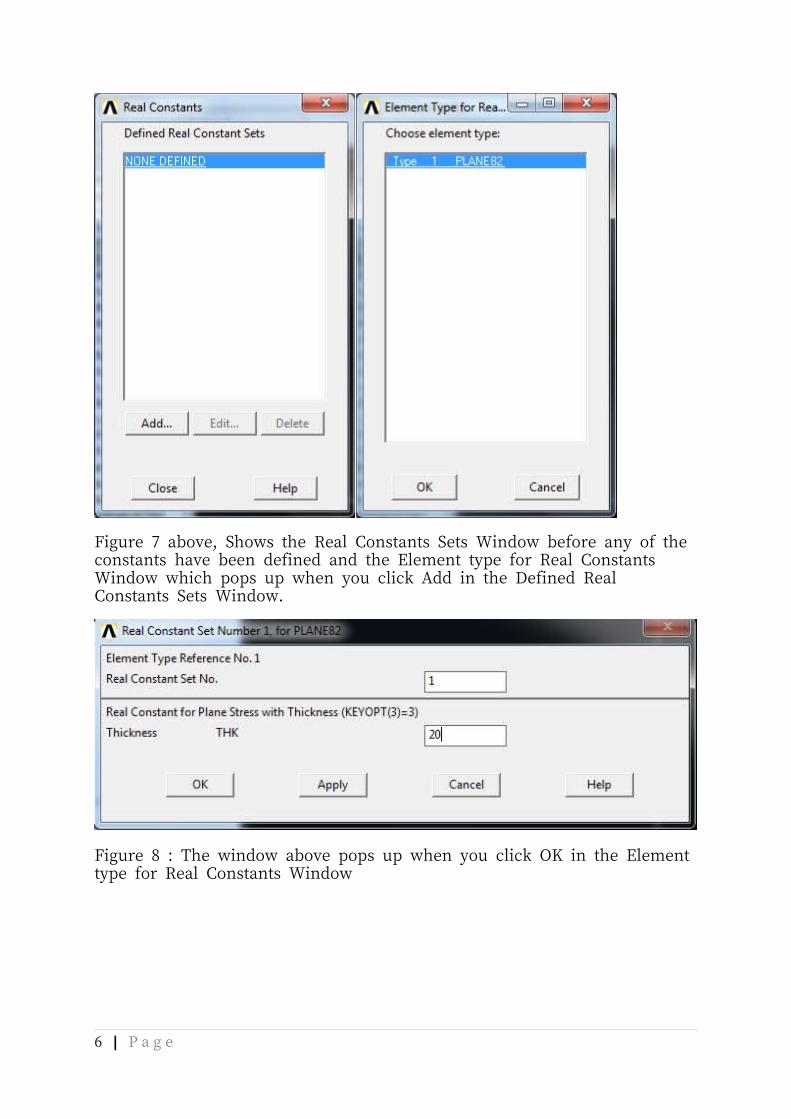
Figure 8 : The window above pops up when you click OK in the Element type for Real Constants Window

Figure 9 : Number of sets of real constants

6 | P a g e

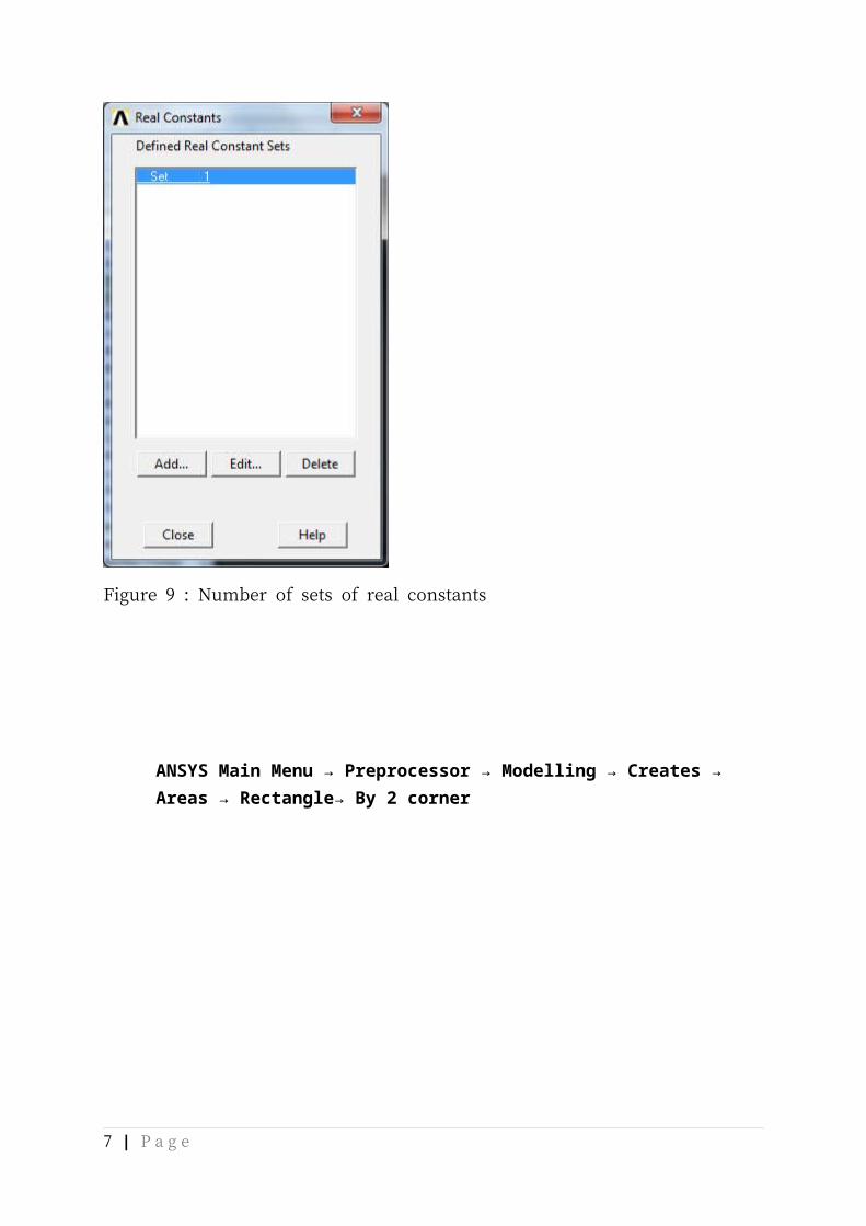
ANSYS Main Menu → Preprocessor → Modelling → Creates → Areas → Rectangle→ By 2 corner

Figure 10 : The following window will come up, input the figures as seen in the picture above

Figure 11 : Click apply and the above window will appear

7 | P a g e

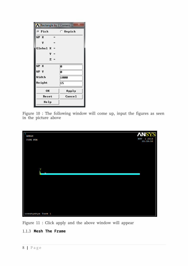
1.1.3 Mesh The Frame

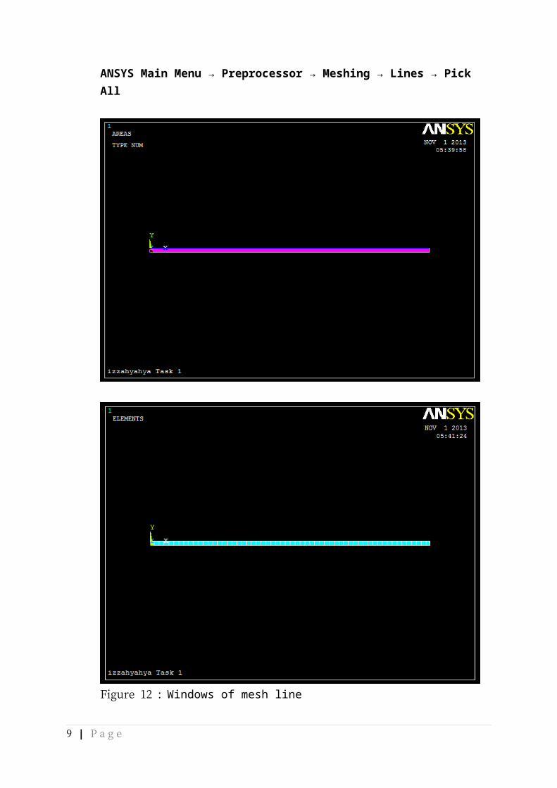
ANSYS Main Menu → Preprocessor → Meshing → Lines → Pick All

Figure 12 : Windows of mesh line

8 | P a g e

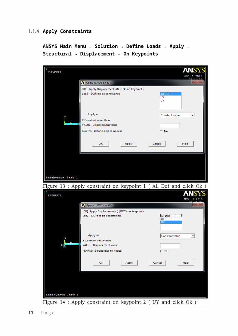
1.1.4 Apply Constraints

ANSYS Main Menu → Solution → Define Loads → Apply → Structural → Displacement → On Keypoints

Figure 13 : Apply constraint on keypoint 1 ( All Dof and click Ok )

Figure 14 : Apply constraint on keypoint 2 ( UY and click Ok )

9 | P a g e

1.1.5 Apply Loads ANSYS Main Menu → Solution → Define Loads → Apply → Structural → Pressure →On Line

Figure 15 : Apply the pressure on Lines ( click Pick All )

Figure 16 : Enter the 0.05 for the load PRES value

10 | P a g e

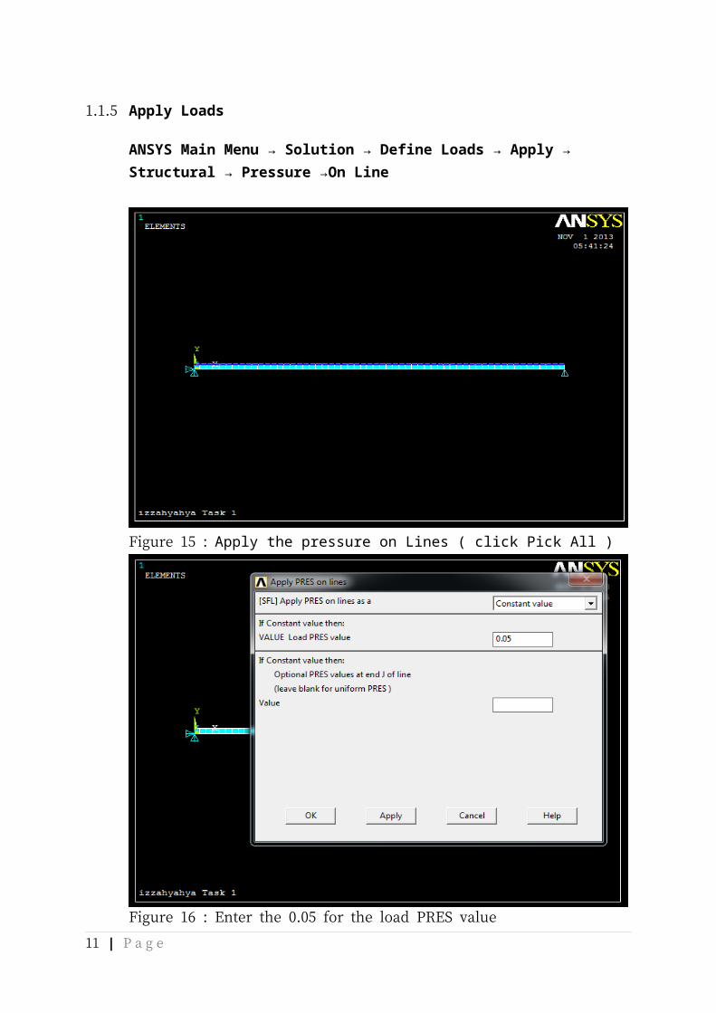
Figure 17 : The applied loads and constraints now appear

1.1.6 Solve The System

ANSYS Main Menu → Solution → Solve → Current LS

11 | P a g e

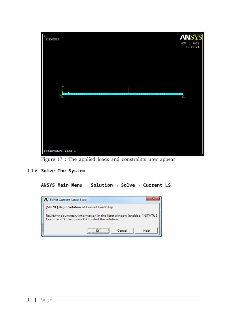
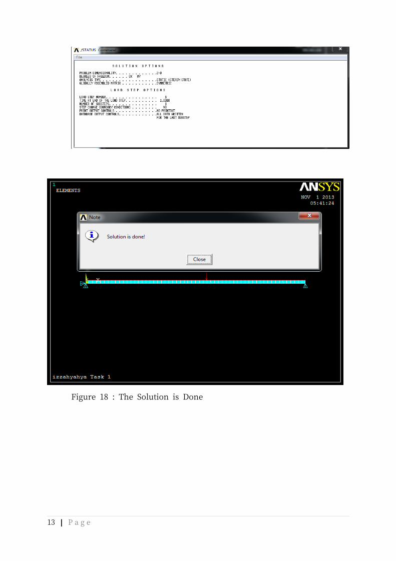
Figure 18 : The Solution is Done

12 | P a g e

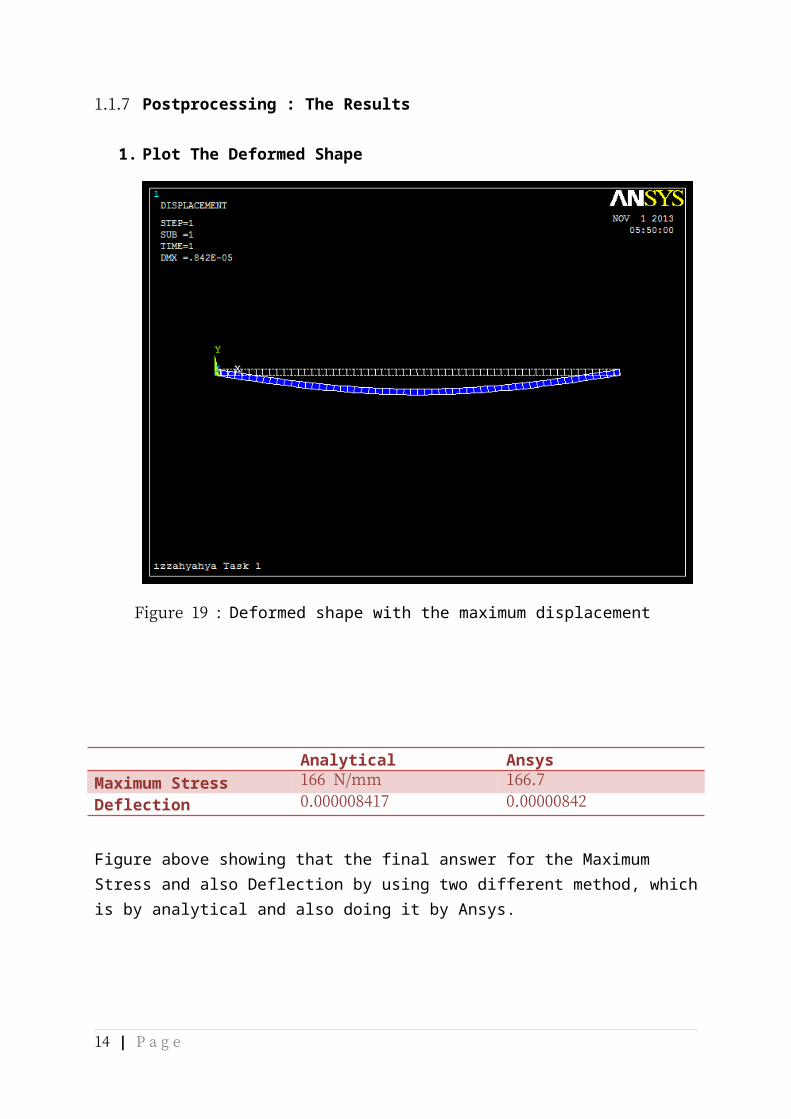
1.1.7 Postprocessing : The Results

1. Plot The Deformed Shape

Figure 19 : Deformed shape with the maximum displacement

Analytical AnsysMaximum Stress 166 N/mm 166.7Deflection 0.000008417 0.00000842

Figure above showing that the final answer for the Maximum Stress and also Deflection by using two different method, which is by analytical and also doing it by Ansys.

13 | P a g e

2. Plot Principal Stress Distribution

Figure 20 : Stress Distribution 1

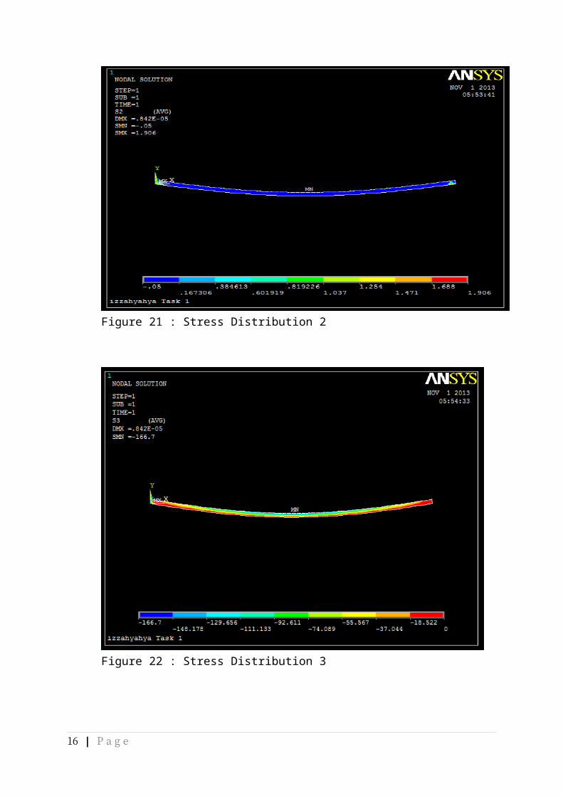
Figure 21 : Stress Distribution 2

14 | P a g e

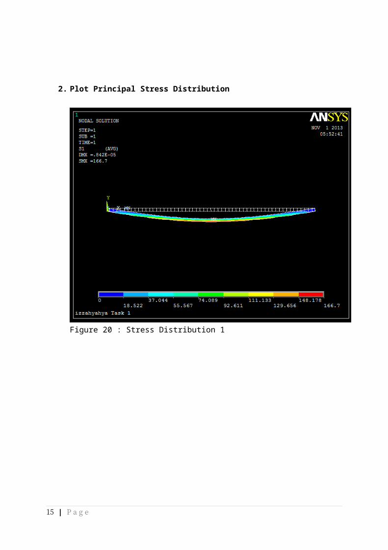
Figure 22 : Stress Distribution 3

15 | P a g e

3. Value and position of the maximum and minimum stress

Figure 23 : shows the von misses stress plot for the beam

The color bar shows the displacement at the different nodal points. The colors help indicate where failure will occur first (the red side), and blue is where there is minimal stress hence minimal displacement. The value of stress decreases as the colors change as you go from right to left as the colors change from red to blue.

Maximum : 166.7

Minimum : 2.005

16 | P a g e

17 | P a g e