Near-Lossless Compression for Large Traffic Networksjaillet/general/NLComp_A1.pdf · the country...
10
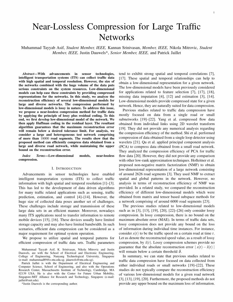
1 Near-Lossless Compression for Large Traffic Networks Muhammad Tayyab Asif, Student Member, IEEE, Kannan Srinivasan, Member, IEEE, Nikola Mitrovic, Student Member, IEEE, Justin Dauwels*, Senior Member, IEEE, and Patrick Jaillet Abstract—With advancements in sensor technologies, intelligent transportation systems (ITS) can collect traffic data with high spatial and temporal resolution. However, the size of the networks combined with the huge volume of the data puts serious constraints on the system resources. Low-dimensional models can help ease these constraints by providing compressed representations for the networks. In this study, we analyze the reconstruction efficiency of several low-dimensional models for large and diverse networks. The compression performed by low-dimensional models is lossy in nature. To address this issue, we propose a near-lossless compression method for traffic data by applying the principle of lossy plus residual coding. To this end, we first develop low-dimensional model of the network. We then apply Huffman coding in the residual layer. The resultant algorithm guarantees that the maximum reconstruction error will remain below a desired tolerance limit. For analysis, we consider a large and heterogeneous test network comprising of more than 18000 road segments. The results show that the proposed method can efficiently compress data obtained from a large and diverse road network, while maintaining the upper bound on the reconstruction error. Index Terms—Low-dimensional models, near-lossless compression. I. I NTRODUCTION Advancements in sensor technologies have enabled intelligent transportation systems (ITS) to collect traffic information with high spatial and temporal resolution [1]–[3]. This has led to the development of data driven algorithms for many traffic related applications such as sensing, traffic prediction, estimation, and control [4]–[14]. However, the huge size of collected data poses another set of challenges. These challenges include storage and transmission of these large data sets in an efficient manner. Moreover, nowadays many ITS applications need to transfer information to remote mobile devices [15], [16]. These devices usually have limited storage capacity and may also have limited bandwidth. In such scenarios, efficient data compression can be considered as a major requirement for optimal system operation. We propose to utilize spatial and temporal patterns for efficient compression of traffic data sets. Traffic parameters Muhammad Tayyab Asif, K. Srinivasan, Nikola Mitrovic and Justin Dauwels, are with the School of Electrical and Electronic Engineering, College of Engineering, Nanyang Technological University, Singapore (e-mail: [email protected]; [email protected]). Patrick Jaillet is with the Department of Electrical Engineering and Computer Science, School of Engineering, and also with the Operations Research Center, Massachusetts Institute of Technology, Cambridge, MA 02139 USA. He is also with the Center for Future Urban Mobility, Singapore-MIT Alliance for Research and Technology, Singapore (e-mail: [email protected]). *Justin Dauwels is the corresponding author. tend to exhibit strong spatial and temporal correlations [7], [17]. These spatial and temporal relationships can help to obtain a low-dimensional representation for a given network. The low-dimensional models have been previously considered for applications related to feature selection [7], [17], [18], missing data imputation [4], [12] and estimation [3], [14]. Low-dimensional models provide compressed state for a given network. Hence, they are naturally suited for data compression. Previous studies related to traffic data compression have mostly focused on data from a single road or small subnetworks [19]–[22]. Yang et al. compressed flow data obtained from individual links using 2D wavelet transform [19]. They did not provide any numerical analysis regarding the compression efficiency of the method. Shi et al. performed compression of data obtained from a single loop detector using wavelets [21]. Qu et al. applied principal component analysis (PCA) to compress data obtained from a small road network. They analyzed the compression efficiency of PCA for traffic flow data [20]. However, they did not provide any comparison with other low-rank approximation techniques. Hofleitner et al. proposed non-negative matrix factorization (NMF) to obtain low-dimensional representation of a large network consisting of around 2626 road segments [3]. They used NMF to extract spatial and global patterns in the network. However, no analysis in terms of reconstruction efficiency of NMF was provided. In a related study, we compared the reconstruction efficiency of different low-dimensional models which were obtained from matrix and tensor based subspace methods for a network comprising of around 6000 road segments [23]. The previous studies related to low-dimensional models such as in [3], [13], [19], [20], [22]–[26] only consider lossy compression. In lossy compression, there is no bound on the maximum absolute error (MAE). In terms of traffic data sets, lossy compression does not provide any bound on the loss of information during individual time instances. For instance, consider x(t ) to be the traffic speed on a certain road at time t . Let us denote the reconstructed speed value, as a result of lossy compression, by ˆ x(t ). Lossy compression schemes provide no guarantee that the absolute reconstruction error | x(t ) − ˆ x(t ) | will remain below a certain threshold δ . In summary, we can state that previous studies related to traffic data compression have focused on data collected from either individual roads or small networks [19]–[22]. These studies do not typically compare the reconstruction efficiency of various low-dimensional models for a given road network [3], [13], [19], [20]. Furthermore, the proposed methods do not provide any upper bound on the maximum loss of information.
Transcript of Near-Lossless Compression for Large Traffic Networksjaillet/general/NLComp_A1.pdf · the country...
1
Near-Lossless Compression for Large Traffic
NetworksMuhammad Tayyab Asif, Student Member, IEEE, Kannan Srinivasan, Member, IEEE, Nikola Mitrovic, Student
Member, IEEE, Justin Dauwels*, Senior Member, IEEE, and Patrick Jaillet
Abstract—With advancements in sensor technologies,intelligent transportation systems (ITS) can collect traffic datawith high spatial and temporal resolution. However, the size ofthe networks combined with the huge volume of the data putsserious constraints on the system resources. Low-dimensionalmodels can help ease these constraints by providing compressedrepresentations for the networks. In this study, we analyze thereconstruction efficiency of several low-dimensional models forlarge and diverse networks. The compression performed bylow-dimensional models is lossy in nature. To address this issue,we propose a near-lossless compression method for traffic databy applying the principle of lossy plus residual coding. To thisend, we first develop low-dimensional model of the network. Wethen apply Huffman coding in the residual layer. The resultantalgorithm guarantees that the maximum reconstruction errorwill remain below a desired tolerance limit. For analysis, weconsider a large and heterogeneous test network comprisingof more than 18000 road segments. The results show that theproposed method can efficiently compress data obtained from alarge and diverse road network, while maintaining the upperbound on the reconstruction error.
Index Terms—Low-dimensional models, near-losslesscompression.
I. INTRODUCTION
Advancements in sensor technologies have enabled
intelligent transportation systems (ITS) to collect traffic
information with high spatial and temporal resolution [1]–[3].
This has led to the development of data driven algorithms
for many traffic related applications such as sensing, traffic
prediction, estimation, and control [4]–[14]. However, the
huge size of collected data poses another set of challenges.
These challenges include storage and transmission of these
large data sets in an efficient manner. Moreover, nowadays
many ITS applications need to transfer information to remote
mobile devices [15], [16]. These devices usually have limited
storage capacity and may also have limited bandwidth. In such
scenarios, efficient data compression can be considered as a
major requirement for optimal system operation.
We propose to utilize spatial and temporal patterns for
efficient compression of traffic data sets. Traffic parameters
Muhammad Tayyab Asif, K. Srinivasan, Nikola Mitrovic and JustinDauwels, are with the School of Electrical and Electronic Engineering,College of Engineering, Nanyang Technological University, Singapore(e-mail: [email protected]; [email protected]).
Patrick Jaillet is with the Department of Electrical Engineering andComputer Science, School of Engineering, and also with the OperationsResearch Center, Massachusetts Institute of Technology, Cambridge, MA02139 USA. He is also with the Center for Future Urban Mobility,Singapore-MIT Alliance for Research and Technology, Singapore (e-mail:[email protected]).
*Justin Dauwels is the corresponding author.
tend to exhibit strong spatial and temporal correlations [7],
[17]. These spatial and temporal relationships can help to
obtain a low-dimensional representation for a given network.
The low-dimensional models have been previously considered
for applications related to feature selection [7], [17], [18],
missing data imputation [4], [12] and estimation [3], [14].
Low-dimensional models provide compressed state for a given
network. Hence, they are naturally suited for data compression.
Previous studies related to traffic data compression have
mostly focused on data from a single road or small
subnetworks [19]–[22]. Yang et al. compressed flow data
obtained from individual links using 2D wavelet transform
[19]. They did not provide any numerical analysis regarding
the compression efficiency of the method. Shi et al. performed
compression of data obtained from a single loop detector using
wavelets [21]. Qu et al. applied principal component analysis
(PCA) to compress data obtained from a small road network.
They analyzed the compression efficiency of PCA for traffic
flow data [20]. However, they did not provide any comparison
with other low-rank approximation techniques. Hofleitner et al.
proposed non-negative matrix factorization (NMF) to obtain
low-dimensional representation of a large network consisting
of around 2626 road segments [3]. They used NMF to extract
spatial and global patterns in the network. However, no
analysis in terms of reconstruction efficiency of NMF was
provided. In a related study, we compared the reconstruction
efficiency of different low-dimensional models which were
obtained from matrix and tensor based subspace methods for
a network comprising of around 6000 road segments [23].
The previous studies related to low-dimensional models
such as in [3], [13], [19], [20], [22]–[26] only consider lossy
compression. In lossy compression, there is no bound on the
maximum absolute error (MAE). In terms of traffic data sets,
lossy compression does not provide any bound on the loss
of information during individual time instances. For instance,
consider x(t) to be the traffic speed on a certain road at time t.
Let us denote the reconstructed speed value, as a result of lossy
compression, by x(t). Lossy compression schemes provide no
guarantee that the absolute reconstruction error | x(t)− x(t) |will remain below a certain threshold δ .
In summary, we can state that previous studies related to
traffic data compression have focused on data collected from
either individual roads or small networks [19]–[22]. These
studies do not typically compare the reconstruction efficiency
of various low-dimensional models for a given road network
[3], [13], [19], [20]. Furthermore, the proposed methods do not
provide any upper bound on the maximum loss of information.
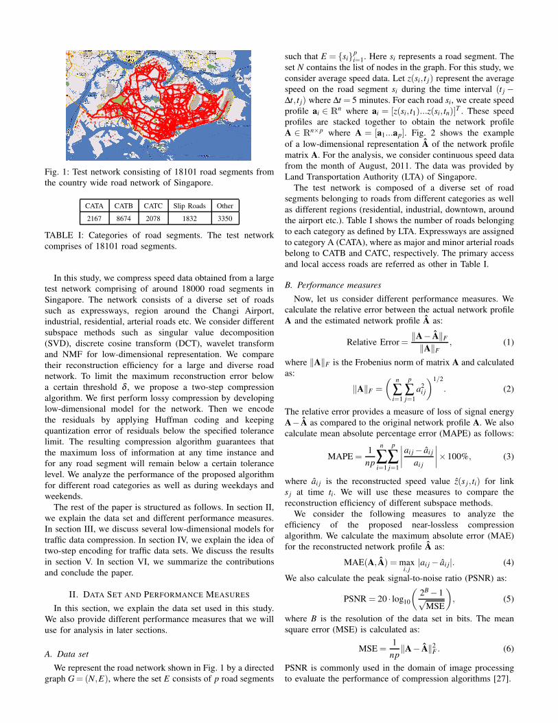
Fig. 1: Test network consisting of 18101 road segments from
the country wide road network of Singapore.
CATA CATB CATC Slip Roads Other
2167 8674 2078 1832 3350
TABLE I: Categories of road segments. The test network
comprises of 18101 road segments.
In this study, we compress speed data obtained from a large
test network comprising of around 18000 road segments in
Singapore. The network consists of a diverse set of roads
such as expressways, region around the Changi Airport,
industrial, residential, arterial roads etc. We consider different
subspace methods such as singular value decomposition
(SVD), discrete cosine transform (DCT), wavelet transform
and NMF for low-dimensional representation. We compare
their reconstruction efficiency for a large and diverse road
network. To limit the maximum reconstruction error below
a certain threshold δ , we propose a two-step compression
algorithm. We first perform lossy compression by developing
low-dimensional model for the network. Then we encode
the residuals by applying Huffman coding and keeping
quantization error of residuals below the specified tolerance
limit. The resulting compression algorithm guarantees that
the maximum loss of information at any time instance and
for any road segment will remain below a certain tolerance
level. We analyze the performance of the proposed algorithm
for different road categories as well as during weekdays and
weekends.
The rest of the paper is structured as follows. In section II,
we explain the data set and different performance measures.
In section III, we discuss several low-dimensional models for
traffic data compression. In section IV, we explain the idea of
two-step encoding for traffic data sets. We discuss the results
in section V. In section VI, we summarize the contributions
and conclude the paper.
II. DATA SET AND PERFORMANCE MEASURES
In this section, we explain the data set used in this study.
We also provide different performance measures that we will
use for analysis in later sections.
A. Data set
We represent the road network shown in Fig. 1 by a directed
graph G= (N,E), where the set E consists of p road segments
such that E = sipi=1. Here si represents a road segment. The
set N contains the list of nodes in the graph. For this study, we
consider average speed data. Let z(si, t j) represent the average
speed on the road segment si during the time interval (t j −∆t, t j) where ∆t = 5 minutes. For each road si, we create speed
profile ai ∈ Rn where ai = [z(si, t1)...z(si, tn)]T . These speed
profiles are stacked together to obtain the network profile
A ∈ Rn×p where A = [a1...ap]. Fig. 2 shows the example
of a low-dimensional representation A of the network profile
matrix A. For the analysis, we consider continuous speed data
from the month of August, 2011. The data was provided by
Land Transportation Authority (LTA) of Singapore.
The test network is composed of a diverse set of road
segments belonging to roads from different categories as well
as different regions (residential, industrial, downtown, around
the airport etc.). Table I shows the number of roads belonging
to each category as defined by LTA. Expressways are assigned
to category A (CATA), where as major and minor arterial roads
belong to CATB and CATC, respectively. The primary access
and local access roads are referred as other in Table I.
B. Performance measures
Now, let us consider different performance measures. We
calculate the relative error between the actual network profile
A and the estimated network profile A as:
Relative Error =‖A− A‖F
‖A‖F
, (1)
where ‖A‖F is the Frobenius norm of matrix A and calculated
as:
‖A‖F =
(
n
∑i=1
p
∑j=1
a2i j
)1/2
. (2)
The relative error provides a measure of loss of signal energy
A− A as compared to the original network profile A. We also
calculate mean absolute percentage error (MAPE) as follows:
MAPE =1
np
n
∑i=1
p
∑j=1
∣
∣
∣
∣
ai j − ai j
ai j
∣
∣
∣
∣
× 100%, (3)
where ai j is the reconstructed speed value z(s j , ti) for link
s j at time ti. We will use these measures to compare the
reconstruction efficiency of different subspace methods.
We consider the following measures to analyze the
efficiency of the proposed near-lossless compression
algorithm. We calculate the maximum absolute error (MAE)
for the reconstructed network profile A as:
MAE(A, A) = maxi, j
|ai j − ai j|. (4)
We also calculate the peak signal-to-noise ratio (PSNR) as:
PSNR = 20 · log10
(
2B − 1√MSE
)
, (5)
where B is the resolution of the data set in bits. The mean
square error (MSE) is calculated as:
MSE =1
np‖A− A‖2
F . (6)
PSNR is commonly used in the domain of image processing
to evaluate the performance of compression algorithms [27].
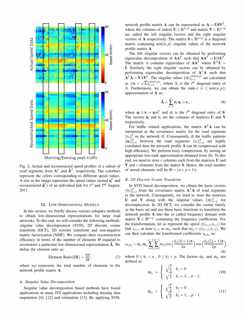
Fig. 2: Actual and reconstructed speed profiles of a subset of
road segments from AT and AT , respectively. The colorbars
represent the colors corresponding to different speed values.
A row in the image represents the speed values (actual aTi and
reconstructed aTi ) of an individual link for 1st and 2nd August,
2011.
III. LOW-DIMENSIONAL MODELS
In this section, we briefly discuss various subspace methods
to obtain low-dimensional representations for large road
networks. To this end, we will consider the following methods:
singular value decomposition (SVD), 2D discrete cosine
transform (DCT), 2D wavelet transform and non-negative
matrix factorization (NMF). We compare their reconstruction
efficiency in terms of the number of elements Θ required to
reconstruct a particular low-dimensional representation A. We
define the element ratio as:
Element Ratio(ER) =np
Θ, (7)
where np represents the total number of elements in the
network profile matrix A.
A. Singular Value Decomposition
Singular value decomposition based methods have found
applications in many ITS applications including missing data
imputation [4], [12] and estimation [13]. By applying SVD,
network profile matrix A can be represented as A = USVT ,
where the columns of matrix U ∈Rn×n and matrix V ∈Rp×p
are called the left singular vectors and the right singular
vectors of A respectively. The matrix S ∈Rn×p is a diagonal
matrix containing min(n, p) singular values of the network
profile matrix A.
The left singular vectors can be obtained by performing
eigenvalue decomposition of AAT such that AAT = UΛUT .
The matrix Λ contains eigenvalues of AAT where UT U =I. Similarly the right singular vectors can be obtained by
performing eigenvalue decomposition of AT A such that
AT A = VΛVT . The singular values σimin(n,p)i=1 are calculated
as σi =√
λimin(n,p)i=1 , where λi is the ith diagonal entry of
Λ. Furthermore, we can obtain the rank-r (r ≤ min(n, p))approximation of A as:
A =r
∑i=1
σi ui ⊗ vi, (8)
where ui ⊗ vi = uivTi and σi is the ith diagonal entry of S.
The vectors ui and vi are the columns of matrices U and V
respectively.
For traffic related applications, the matrix AT A can be
interpreted as the covariance matrix for the road segments
sipi in the network G. Consequently, if the traffic patterns
aipi=1 between the road segments sip
i=1 are highly
correlated then the network profile A can be compressed with
high efficiency. We perform lossy compression, by storing an
appropriate low-rank approximation obtained from (8). To this
end, we need to store r columns each from the matrices U and
V and r elements from the matrix S. Hence, the total number
of stored elements will be Θ = (n+ p+ 1)r.
B. 2D Discrete Cosine Transform
In SVD based decomposition, we obtain the basis vectors
vipi=1 from the covariance matrix AT A of road segments
in the network. Consequently, we need to store the matrices
U and V along with the singular values σiri=1 for
decompression. In 2D DCT, we consider the cosine family
as the basis set and use these basis functions to transform the
network profile A into the so called frequency domain with
matrix Y ∈ Rn×p containing the frequency coefficients. For
the transformation, let us represent the speed z(s j+1, ti+1) for
link s j+1 at time ti+1 as mi j such that mi j = z(s j+1, ti+1). We
can then calculate the transformed coefficients yk1k2as:
yk1k2=αk1
αk2
n−1
∑i=0
p−1
∑j=0
mi j cos(k1(2i+ 1)π
2n
)
cos(k2(2 j+ 1)π
2p
)
,
(9)
where 0 ≤ k1 < n , 0 ≤ k2 < p. The factors αk1and αk2
are
defined as:
αk1=
√
1n
k1 = 0√
2n
k1 = 1, ...n− 1,(10)
αk2=
√
1p
k2 = 0√
2p
k2 = 1, ...p− 1.(11)
As the basis functions are orthonormal, the inverse transform
can be easily calculated as:
mi j =n−1
∑k1=0
p−1
∑k2=0
αk1αk2
yk1k2cos
(k1(2i+ 1)π
2n
)
cos(k2(2 j+ 1)π
2p
)
,
(12)
where mi j is the estimated speed value z(s j+1, ti+1) for link
s j+1 at time ti+1. Traffic parameters such as speed and flow
tend to be highly correlated across the network [12], [28].
Therefore, we expect that most of the information contained
in the network profile A can be represented by considering a
small number of frequency components Θ and we can discard
the rest of the frequency components yk1k2= 0k1k2 6∈Ω. Here
Ω is the set of the indices of the frequency components used
for reconstruction of traffic data [23]. As the basis functions
are pre-specified, we only need to store the elements belonging
to the set Ω to reconstruct the network profile A.
C. Wavelets
Wavelet transforms have been widely used in compression
related applications including images [29], [30] and medical
data sets such as electroencephalogram (EEG) [31], [32].
Similar to DCT, wavelets also perform compression using a
pre-specified basis set. Wavelet based methods have also been
applied for compression of traffic related data sets [19], [21],
[22], [25]. However, these studies only analyze data obtained
from either individual links or small networks [19], [22].
Moreover, these studies have not compared the performance of
wavelets with other subspace methods for traffic data sets. In
this study, we apply 2D wavelet transform to compress speed
data obtained from a large road network.
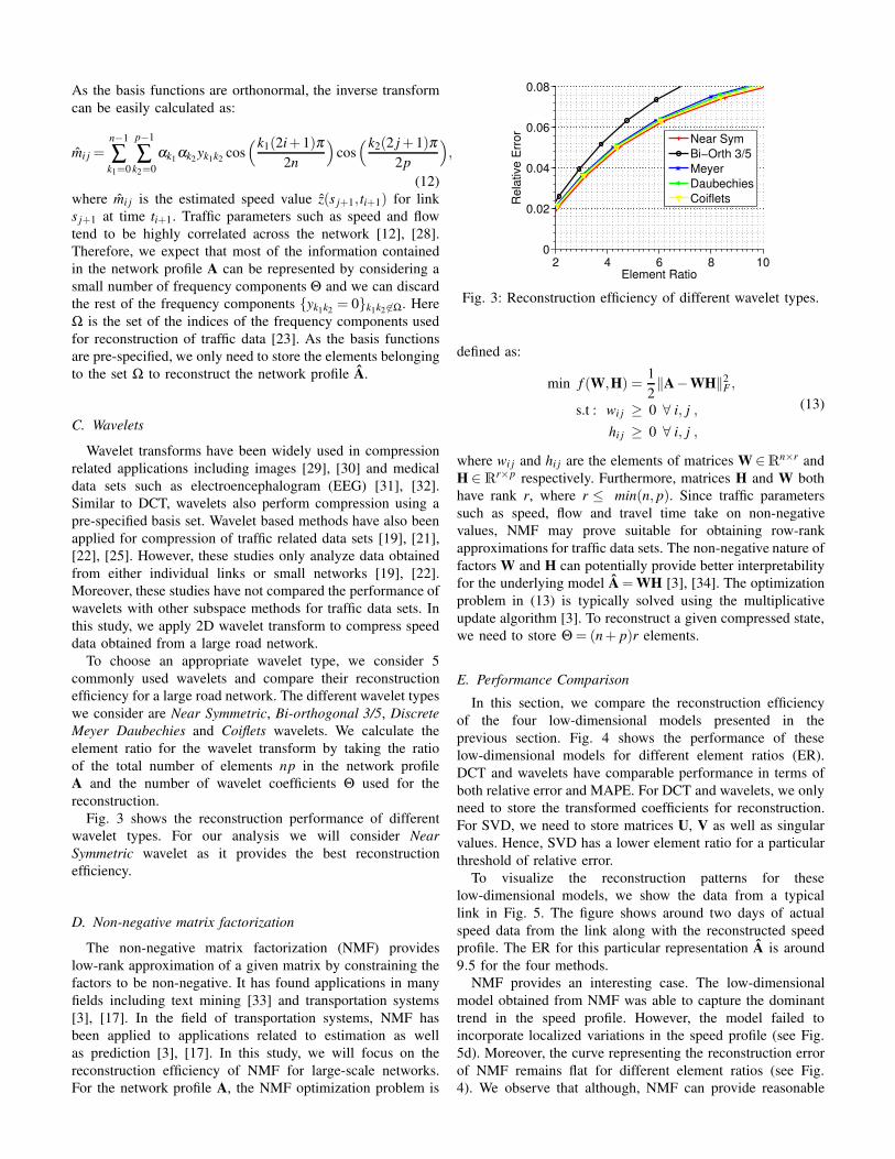
To choose an appropriate wavelet type, we consider 5
commonly used wavelets and compare their reconstruction
efficiency for a large road network. The different wavelet types
we consider are Near Symmetric, Bi-orthogonal 3/5, Discrete
Meyer Daubechies and Coiflets wavelets. We calculate the
element ratio for the wavelet transform by taking the ratio
of the total number of elements np in the network profile
A and the number of wavelet coefficients Θ used for the
reconstruction.
Fig. 3 shows the reconstruction performance of different
wavelet types. For our analysis we will consider Near
Symmetric wavelet as it provides the best reconstruction
efficiency.
D. Non-negative matrix factorization
The non-negative matrix factorization (NMF) provides
low-rank approximation of a given matrix by constraining the
factors to be non-negative. It has found applications in many
fields including text mining [33] and transportation systems
[3], [17]. In the field of transportation systems, NMF has
been applied to applications related to estimation as well
as prediction [3], [17]. In this study, we will focus on the
reconstruction efficiency of NMF for large-scale networks.
For the network profile A, the NMF optimization problem is
2 4 6 8 100
0.02
0.04
0.06
0.08
Element Ratio
Rela
tive E
rror
Near Sym
Bi−Orth 3/5
Meyer
Daubechies
Coiflets
Fig. 3: Reconstruction efficiency of different wavelet types.
defined as:
min f (W,H) =1
2‖A−WH‖2
F ,
s.t : wi j ≥ 0 ∀ i, j ,
hi j ≥ 0 ∀ i, j ,
(13)
where wi j and hi j are the elements of matrices W ∈Rn×r and
H ∈Rr×p respectively. Furthermore, matrices H and W both
have rank r, where r ≤ min(n, p). Since traffic parameters
such as speed, flow and travel time take on non-negative
values, NMF may prove suitable for obtaining row-rank
approximations for traffic data sets. The non-negative nature of
factors W and H can potentially provide better interpretability
for the underlying model A = WH [3], [34]. The optimization
problem in (13) is typically solved using the multiplicative
update algorithm [3]. To reconstruct a given compressed state,
we need to store Θ = (n+ p)r elements.
E. Performance Comparison
In this section, we compare the reconstruction efficiency
of the four low-dimensional models presented in the
previous section. Fig. 4 shows the performance of these
low-dimensional models for different element ratios (ER).
DCT and wavelets have comparable performance in terms of
both relative error and MAPE. For DCT and wavelets, we only
need to store the transformed coefficients for reconstruction.
For SVD, we need to store matrices U, V as well as singular
values. Hence, SVD has a lower element ratio for a particular
threshold of relative error.
To visualize the reconstruction patterns for these
low-dimensional models, we show the data from a typical
link in Fig. 5. The figure shows around two days of actual
speed data from the link along with the reconstructed speed
profile. The ER for this particular representation A is around
9.5 for the four methods.
NMF provides an interesting case. The low-dimensional
model obtained from NMF was able to capture the dominant
trend in the speed profile. However, the model failed to
incorporate localized variations in the speed profile (see Fig.
5d). Moreover, the curve representing the reconstruction error
of NMF remains flat for different element ratios (see Fig.
4). We observe that although, NMF can provide reasonable
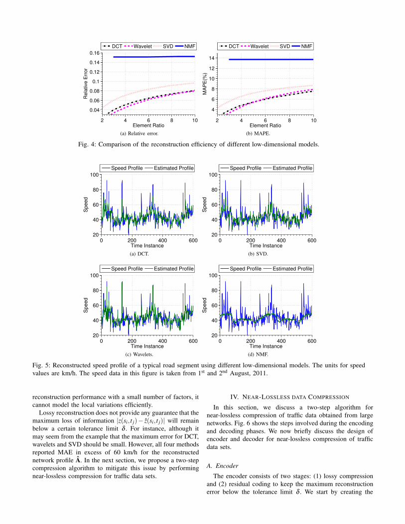
2 4 6 8 10
0.04
0.06
0.08
0.1
0.12
0.14
0.16
Element Ratio
Rela
tive E
rror
DCT Wavelet SVD NMF
(a) Relative error.
2 4 6 8 10
4
6
8
10
12
14
Element Ratio
MA
PE
(%)
DCT Wavelet SVD NMF
(b) MAPE.
Fig. 4: Comparison of the reconstruction efficiency of different low-dimensional models.
0 200 400 60020
40
60
80
100
Time Instance
Sp
ee
d
Speed Profile Estimated Profile
(a) DCT.
0 200 400 60020
40
60
80
100
Time Instance
Sp
ee
d
Speed Profile Estimated Profile
(b) SVD.
0 200 400 60020
40
60
80
100
Time Instance
Sp
ee
d
Speed Profile Estimated Profile
(c) Wavelets.
0 200 400 60020
40
60
80
100
Time Instance
Sp
ee
d
Speed Profile Estimated Profile
(d) NMF.
Fig. 5: Reconstructed speed profile of a typical road segment using different low-dimensional models. The units for speed
values are km/h. The speed data in this figure is taken from 1st and 2nd August, 2011.
reconstruction performance with a small number of factors, it
cannot model the local variations efficiently.
Lossy reconstruction does not provide any guarantee that the
maximum loss of information |z(si, t j)− z(si, t j)| will remain
below a certain tolerance limit δ . For instance, although it
may seem from the example that the maximum error for DCT,
wavelets and SVD should be small. However, all four methods
reported MAE in excess of 60 km/h for the reconstructed
network profile A. In the next section, we propose a two-step
compression algorithm to mitigate this issue by performing
near-lossless compression for traffic data sets.
IV. NEAR-LOSSLESS DATA COMPRESSION
In this section, we discuss a two-step algorithm for
near-lossless compression of traffic data obtained from large
networks. Fig. 6 shows the steps involved during the encoding
and decoding phases. We now briefly discuss the design of
encoder and decoder for near-lossless compression of traffic
data sets.
A. Encoder
The encoder consists of two stages: (1) lossy compression
and (2) residual coding to keep the maximum reconstruction
error below the tolerance limit δ . We start by creating the
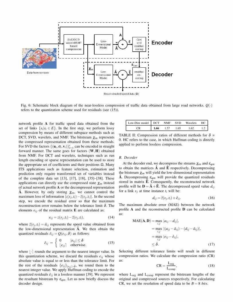
Fig. 6: Schematic block diagram of the near-lossless compression of traffic data obtained from large road networks. Q(·)refers to the quantization scheme used for residuals (see (15)).
network profile A for traffic speed data obtained from the
set of links si|si ∈ E. In the first step, we perform lossy
compression by means of different subspace methods such as
DCT, SVD, wavelets, and NMF. The bitstream χen represents
the compressed representation obtained from these methods.
For SVD the factors (ui,σi,vi)ri=1 can be encoded in straight
forward manner. The same goes for factors (W,H) obtained
from NMF. For DCT and wavelets, techniques such as run
length encoding or sparse representation can be used to store
the appropriate set of coefficients and their positions Ω. Many
ITS applications such as feature selection, estimation and
prediction only require transformed set of variables instead
of the complete data set [13], [17], [18], [35]–[38]. These
applications can directly use the compressed state χen instead
of actual network profile A or the decompressed representation
A. However, by only storing χen, we cannot control the
maximum loss of information |z(s j, ti)− z(s j , ti)|. In the second
step, we encode the residual error so that the maximum
reconstruction error remains below the tolerance limit δ . The
elements ei j of the residual matrix E are calculated as:
ei j = z(s j , ti)− z(s j , ti), (14)
where z(s j, ti) = ai j represents the speed value obtained from
the low-dimensional representation A. We then obtain the
quantized residuals ei j = Q(ei j,δ ) as follows:
ei j =
0 |ei j| ≤ δ⌊ei j⌉ otherwise.
(15)
where ⌊·⌉ rounds the argument to the nearest integer value. In
this quantization scheme, we discard the residuals ei j whose
absolute value is equal to or less than the tolerance limit. For
the rest of the residuals ei j|ei j |>δ , we round them to the
nearest integer value. We apply Huffman coding to encode the
quantized residuals ei j in a lossless manner [39]. We represent
the resultant bitstream by εqen. Let us now briefly discuss the
decoder design.
Low-Dim model DCT NMF SVD Wavelets HC
CR 1.66 1.57 1.65 1.62 1.2
TABLE II: Compression ratios of different methods for δ =
0. HC refers to the case, in which Huffman coding is directly
applied to perform lossless compression.
B. Decoder
At the decoder end, we decompress the streams χen and εqen
to obtain the matrices A and E respectively. Decompressing
the bitstream χen will yield the low-dimensional representation
A. Decompressing εqen will provide the quantized residuals
stored in matrix E. Consequently, the reconstructed network
profile will be D = A+ E. The decompressed speed value di j
for a link s j at time instance ti will be:
di j = z(s j , ti)+ ei j. (16)
The maximum absolute error (MAE) between the network
profile A and the reconstructed profile D can be calculated
as:
MAE(A,D) = maxi, j
|ai j − di j|,
= maxi, j
|(ai j − ai j)− (di j − ai j)|,
= maxi, j
|ei j − ei j|,
≤ δ . (17)
Selecting different tolerance limits will result in different
compression ratios. We calculate the compression ratio (CR)
as:
CR =Lorg
Lcomp, (18)
where Lorg and Lcomp represent the bitstream lengths of the
original and compressed sources respectively. For calculating
CR, we set the resolution of speed data to be B = 8 bits.
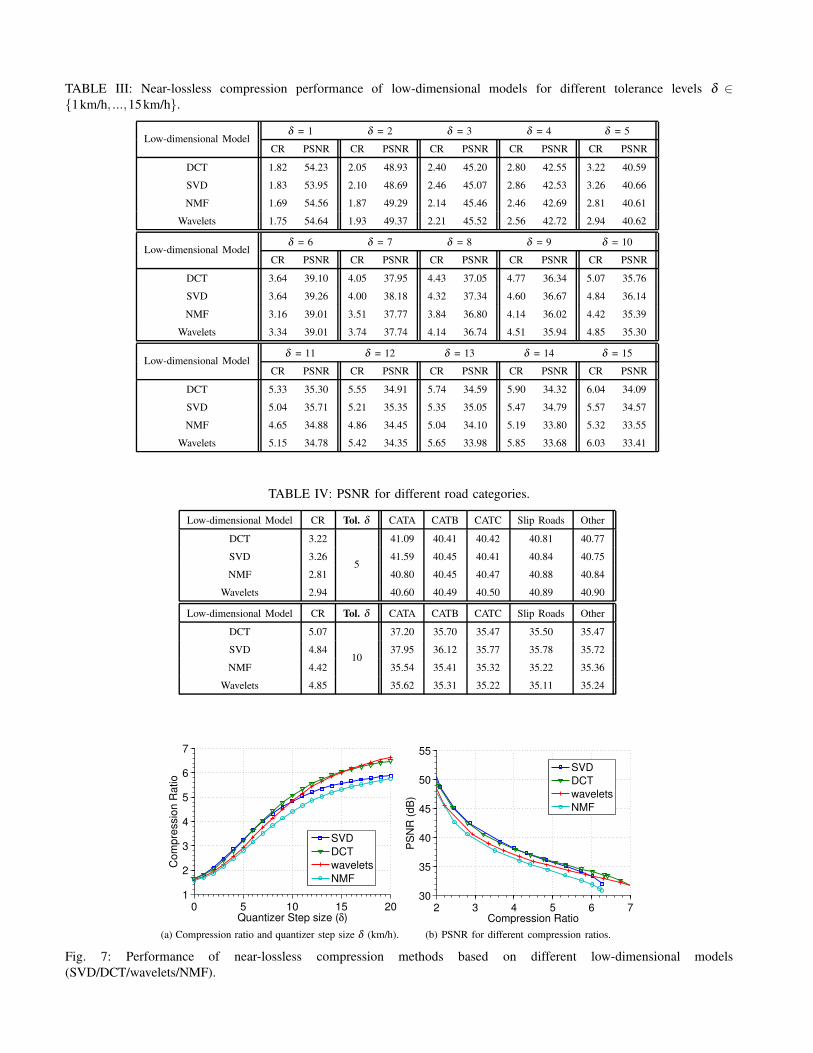
TABLE III: Near-lossless compression performance of low-dimensional models for different tolerance levels δ ∈1km/h, ...,15km/h.
Low-dimensional Modelδ = 1 δ = 2 δ = 3 δ = 4 δ = 5
CR PSNR CR PSNR CR PSNR CR PSNR CR PSNR
DCT 1.82 54.23 2.05 48.93 2.40 45.20 2.80 42.55 3.22 40.59
SVD 1.83 53.95 2.10 48.69 2.46 45.07 2.86 42.53 3.26 40.66
NMF 1.69 54.56 1.87 49.29 2.14 45.46 2.46 42.69 2.81 40.61
Wavelets 1.75 54.64 1.93 49.37 2.21 45.52 2.56 42.72 2.94 40.62
Low-dimensional Modelδ = 6 δ = 7 δ = 8 δ = 9 δ = 10
CR PSNR CR PSNR CR PSNR CR PSNR CR PSNR
DCT 3.64 39.10 4.05 37.95 4.43 37.05 4.77 36.34 5.07 35.76
SVD 3.64 39.26 4.00 38.18 4.32 37.34 4.60 36.67 4.84 36.14
NMF 3.16 39.01 3.51 37.77 3.84 36.80 4.14 36.02 4.42 35.39
Wavelets 3.34 39.01 3.74 37.74 4.14 36.74 4.51 35.94 4.85 35.30
Low-dimensional Modelδ = 11 δ = 12 δ = 13 δ = 14 δ = 15
CR PSNR CR PSNR CR PSNR CR PSNR CR PSNR
DCT 5.33 35.30 5.55 34.91 5.74 34.59 5.90 34.32 6.04 34.09
SVD 5.04 35.71 5.21 35.35 5.35 35.05 5.47 34.79 5.57 34.57
NMF 4.65 34.88 4.86 34.45 5.04 34.10 5.19 33.80 5.32 33.55
Wavelets 5.15 34.78 5.42 34.35 5.65 33.98 5.85 33.68 6.03 33.41
TABLE IV: PSNR for different road categories.
Low-dimensional Model CR Tol. δ CATA CATB CATC Slip Roads Other
DCT 3.22
5
41.09 40.41 40.42 40.81 40.77
SVD 3.26 41.59 40.45 40.41 40.84 40.75
NMF 2.81 40.80 40.45 40.47 40.88 40.84
Wavelets 2.94 40.60 40.49 40.50 40.89 40.90
Low-dimensional Model CR Tol. δ CATA CATB CATC Slip Roads Other
DCT 5.07
10
37.20 35.70 35.47 35.50 35.47
SVD 4.84 37.95 36.12 35.77 35.78 35.72
NMF 4.42 35.54 35.41 35.32 35.22 35.36
Wavelets 4.85 35.62 35.31 35.22 35.11 35.24
0 5 10 15 201
2
3
4
5
6
7
Quantizer Step size (δ)
Com
pre
ssio
n R
atio
SVD
DCT
wavelets
NMF
(a) Compression ratio and quantizer step size δ (km/h).
2 3 4 5 6 730
35
40
45
50
55
Compression Ratio
PS
NR
(dB
)
SVD
DCT
wavelets
NMF
(b) PSNR for different compression ratios.
Fig. 7: Performance of near-lossless compression methods based on different low-dimensional models
(SVD/DCT/wavelets/NMF).
In the next section, we analyze the performance of
the proposed near-lossless compression method for different
tolerance limits.
V. RESULTS AND DISCUSSION
In this section, we analyze the performance of the proposed
algorithms for the test network. We also compare the
compression efficiency of these algorithms for different road
categories, weekdays, and weekends. All the compression
ratios are calculated by keeping the resolution of field data
to B = 8 bits. Considering higher resolution for field data
will automatically result in higher albeit inflated CR. Table II
shows the compression ratios for different subspace methods
by setting δ = 0. If we ignore the rounding off error due to
(15), then this scenario can be considered as the lossless case.
If we directly apply Huffman coding (HC) on the network
profile A, we obtain a CR of 1.2. Hence, the two step
compression method straight away provides around 30 % to
38 % (CR: 1.57− 1.66) improvement in CR. Table III shows
the CR and PSNR achieved by the four low-dimensional
models for different tolerance levels. For tolerance level of
5 km/h, the algorithms yield a CR of around 3. In this case,
the SVD based method provides the highest compression ratio
and PSNR. The other three methods also report similar PSNR.
DCT has comparable CR to that of SVD. The other two
methods (wavelets and NMF) report slightly smaller CR for
this particular tolerance level. For tolerance level of 15 km/h,
DCT and wavelets achieve CR of more than 6 (see Table
III). While SVD has the best PSNR for this tolerance level, it
reports slightly smaller CR (5.57) as compared to DCT (6.04)
and wavelets (6.03).
To observe these trends in more detail, we plot the
compression ratios achieved by these algorithms against
different tolerance levels in Fig. 7a. All the algorithms report
similar CR for tolerance levels close to zero. For higher
tolerance levels, DCT and wavelets achieve higher CR as
compared to matrix decomposition methods (SVD, NMF). For
low tolerance levels, residual coding can easily compensate
for the inefficiency of a particular low-dimensional model.
For higher CR, such inefficiencies become prominent. The
tolerance level (MAE) alone does not provide all the
information about the overall reconstruction error. Two
methods with the same MAE can still have different mean
square error. To this end, we plot PSNR against the
compression ratios for these methods. PSNR values for
different compression ratios are shown in Fig. 7b. The plot
shows that SVD provides similar PSNR to DCT for a given
CR. However, SVD yields higher maximum error as compared
to DCT (see Fig. 7a).
Table IV shows the category wise analysis of different
near-lossless compression methods for tolerance levels of 5
km/h and 10 km/h. Expressways (CATA roads) achieve higher
PSNR as compared to roads from CATB and CATC for all
four algorithms. This difference in PSNR is more visible for
δ = 10 as opposed to δ = 5. For δ = 10 , expressways have the
highest PSNR in comparison with CATB, CATC, slip roads
and other categories for each algorithm. Nonetheles, the PSNR
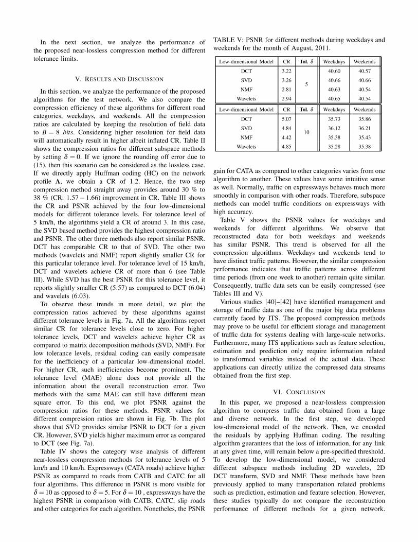
TABLE V: PSNR for different methods during weekdays and
weekends for the month of August, 2011.
Low-dimensional Model CR Tol. δ Weekdays Weekends
DCT 3.22
5
40.60 40.57
SVD 3.26 40.66 40.66
NMF 2.81 40.63 40.54
Wavelets 2.94 40.65 40.54
Low-dimensional Model CR Tol. δ Weekdays Weekends
DCT 5.07
10
35.73 35.86
SVD 4.84 36.12 36.21
NMF 4.42 35.38 35.43
Wavelets 4.85 35.28 35.38
gain for CATA as compared to other categories varies from one
algorithm to another. These values have some intuitive sense
as well. Normally, traffic on expressways behaves much more
smoothly in comparison with other roads. Therefore, subspace
methods can model traffic conditions on expressways with
high accuracy.
Table V shows the PSNR values for weekdays and
weekends for different algorithms. We observe that
reconstructed data for both weekdays and weekends
has similar PSNR. This trend is observed for all the
compression algorithms. Weekdays and weekends tend to
have distinct traffic patterns. However, the similar compression
performance indicates that traffic patterns across different
time periods (from one week to another) remain quite similar.
Consequently, traffic data sets can be easily compressed (see
Tables III and V).
Various studies [40]–[42] have identified management and
storage of traffic data as one of the major big data problems
currently faced by ITS. The proposed compression methods
may prove to be useful for efficient storage and management
of traffic data for systems dealing with large-scale networks.
Furthermore, many ITS applications such as feature selection,
estimation and prediction only require information related
to transformed variables instead of the actual data. These
applications can directly utilize the compressed data streams
obtained from the first step.
VI. CONCLUSION
In this paper, we proposed a near-lossless compression
algorithm to compress traffic data obtained from a large
and diverse network. In the first step, we developed
low-dimensional model of the network. Then, we encoded
the residuals by applying Huffman coding. The resulting
algorithm guarantees that the loss of information, for any link
at any given time, will remain below a pre-specified threshold.
To develop the low-dimensional model, we considered
different subspace methods including 2D wavelets, 2D
DCT transform, SVD and NMF. These methods have been
previously applied to many transportation related problems
such as prediction, estimation and feature selection. However,
these studies typically do not compare the reconstruction
performance of different methods for a given network.
In this study, we analyzed the reconstruction efficiency
of different subspace methods for a large and diverse
network which consisted of more than 18000 road segments.
We then applied these methods to perform near-lossless
compression of the speed data. We also analyzed the
performance of the proposed algorithm for different road
categories, weekdays and weekends by considering different
low-dimensional methods. We conclude that low-dimensional
based near-lossless compression methods can efficiently
compress traffic data sets obtained from large and diverse road
networks.
ACKNOWLEDGMENT
This work was supported in part by the Singapore National
Research Foundation through the Singapore Massachusetts
Institute of Technology Alliance for Research and Technology
(SMART) Center for Future Mobility (FM).
LIST OF ABBREVIATIONS
CR Compression ratio
DCT Discrete cosine transform
EEG Electroencephalogram
ER Element ratios
HC Huffman coding
ITS Intelligent transportation systems
LTA Land transportation authority
MAE Maximum absolute error
MAPE Mean absolute percentage error
MSE Mean square error
NMF Non-negative matrix factorization
PCA Principal component analysis
PSNR Peak signal-to-noise ratio
SVD Singular value decomposition
REFERENCES
[1] J. Zhang, F.-Y. Wang, K. Wang, W.-H. Lin, X. Xu, and C. Chen,“Data-driven intelligent transportation systems: A survey,” Intelligent
Transportation Systems, IEEE Transactions on, vol. 12, no. 4, pp.1624–1639, 2011.
[2] P. J. Bickel, C. Chen, J. Kwon, J. Rice, E. Van Zwet, and P. Varaiya,“Measuring traffic,” Statistical Science, vol. 22, no. 4, pp. 581–597,2007.
[3] A. Hofleitner, R. Herring, A. Bayen, Y. Han, F. Moutarde, andA. de La Fortelle, “Large-scale estimation of arterial traffic and structuralanalysis of traffic patterns from probe vehicles,” in Transportation
Research Board 91st Annual Meeting, no. 12-0598, 2012.[4] M. T. Asif, N. Mitrovic, L. Garg, J. Dauwels, and P. Jaillet,
“Low-dimensional models for missing data imputation in roadnetworks,” in Acoustics, Speech and Signal Processing (ICASSP), 2013
IEEE International Conference on, 2013, pp. 3527–3531.[5] S. Reddy, M. Mun, J. Burke, D. Estrin, M. Hansen, and M. Srivastava,
“Using mobile phones to determine transportation modes,” ACM
Transactions on Sensor Networks (TOSN), vol. 6, no. 2, p. 13, 2010.[6] A. Hofleitner, R. Herring, P. Abbeel, and A. Bayen, “Learning the
dynamics of arterial traffic from probe data using a dynamic bayesiannetwork,” Intelligent Transportation Systems, IEEE Transactions on,vol. 13, no. 4, pp. 1679–1693, 2012.
[7] W. Min and L. Wynter, “Real-time road traffic prediction withspatio-temporal correlations,” Transportation Research Part C:
Emerging Technologies, vol. 19, no. 4, pp. 606–616, 2011.[8] M. T. Asif, J. Dauwels, C. Y. Goh, A. Oran, E. Fathi, M. Xu, M. Dhanya,
N. Mitrovic, and P. Jaillet, “Spatiotemporal patterns in large-scale trafficspeed prediction,” Intelligent Transportation Systems, IEEE Transactions
on, vol. 15, no. 2, pp. 794–804, April 2014.
[9] C. Y. Goh, J. Dauwels, N. Mitrovic, M. T. Asif, A. Oran, andP. Jaillet, “Online map-matching based on hidden markov model forreal-time traffic sensing applications,” in Intelligent Transportation
Systems (ITSC), 2012 15th International IEEE Conference on, 2012,pp. 776–781.
[10] Z. Li, Y. Zhu, H. Zhu, and M. Li, “Compressive sensing approach tourban traffic sensing,” in Distributed Computing Systems (ICDCS), 2011
31st International Conference on, 2011, pp. 889–898.
[11] L. Li, D. Wen, and D. Yao, “A survey of traffic control with vehicularcommunications,” Intelligent Transportation Systems, IEEE Transactions
on, vol. PP, no. 99, pp. 1–8, 2013.
[12] L. Qu, L. Li, Y. Zhang, and J. Hu, “Ppca-based missing dataimputation for traffic flow volume: A systematical approach,” Intelligent
Transportation Systems, IEEE Transactions on, vol. 10, no. 3, pp.512–522, 2009.
[13] T. Djukic, G. Flotterod, H. van Lint, and S. Hoogendoorn, “Efficientreal time od matrix estimation based on principal component analysis,”in Intelligent Transportation Systems (ITSC), 2012 15th International
IEEE Conference on. IEEE, 2012, pp. 115–121.
[14] R. Herring, A. Hofleitner, P. Abbeel, and A. Bayen, “Estimating arterialtraffic conditions using sparse probe data,” in Intelligent Transportation
Systems (ITSC), 2010 13th International IEEE Conference on. IEEE,2010, pp. 929–936.
[15] J. Ribeiro Junior, M. Mitre Campista, and L. Costa, “Cotrams: Acollaborative and opportunistic traffic monitoring system,” Intelligent
Transportation Systems, IEEE Transactions on, vol. 15, no. 3, pp.949–958, June 2014.
[16] J. Rodrigues, A. Aguiar, F. Vieira, J. Barros, and J. P. S. Cunha,“A mobile sensing architecture for massive urban scanning,” inIntelligent Transportation Systems (ITSC), 2011 14th International IEEE
Conference on, Oct 2011, pp. 1132–1137.
[17] Y. Han and F. Moutarde, “Analysis of network-level traffic statesusing locality preservative non-negative matrix factorization,” inIntelligent Transportation Systems (ITSC), 2011 14th International IEEE
Conference on. IEEE, 2011, pp. 501–506.
[18] C. Furtlehner, Y. Han, J.-M. Lasgouttes, V. Martin, F. Marchal, andF. Moutarde, “Spatial and temporal analysis of traffic states on largescale networks,” in Intelligent Transportation Systems (ITSC), 2010 13th
International IEEE Conference on. IEEE, 2010, pp. 1215–1220.
[19] Y. Xiao, Y.-m. Xie, L. Lu, and S. Gao, “The traffic data compression anddecompression for intelligent traffic systems based on two-dimensionalwavelet transformation,” in Signal Processing, 2004. Proceedings.
ICSP’04. 2004 7th International Conference on, vol. 3. IEEE, 2004,pp. 2560–2563.
[20] Q. Li, H. Jianming, and Z. Yi, “A flow volumes data compressionapproach for traffic network based on principal component analysis,” inIntelligent Transportation Systems Conference, 2007. ITSC 2007. IEEE.IEEE, 2007, pp. 125–130.
[21] X.-f. Shi and L.-l. Liang, “A data compression method for trafficloop detectors’ signals based on lifting wavelet transformation andentropy coding,” in Information Science and Engineering (ISISE), 2010
International Symposium on. IEEE, 2010, pp. 129–132.
[22] J. Ding, Z. Zhang, and X. Ma, “A method for urban traffic datacompression based on wavelet-pca,” in Computational Sciences and
Optimization (CSO), 2011 Fourth International Joint Conference on.IEEE, 2011, pp. 1030–1034.
[23] M. T. Asif, S. Kannan, J. Dauwels, and P. Jaillet, “Data compressiontechniques for urban traffic data,” in Computational Intelligence in
Vehicles and Transportation Systems (CIVTS), 2013 IEEE Symposium
on, 2013, pp. 44–49.
[24] G. Ke, J. Hu, L. He, and Z. Li, “Data reduction in urban traffic sensornetwork,” in Intelligent Vehicles Symposium, 2009 IEEE, June 2009, pp.1021–1026.
[25] F. Qiao, H. Liu, and L. Yu, “Incorporating wavelet decompositiontechnique to compress transguide intelligent transportation system data,”Transportation Research Record: Journal of the Transportation Research
Board, vol. 1968, no. 1, pp. 63–74, 2006.
[26] ——, “Intelligent transportation systems data compression using waveletdecomposition technique,” Tech. Rep., 2009.
[27] N. Thomos, N. V. Boulgouris, and M. G. Strintzis, “Optimizedtransmission of jpeg2000 streams over wireless channels,” Image
Processing, IEEE Transactions on, vol. 15, no. 1, pp. 54–67, 2006.
[28] T. Djukic, J. van Lint, and S. Hoogendoorn, “Exploring applicationperspectives of principal component analysis in predicting dynamicorigin-destination matrices,” in Transportation Research Board 91st
Annual Meeting, no. 12-2702, 2012.
[29] M. Antonini, M. Barlaud, P. Mathieu, and I. Daubechies, “Image codingusing wavelet transform,” Image Processing, IEEE Transactions on,vol. 1, no. 2, pp. 205–220, 1992.
[30] R. W. Buccigrossi and E. P. Simoncelli, “Image compression via jointstatistical characterization in the wavelet domain,” Image Processing,
IEEE Transactions on, vol. 8, no. 12, pp. 1688–1701, 1999.[31] K. Srinivasan, J. Dauwels, and M. Reddy, “Multichannel EEG
compression: Wavelet-based image and volumetric coding approach,”Biomedical and Health Informatics, IEEE Journal of, vol. 17, no. 1, pp.113–120, 2013.
[32] J. Dauwels, K. Srinivasan, M. Reddy, and A. Cichocki, “Near-losslessmultichannel EEG compression based on matrix and tensordecompositions,” Biomedical and Health Informatics, IEEE Journal of,vol. 17, no. 3, pp. 708–714, 2013.
[33] M. W. Berry, M. Browne, A. N. Langville, V. P. Pauca, and R. J.Plemmons, “Algorithms and applications for approximate nonnegativematrix factorization,” Computational Statistics & Data Analysis, vol. 52,no. 1, pp. 155–173, 2007.
[34] D. Donoho and V. Stodden, “When does non-negative matrixfactorization give a correct decomposition into parts?” in Advances in
Neural Information Processing Systems, 2004, pp. 1141–1148.[35] X. Jin, Y. Zhang, and D. Yao, “Simultaneously prediction of network
traffic flow based on pca-svr,” in Advances in Neural Networks–ISNN
2007. Springer, 2007, pp. 1022–1031.[36] T. T. Tchrakian, B. Basu, and M. O’Mahony, “Real-time traffic flow
forecasting using spectral analysis,” Intelligent Transportation Systems,
IEEE Transactions on, vol. 13, no. 2, pp. 519–526, 2012.[37] X. Jiang and H. Adeli, “Dynamic wavelet neural network model for
traffic flow forecasting,” Journal of Transportation Engineering, vol.131, no. 10, pp. 771–779, 2005.
[38] Y. Zhang, Y. Zhang, and A. Haghani, “A hybrid short-term traffic flowforecasting method based on spectral analysis and statistical volatilitymodel,” Transportation Research Part C: Emerging Technologies, 2013.
[39] K. Sayood, Introduction to data compression. Access Online viaElsevier, 2012.
[40] T. Qu, S. T. Parker, Y. Cheng, B. Ran, and D. A. Noyce, “Large-scaleintelligent transportation system traffic detector data archiving,” inTransportation Research Board 93rd Annual Meeting, no. 14-5448,2014.
[41] I. Vilajosana, J. Llosa, B. Martinez, M. Domingo-Prieto, A. Angles, andX. Vilajosana, “Bootstrapping smart cities through a self-sustainablemodel based on big data flows,” Communications Magazine, IEEE,vol. 51, no. 6, pp. 128–134, June 2013.
[42] H. Jagadish, J. Gehrke, A. Labrinidis, Y. Papakonstantinou, J. M.Patel, R. Ramakrishnan, and C. Shahabi, “Big data and its technicalchallenges,” Communications of the ACM, vol. 57, no. 7, pp. 86–94,2014.
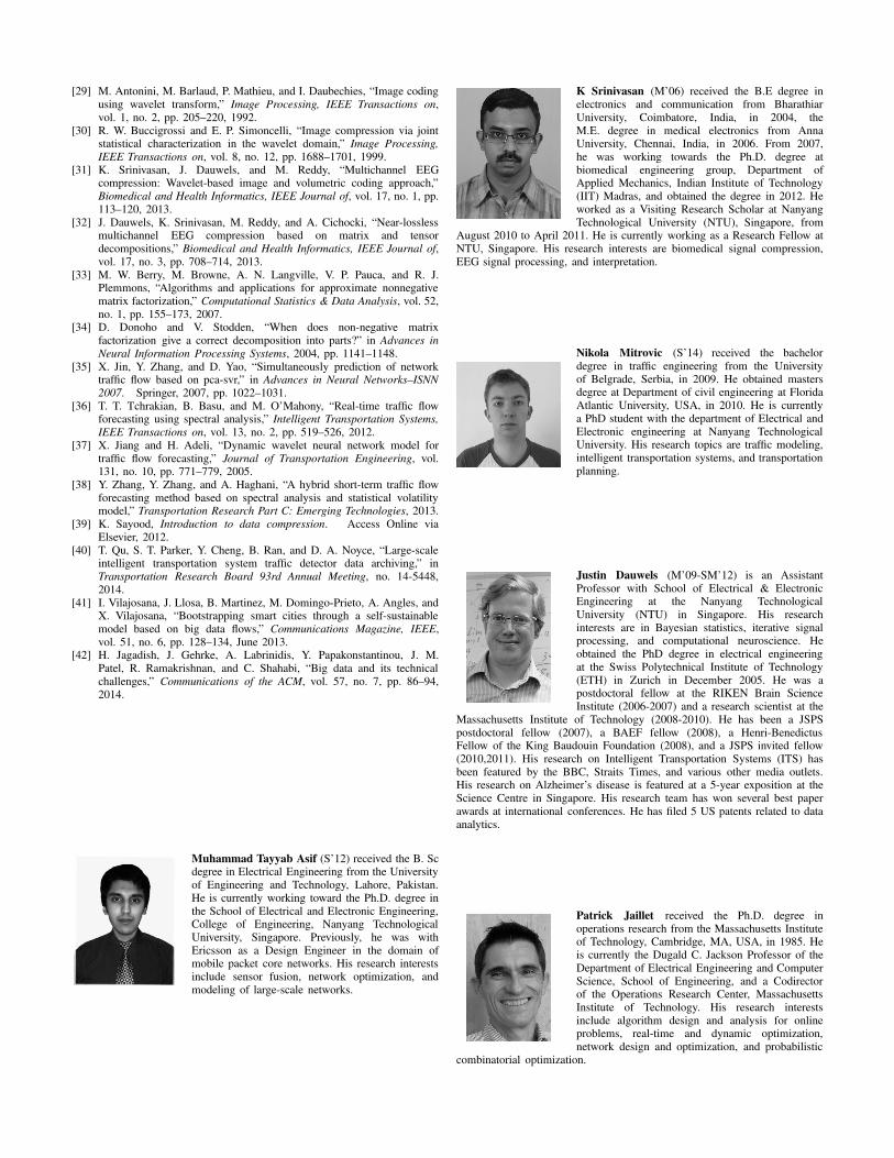
Muhammad Tayyab Asif (S’12) received the B. Scdegree in Electrical Engineering from the Universityof Engineering and Technology, Lahore, Pakistan.He is currently working toward the Ph.D. degree inthe School of Electrical and Electronic Engineering,College of Engineering, Nanyang TechnologicalUniversity, Singapore. Previously, he was withEricsson as a Design Engineer in the domain ofmobile packet core networks. His research interestsinclude sensor fusion, network optimization, andmodeling of large-scale networks.
K Srinivasan (M’06) received the B.E degree inelectronics and communication from BharathiarUniversity, Coimbatore, India, in 2004, theM.E. degree in medical electronics from AnnaUniversity, Chennai, India, in 2006. From 2007,he was working towards the Ph.D. degree atbiomedical engineering group, Department ofApplied Mechanics, Indian Institute of Technology(IIT) Madras, and obtained the degree in 2012. Heworked as a Visiting Research Scholar at NanyangTechnological University (NTU), Singapore, from
August 2010 to April 2011. He is currently working as a Research Fellow atNTU, Singapore. His research interests are biomedical signal compression,EEG signal processing, and interpretation.
Nikola Mitrovic (S’14) received the bachelordegree in traffic engineering from the Universityof Belgrade, Serbia, in 2009. He obtained mastersdegree at Department of civil engineering at FloridaAtlantic University, USA, in 2010. He is currentlya PhD student with the department of Electrical andElectronic engineering at Nanyang TechnologicalUniversity. His research topics are traffic modeling,intelligent transportation systems, and transportationplanning.
Justin Dauwels (M’09-SM’12) is an AssistantProfessor with School of Electrical & ElectronicEngineering at the Nanyang TechnologicalUniversity (NTU) in Singapore. His researchinterests are in Bayesian statistics, iterative signalprocessing, and computational neuroscience. Heobtained the PhD degree in electrical engineeringat the Swiss Polytechnical Institute of Technology(ETH) in Zurich in December 2005. He was apostdoctoral fellow at the RIKEN Brain ScienceInstitute (2006-2007) and a research scientist at the
Massachusetts Institute of Technology (2008-2010). He has been a JSPSpostdoctoral fellow (2007), a BAEF fellow (2008), a Henri-BenedictusFellow of the King Baudouin Foundation (2008), and a JSPS invited fellow(2010,2011). His research on Intelligent Transportation Systems (ITS) hasbeen featured by the BBC, Straits Times, and various other media outlets.His research on Alzheimer’s disease is featured at a 5-year exposition at theScience Centre in Singapore. His research team has won several best paperawards at international conferences. He has filed 5 US patents related to dataanalytics.
Patrick Jaillet received the Ph.D. degree inoperations research from the Massachusetts Instituteof Technology, Cambridge, MA, USA, in 1985. Heis currently the Dugald C. Jackson Professor of theDepartment of Electrical Engineering and ComputerScience, School of Engineering, and a Codirectorof the Operations Research Center, MassachusettsInstitute of Technology. His research interestsinclude algorithm design and analysis for onlineproblems, real-time and dynamic optimization,network design and optimization, and probabilistic
combinatorial optimization.