NE 455L/491 Nanomaterials Lab Report - Rajesh...

NE 455L/491 Nanomaterials Lab Report

University of Waterloo

4B Nanotechnology Engineering

Group 7

Rajesh Swaminathan

Student ID: 20194189

Email: [email protected]

Phone: 519-590-5439

Lab Partner: Peter Lee (20201956)

Dates Lab Performed On: Jan 28, Feb 4, Feb 11 2010

Lab Report Submitted on Feb 17 2010

Lab Instructor: Aiping Yu

2

Lab 4 Production of a SWNT/PDMS Nanocomposite

Introduction and Objective

The objective of this laboratory experiment is to produce dog bones of a composite material

made of PDMS homogenously interspersed with SWNTs. The electrical conductivity of these

dog bones will be determined using 2-point and 4-point probes. With these conductivity values,

we will be able to determine the relationship between the nanocomposite’s electrical

conductivity and the SWNT loading percentage. Homogenous dispersion of the SWNTs in the

PDMS matrix will be achieved using an ultrasonic disperser and high shear mixing using an

electrical homogenizer.

Experimental Procedure

The procedure for this laboratory was obtained from the NE 455L/491L Nanomaterials

Laboratory 4 part of the Nanotechnology Engineering Program 4B Lab Manuals, 2010. No

deviations were observed.

Discussion and Analysis of Data

We were Group B. We had a CNT percentage weight loading of 1.5%. We therefore added

0.1675g of SWCNT to form our polymer composite matrix.

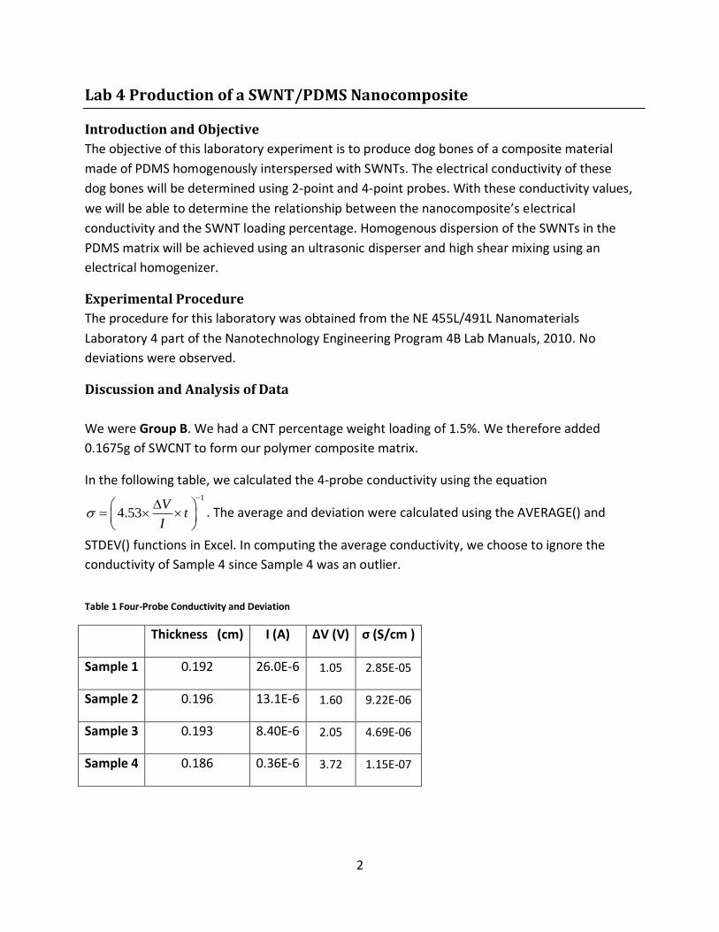
In the following table, we calculated the 4-probe conductivity using the equation 1

4.53V

tI

. The average and deviation were calculated using the AVERAGE() and

STDEV() functions in Excel. In computing the average conductivity, we choose to ignore the

conductivity of Sample 4 since Sample 4 was an outlier.

Table 1 Four-Probe Conductivity and Deviation

Thickness (cm) I (A) ∆V (V) σ (S/cm )

Sample 1 0.192 26.0E-6 1.05 2.85E-05

Sample 2 0.196 13.1E-6 1.60 9.22E-06

Sample 3 0.193 8.40E-6 2.05 4.69E-06

Sample 4 0.186 0.36E-6 3.72 1.15E-07

3

∑σ/4 (S/cm) Deviation

1.41E-05 1.26E-05

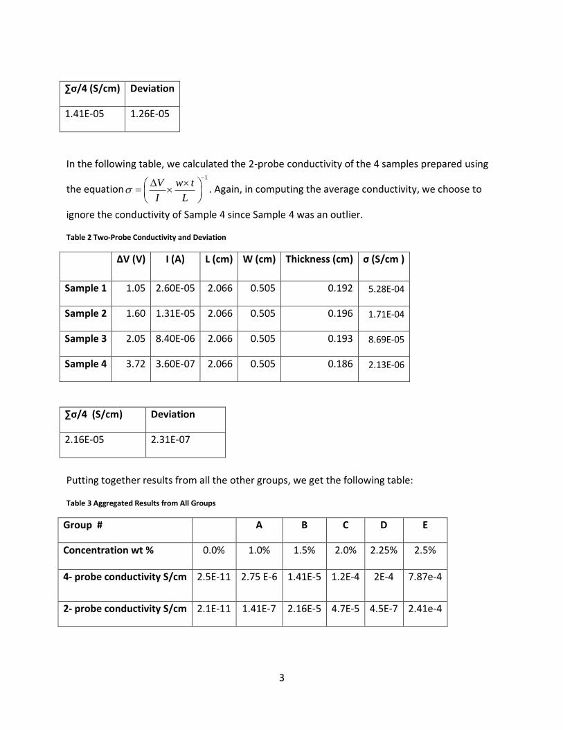
In the following table, we calculated the 2-probe conductivity of the 4 samples prepared using

the equation1

V w t

I L

. Again, in computing the average conductivity, we choose to

ignore the conductivity of Sample 4 since Sample 4 was an outlier.

Table 2 Two-Probe Conductivity and Deviation

∆V (V) I (A) L (cm) W (cm) Thickness (cm) σ (S/cm )

Sample 1 1.05 2.60E-05 2.066 0.505 0.192 5.28E-04

Sample 2 1.60 1.31E-05 2.066 0.505 0.196 1.71E-04

Sample 3 2.05 8.40E-06 2.066 0.505 0.193 8.69E-05

Sample 4 3.72 3.60E-07 2.066 0.505 0.186 2.13E-06

∑σ/4 (S/cm) Deviation

2.16E-05 2.31E-07

Putting together results from all the other groups, we get the following table:

Table 3 Aggregated Results from All Groups

Group # A B C D E

Concentration wt % 0.0% 1.0% 1.5% 2.0% 2.25% 2.5%

4- probe conductivity S/cm 2.5E-11 2.75 E-6 1.41E-5 1.2E-4 2E-4 7.87e-4

2- probe conductivity S/cm 2.1E-11 1.41E-7 2.16E-5 4.7E-5 4.5E-7 2.41e-4

4

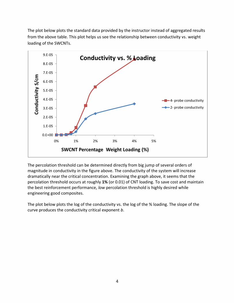
The plot below plots the standard data provided by the instructor instead of aggregated results

from the above table. This plot helps us see the relationship between conductivity vs. weight

loading of the SWCNTs.

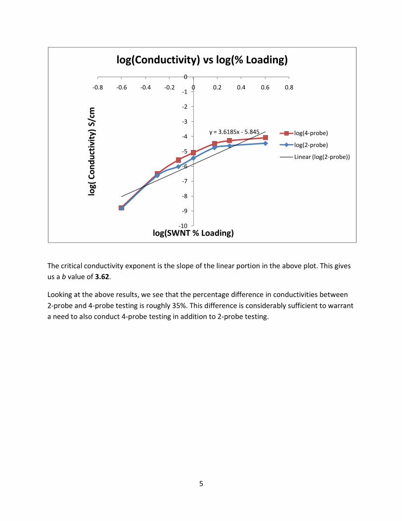
The percolation threshold can be determined directly from big jump of several orders of magnitude in conductivity in the figure above. The conductivity of the system will increase dramatically near the critical concentration. Examining the graph above, it seems that the percolation threshold occurs at roughly 1% (or 0.01) of CNT loading. To save cost and maintain the best reinforcement performance, low percolation threshold is highly desired while engineering good composites. The plot below plots the log of the conductivity vs. the log of the % loading. The slope of the curve produces the conductivity critical exponent b.

0.E+00

1.E-05

2.E-05

3.E-05

4.E-05

5.E-05

6.E-05

7.E-05

8.E-05

9.E-05

0% 1% 2% 3% 4% 5%

Co

nd

uct

ivit

y S/

cm

SWCNT Percentage Weight Loading (%)

Conductivity vs. % Loading

4- probe conductivity

2- probe conductivity

5

The critical conductivity exponent is the slope of the linear portion in the above plot. This gives

us a b value of 3.62.

Looking at the above results, we see that the percentage difference in conductivities between

2-probe and 4-probe testing is roughly 35%. This difference is considerably sufficient to warrant

a need to also conduct 4-probe testing in addition to 2-probe testing.

y = 3.6185x - 5.845

-10

-9

-8

-7

-6

-5

-4

-3

-2

-1

0

-0.8 -0.6 -0.4 -0.2 0 0.2 0.4 0.6 0.8lo

g( C

on

du

ctiv

ity)

S/c

m

log(SWNT % Loading)

log(Conductivity) vs log(% Loading)

log(4-probe)

log(2-probe)

Linear (log(2-probe))

6

Lab 5 Ionic Polymer Actuator


An actuator is a device that converts electrical energy to mechanical energy. The objective of

this lab is to fabricate a specific kind of actuator, known as an ionic polymer actuator (IPA) that

uses material response to achieve actuation under a time-varying electric field. The electrical

and mechanical properties of this IPA actuator will then be characterized and analyzed for the

use of biomimetic actuators. At the end of the laboratory experiment, all the fundamental laws

behind electrical actuation of IPAs will be understood.

Ionic polymer actuators operate under low voltages and can be used in prosthetic devices and

microscopic pumps. The ionic polymer used in this lab will be Nafion in a composite matrix with

carbon nanotubes. Sudden migration of ions causes deformation in the structure, and this

uneven deformation leads to bending of the sheet.



Laboratory 5 part of the Nanotechnology Engineering Program 4B Lab Manuals, 2010. No

deviations were observed.


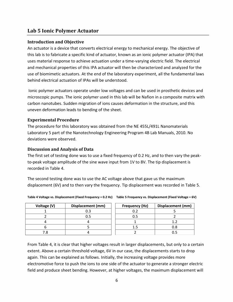
The first set of testing done was to use a fixed frequency of 0.2 Hz, and to then vary the peak-

to-peak voltage amplitude of the sine wave input from 1V to 8V. The tip displacement is

recorded in Table 4.

The second testing done was to use the AC voltage above that gave us the maximum

displacement (6V) and to then vary the frequency. Tip displacement was recorded in Table 5.

Table 4 Voltage vs. Displacement (Fixed Frequency = 0.2 Hz) Table 5 Frequency vs. Displacement (Fixed Voltage = 6V)

Voltage (V) Displacement (mm)

1 0.3

2 0.5

4 4

6 5

7.8 4

From Table 4, it is clear that higher voltages result in larger displacements, but only to a certain

extent. Above a certain threshold voltage, 6V in our case, the displacements starts to drop

again. This can be explained as follows. Initially, the increasing voltage provides more

electromotive force to push the ions to one side of the actuator to generate a stronger electric

field and produce sheet bending. However, at higher voltages, the maximum displacement will

Frequency (Hz) Displacement (mm)

0.2 5

0.5 2

1 1.2

1.5 0.8

2 0.5

7

have been achieved since all ions will have already migrated to one side of the actuator. Any

excess voltage applied will not help the ions move any further and will only lead to reduced

displacement.

From Table 5, we see that higher voltage frequencies result in lower displacements. This is

because at higher frequencies, the actuators do not have sufficient time to achieve their full

mechanical response to the electrical field. The ions are therefore mostly contained within the

polymer. At low frequencies however, the actuator has sufficient time to reach its full

displacement at the most optimal voltage. The water and hydrated ions have more than

enough time to rush out of the surface electrodes. Hence, tip displacements decreases with an

increase in frequency.

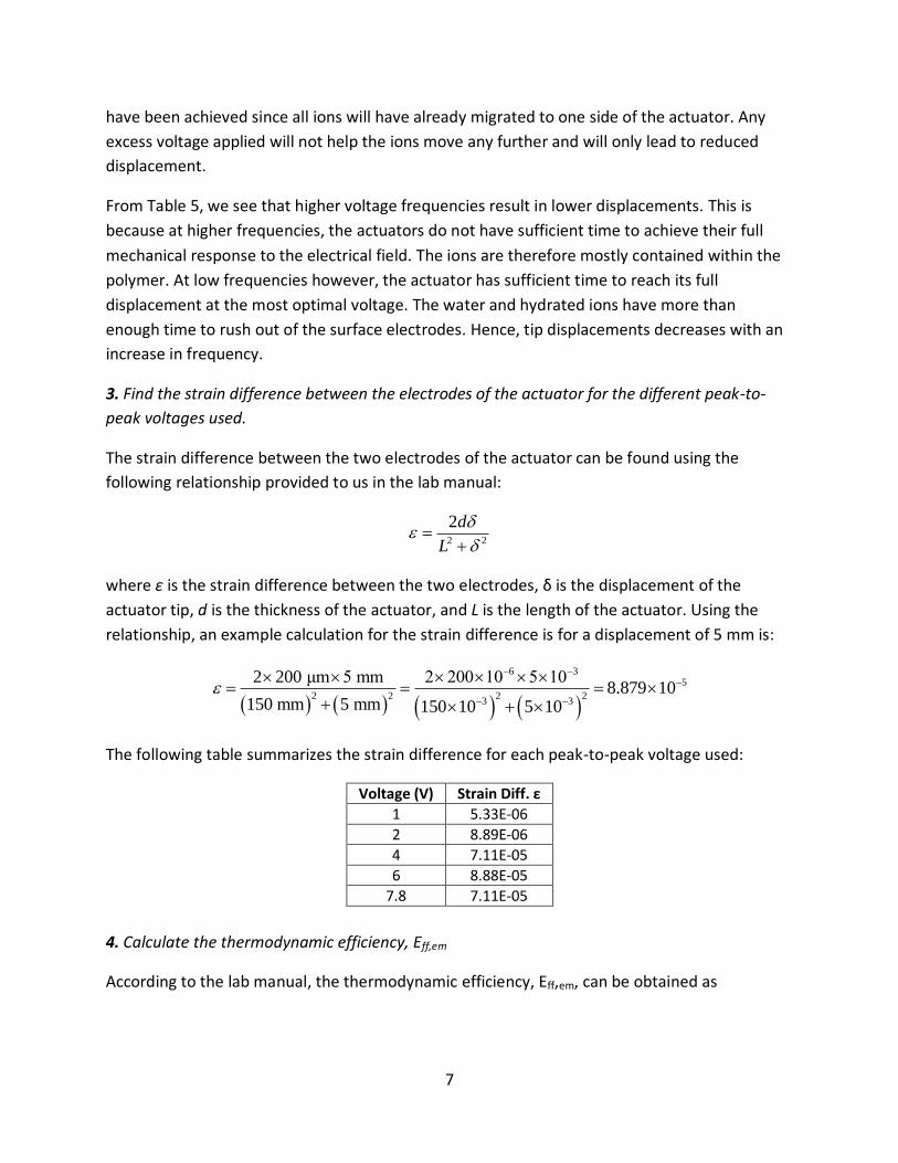
3. Find the strain difference between the electrodes of the actuator for the different peak-to-

peak voltages used.

The strain difference between the two electrodes of the actuator can be found using the

following relationship provided to us in the lab manual:

22

2

L

d

where ε is the strain difference between the two electrodes, δ is the displacement of the

actuator tip, d is the thickness of the actuator, and L is the length of the actuator. Using the

relationship, an example calculation for the strain difference is for a displacement of 5 mm is:

6 35

2 2 2 23 3

2 200 μm 5 mm 2 200 10 5 108.879 10

150 mm 5 mm 150 10 5 10

The following table summarizes the strain difference for each peak-to-peak voltage used:

Voltage (V) Strain Diff. ε

1 5.33E-06

2 8.89E-06

4 7.11E-05

6 8.88E-05

7.8 7.11E-05

4. Calculate the thermodynamic efficiency, Eff,em

According to the lab manual, the thermodynamic efficiency, Eff,em, can be obtained as

8

100(%), in

outemff

P

PE

where Pin is the electrical power input to the IPA. The input power Pin can be calculated using 2V

R. The resistance of the actuator can be calculated from the resistance using

LR

A

, where

ρ is the resistivity of the film (1.3E7 Ω.cm for a 2.5 wt% CNT Nafion film). The cross-sectional

area A of the actuator is just the width times the thickness. The output power Pout is F f ,

where F is the force on the actuator, δ is the tip displacement and f is the input frequency.

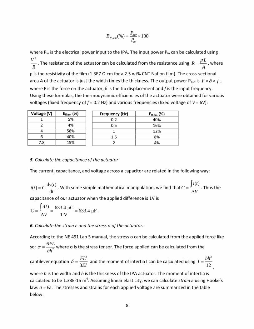
Using these formulas, the thermodynamic efficiencies of the actuator were obtained for various

voltages (fixed frequency of f = 0.2 Hz) and various frequencies (fixed voltage of V = 6V):

Voltage (V) Eff,em (%)

1 5%

2 4%

4 58%

6 40%

7.8 15%

5. Calculate the capacitance of the actuator

The current, capacitance, and voltage across a capacitor are related in the following way:

d ( )( )

d

v ti t C

t . With some simple mathematical manipulation, we find that

( )i tC

V

. Thus the

capacitance of our actuator when the applied difference is 1V is

( ) 633.4 μC633.4 μF

1 V

i tC

V

.

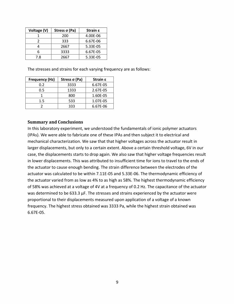
6. Calculate the strain ε and the stress σ of the actuator.

According to the NE 491 Lab 5 manual, the stress σ can be calculated from the applied force like

so: 2

6

bh

FL where σ is the stress tensor. The force applied can be calculated from the

cantilever equation EI

FL

3

3

and the moment of intertia I can be calculated using 12

3bhI

,

where b is the width and h is the thickness of the IPA actuator. The moment of intertia is

calculated to be 1.33E-15 m4. Assuming linear elasticity, we can calculate strain ε using Hooke’s

law: σ = Eε. The stresses and strains for each applied voltage are summarized in the table

below:

Frequency (Hz) Eff,em (%)

0.2 40%

0.5 16%

1 12%

1.5 8%

2 4%

9

Voltage (V) Stress σ (Pa) Strain ε

1 200 4.00E-06

2 333 6.67E-06

4 2667 5.33E-05

6 3333 6.67E-05

7.8 2667 5.33E-05

The stresses and strains for each varying frequency are as follows:

Frequency (Hz) Stress σ (Pa) Strain ε

0.2 3333 6.67E-05

0.5 1333 2.67E-05

1 800 1.60E-05

1.5 533 1.07E-05

2 333 6.67E-06

Summary and Conclusions

In this laboratory experiment, we understood the fundamentals of ionic polymer actuators

(IPAs). We were able to fabricate one of these IPAs and then subject it to electrical and

mechanical characterization. We saw that that higher voltages across the actuator result in

larger displacements, but only to a certain extent. Above a certain threshold voltage, 6V in our

case, the displacements starts to drop again. We also saw that higher voltage frequencies result

in lower displacements. This was attributed to insufficient time for ions to travel to the ends of

the actuator to cause enough bending. The strain difference between the electrodes of the

actuator was calculated to be within 7.11E-05 and 5.33E-06. The thermodynamic efficiency of

the actuator varied from as low as 4% to as high as 58%. The highest thermodynamic efficiency

of 58% was achieved at a voltage of 4V at a frequency of 0.2 Hz. The capacitance of the actuator

was determined to be 633.3 μF. The stresses and strains experienced by the actuator were

proportional to their displacements measured upon application of a voltage of a known

frequency. The highest stress obtained was 3333 Pa, while the highest strain obtained was

6.67E-05.

10

Lab 6 Polypyrrole Nanoparticles for pH Sensor


The objective of this laboratory is to build a pH meter by synthesis of a conducting polypyrrole

(Ppy) polymer film of varied thickness via electropolymerization. We then show how the open

circuit voltage of a film deposited using cyclic voltammetry (CV) varies linearly with the pH of

the solution. Using this technique, we can therefore measure the pH of a solution by measuring

the film’s open circuit potential once the sensor has been calibrated to determine linearity

characteristics.

The second objective of this laboratory is to calculate the polypyrrole’s film thickness accurately

using Faraday’s law and show how thicker films are less sensitive to changes in pH compared to

thin films.



Laboratory 6 part of the Nanotechnology Engineering Program 4B Lab Manuals, 2010. The only

deviation from procedure was that instead of using 5 cycles for the first cyclic voltammetry (CV)

part, we used 10 cycles.


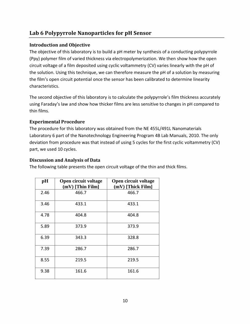
The following table presents the open circuit voltage of the thin and thick films.

pH Open circuit voltage

(mV) [Thin Film]

Open circuit voltage

(mV) [Thick Film]

2.46 466.7 466.7

3.46 433.1 433.1

4.78 404.8 404.8

5.89 373.9 373.9

6.39 343.3 328.8

7.39 286.7 286.7

8.55 219.5 219.5

9.38 161.6 161.6

11

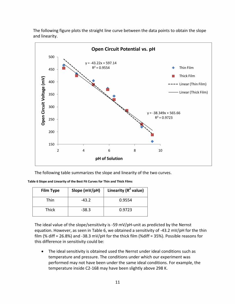
The following figure plots the straight line curve between the data points to obtain the slope and linearity.

The following table summarizes the slope and linearity of the two curves.

Table 6 Slope and Linearity of the Best Fit Curves for Thin and Thick Films

Film Type Slope (mV/pH) Linearity (R2 value)

Thin -43.2 0.9554

Thick -38.3 0.9723

The ideal value of the slope/sensitivity is -59 mV/pH-unit as predicted by the Nernst equation. However, as seen in Table 6, we obtained a sensitivity of -43.2 mV/pH for the thin film (% diff = 26.8%) and -38.3 mV/pH for the thick film (%diff = 35%). Possible reasons for this difference in sensitivity could be:

The ideal sensitivity is obtained used the Nernst under ideal conditions such as temperature and pressure. The conditions under which our experiment was performed may not have been under the same ideal conditions. For example, the temperature inside C2-168 may have been slightly above 298 K.

y = -43.22x + 597.14R² = 0.9554

y = -38.349x + 565.66R² = 0.9723

150

200

250

300

350

400

450

500

2 4 6 8 10

Op

en C

ircu

it V

olt

age

(mV

)

pH of Solution

Open Circuit Potential vs. pH

Thin Film

Thick Film

Linear (Thin Film)

Linear (Thick Film)

12

We assumed assuming 100% current efficiency for polypyrrole formation while calculating the ideal sensitivity. This efficiency, of course, is impossible to obtain in a real-life laboratory experiment.

The glass electrode in use is very sensitive and very variable. It could have been damaged ever so slightly causing it to have different absorbancies. The glass electrode could have also been dirty and contaminated leading to uneven film development.

The pH of the different buffer solutions provided to us may not have been exact.

The potentiostat provided to us is an electronic hardware equipment, and as with any hardware equipment has manufacturing errors, defects and differences. Hence, calibration against the ideal sensitivity value is necessary in a commercial pH electrode.

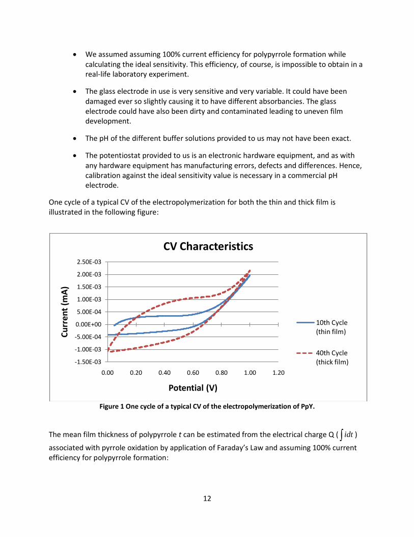
One cycle of a typical CV of the electropolymerization for both the thin and thick film is illustrated in the following figure:

Figure 1 One cycle of a typical CV of the electropolymerization of PpY.

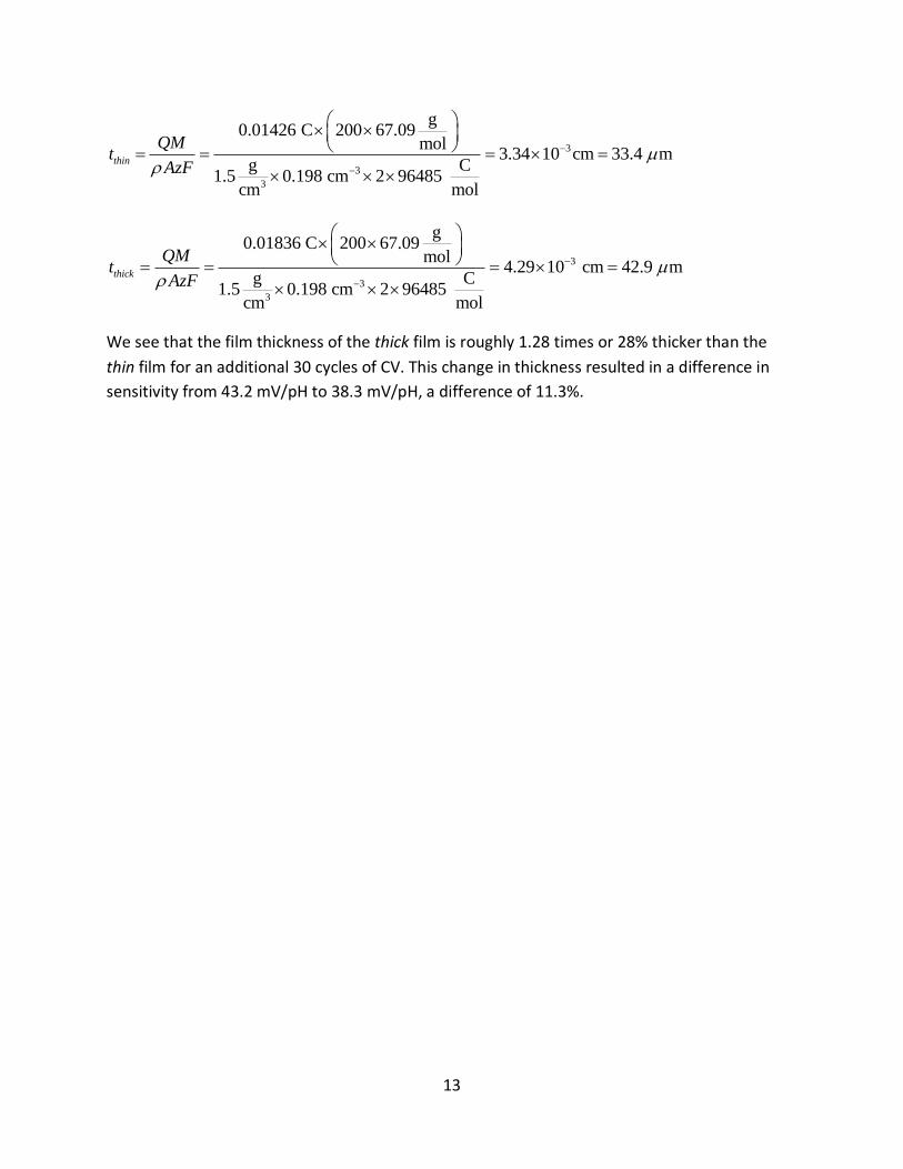
The mean film thickness of polypyrrole t can be estimated from the electrical charge Q ( idt )

associated with pyrrole oxidation by application of Faraday’s Law and assuming 100% current efficiency for polypyrrole formation:

-1.50E-03

-1.00E-03

-5.00E-04

0.00E+00

5.00E-04

1.00E-03

1.50E-03

2.00E-03

2.50E-03

0.00 0.20 0.40 0.60 0.80 1.00 1.20

Cu

rre

nt

(mA

)

Potential (V)

CV Characteristics

10th Cycle (thin film)

40th Cycle (thick film)

13

3

3

3

g0.01426 C 200 67.09

mol3.34 10 cm 33.4 m

g C1.5 0.198 cm 2 96485

cm mol

thin

QMt

AzF

3

3

3

g0.01836 C 200 67.09

mol4.29 10 cm 42.9 m

g C1.5 0.198 cm 2 96485

cm mol

thick

QMt

AzF

We see that the film thickness of the thick film is roughly 1.28 times or 28% thicker than the

thin film for an additional 30 cycles of CV. This change in thickness resulted in a difference in

sensitivity from 43.2 mV/pH to 38.3 mV/pH, a difference of 11.3%.

NE 455L/491 Nanomaterials Lab Report - Rajesh...

Documents

Transcript of NE 455L/491 Nanomaterials Lab Report - Rajesh...