Multifractal analysis of Bernoulli convolutionsassociated with Salem numbers

De-Jun Feng

The Chinese University of Hong Kong

Fractals and Related Fields II,Porquerolles - France, June 13th-17th 2011

Bernoulli convolutions

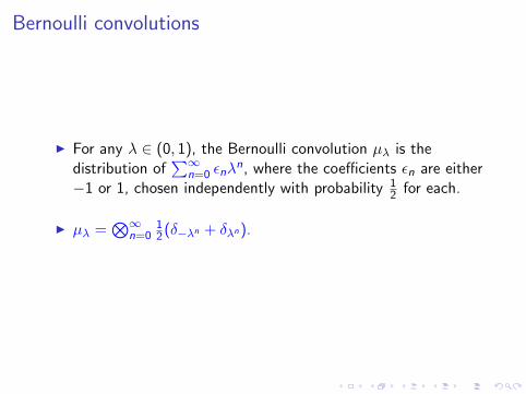
I For any λ ∈ (0, 1), the Bernoulli convolution µλ is thedistribution of

∑∞n=0 εnλ

n, where the coefficients εn are either−1 or 1, chosen independently with probability 1

2 for each.

I µλ =⊗∞

n=012(δ−λn + δλn).

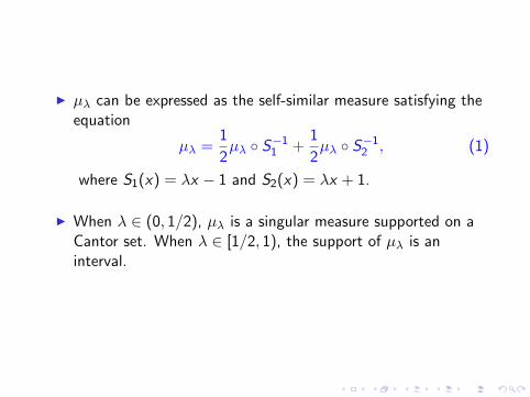
I µλ can be expressed as the self-similar measure satisfying theequation

µλ =1

2µλ ◦ S−1

1 +1

2µλ ◦ S−1

2 , (1)

where S1(x) = λx − 1 and S2(x) = λx + 1.

I When λ ∈ (0, 1/2), µλ is a singular measure supported on aCantor set. When λ ∈ [1/2, 1), the support of µλ is aninterval.

An Erdos problem

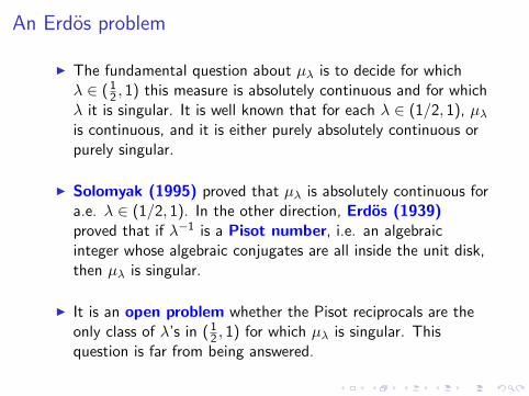
I The fundamental question about µλ is to decide for whichλ ∈ (1

2 , 1) this measure is absolutely continuous and for whichλ it is singular. It is well known that for each λ ∈ (1/2, 1), µλis continuous, and it is either purely absolutely continuous orpurely singular.

I Solomyak (1995) proved that µλ is absolutely continuous fora.e. λ ∈ (1/2, 1). In the other direction, Erdos (1939)proved that if λ−1 is a Pisot number, i.e. an algebraicinteger whose algebraic conjugates are all inside the unit disk,then µλ is singular.

I It is an open problem whether the Pisot reciprocals are theonly class of λ’s in (1

2 , 1) for which µλ is singular. Thisquestion is far from being answered.

Possible candidates for counter-examples

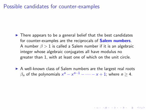
I There appears to be a general belief that the best candidatesfor counter-examples are the reciprocals of Salem numbers.A number β > 1 is called a Salem number if it is an algebraicinteger whose algebraic conjugates all have modulus nogreater than 1, with at least one of which on the unit circle.

I A well-known class of Salem numbers are the largest real rootsβn of the polynomials xn − xn−1 − · · · − x + 1; where n ≥ 4.

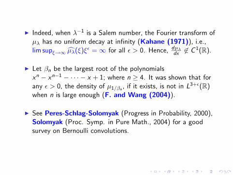
I Indeed, when λ−1 is a Salem number, the Fourier transform ofµλ has no uniform decay at infinity (Kahane (1971)), i.e.,lim supξ→∞ µλ(ξ)ξε =∞ for all ε > 0. Hence, dµλ

dx 6∈ C 1(R).

I Let βn be the largest root of the polynomialsxn − xn−1 − · · · − x + 1; where n ≥ 4. It was shown that forany ε > 0, the density of µ1/βn

, if it exists, is not in L3+ε(R)when n is large enough (F. and Wang (2004)).

I See Peres-Schlag-Solomyak (Progress in Probability, 2000),Solomyak (Proc. Symp. in Pure Math., 2004) for a goodsurvey on Bernoulli convolutions.

Our target

To study the local dimensions and the multifractal structure ofµλ when λ−1 is a Salem number in (1, 2). Very little has beenknown in the literature.

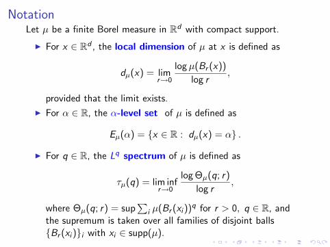
NotationLet µ be a finite Borel measure in Rd with compact support.

I For x ∈ Rd , the local dimension of µ at x is defined as

dµ(x) = limr→0

logµ(Br (x))

log r,

provided that the limit exists.

I For α ∈ R, the α-level set of µ is defined as

Eµ(α) = {x ∈ R : dµ(x) = α} .

I For q ∈ R, the Lq spectrum of µ is defined as

τµ(q) = lim infr→0

log Θµ(q; r)

log r,

where Θµ(q; r) = sup∑

i µ(Br (xi ))q for r > 0, q ∈ R, andthe supremum is taken over all families of disjoint balls{Br (xi )}i with xi ∈ supp(µ).

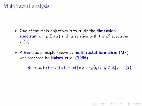
Multifractal analysis

I One of the main objectives is to study the dimensionspectrum dimH Eµ(α) and its relation with the Lq spectrumτµ(q)

I A heuristic principle known as multifractal formalism (MF)was proposed by Halsey et al (1986):

dimH Eµ(α) = τ∗µ(α) := inf{αq − τµ(q) : q ∈ R}. (2)

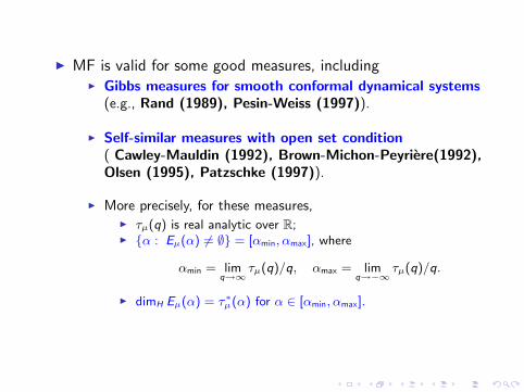
I MF is valid for some good measures, includingI Gibbs measures for smooth conformal dynamical systems

(e.g., Rand (1989), Pesin-Weiss (1997)).

I Self-similar measures with open set condition( Cawley-Mauldin (1992), Brown-Michon-Peyriere(1992),Olsen (1995), Patzschke (1997)).

I More precisely, for these measures,I τµ(q) is real analytic over R;I {α : Eµ(α) 6= ∅} = [αmin, αmax], where

αmin = limq→∞

τµ(q)/q, αmax = limq→−∞

τµ(q)/q.

I dimH Eµ(α) = τ∗µ(α) for α ∈ [αmin, αmax].

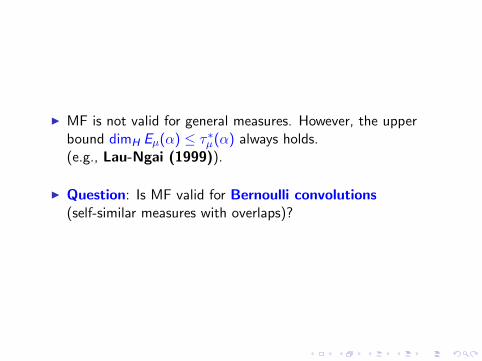
I MF is not valid for general measures. However, the upperbound dimH Eµ(α) ≤ τ∗µ(α) always holds.(e.g., Lau-Ngai (1999)).

I Question: Is MF valid for Bernoulli convolutions(self-similar measures with overlaps)?

I Question: Is MF valid for Bernoulli convolutions(self-similar measures with overlaps)?

I Difficulty:I hard to analyze the local behavior of µ and estimate the local

dimension of µ;

I hard to estimate the Lq-spectrum τµ(q) and its regularityproperty.

Historic remarks: When 1/λ is a Pisot number

I Many works in the literature: e.g., Alexander-Yorke (1984),Przytycki-Urbanski (1989), Alexander-Zagier (1991), Lau(1992), Ledrappier-Porzio (1994, 1996),Strichartz-Taylor-Zhang (1995), Lau-Ngai (1998, 1999),Lalley (1998), Porzio (1998), Vershik-Sidorov (1998), F.(2003, 2005, 2009), F. & Olivier (2003), F. & Lau (2009).

I Phase transition for q < 0 in the golden ratio case (

λ =√

5−12 ). That is, τµ(q) is not differentiable at some q < 0.

( F., 1999, 2005).

Similar exceptional phenomena for other self-similar measureswith overlaps (e.g., Hu-Lau (2001), F. -Lau-Wang (2005),Shmerkin (2005), Testud (2006))

I So far the most complete result is the following (F., 2009):

I dimH Eµ(α) = τ∗µ(α) for α ∈ [τ ′µ(∞), τ ′µ(0−)].

I ∃ an interval I ⊂ supp(µ) so that, for ν = µ|I ,I Eν(α) 6= ∅ if and only if α ∈ [τ ′ν(+∞), τ ′ν(−∞)].

I dimH Eν(α) = τ∗ν (α) for each α ∈ [τ ′ν(+∞), τ ′ν(−∞)].

I τν(q) = τµ(q) for q ≥ 0.

I The above results hold for self-similar measures with weakseparation condition (F. & Lau (2009)); this condition wasintroduced by Lau-Ngai (1999).

I We point out that in the pisot case, τµ is differentiable on(0,∞) (F. (2003)); and [τ ′µ(∞), τ ′µ(0−)] contains aneighborhood of 1. (F. & Sidorov (2011)).

I Based on products of random matrices and thethermodynamic formalism.

Historic remarks: Non-Pisot case

I For every λ ∈ (1/2, 1),

Eµλ(α) 6= ∅ and dimH Eµλ(α) = τ∗µλ

(α)

for those α = τ ′µλ(q), q > 1, provided that τ ′µλ

(q) exists at q.The result holds for all self-conformal measures withoverlaps. (F., 2007)

I Key idea: Show that for any q > 1, ∃ a measure νq such that

νq(Br (x)) � r−τµ(q)µλ(B16r (x))q.

(Inspired from works of Peres-Solomyak (2000), andBrown-Michon-Peyriere (1992)) .Then apply some large-deviation like arguments as inBrown-Michon-Peyriere (1992), Ben Nasr (1994) and Testud(2006).

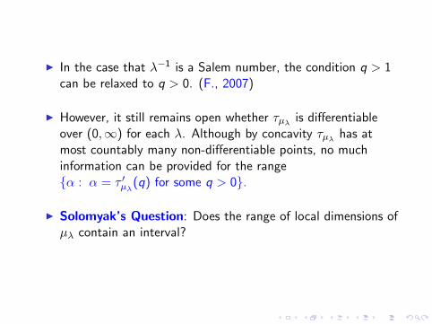
I In the case that λ−1 is a Salem number, the condition q > 1can be relaxed to q > 0. (F., 2007)

I However, it still remains open whether τµλis differentiable

over (0,∞) for each λ. Although by concavity τµλhas at

most countably many non-differentiable points, no muchinformation can be provided for the range{α : α = τ ′µλ

(q) for some q > 0}.

I Solomyak’s Question: Does the range of local dimensions ofµλ contain an interval?

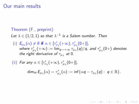
Our main results

Theorem (F., preprint)

Let λ ∈ (1/2, 1) so that λ−1 is a Salem number. Then

(i) Eµλ(α) 6= ∅ if α ∈ [τ ′νλ

(+∞), τ ′µλ(0+)],

where τ ′µλ(+∞) := limq→+∞ τµλ

(q)/q, and τ ′µλ(0+) denotes

the right derivative of τµλat 0.

(ii) For any α ∈ [τ ′νλ(+∞), τ ′µλ

(0+)],

dimH Eµλ(α) = τ∗µλ

(α) := inf{αq − τµλ(q) : q ∈ R}.

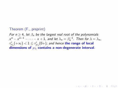
Theorem (F., preprint)

For n ≥ 4, let βn be the largest real root of the polynomialsxn − xn−1 − · · · − x + 1, and let λn = β−1

n . Then for λ = λn,τ ′νλ

(+∞) < 1 ≤ τ ′µλ(0+); and hence the range of local

dimensions of µλ contains a non-degenerate interval.

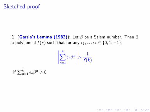
Sketched proof

1. (Garsia’s Lemma (1962)): Let β be a Salem number. Then ∃a polynomial f (x) such that for any ε1, . . . εk ∈ {0, 1,−1},∣∣∣∣∣

k∑n=1

εnβn

∣∣∣∣∣ > 1

f (k)

if∑k

n=1 εnβn 6= 0.

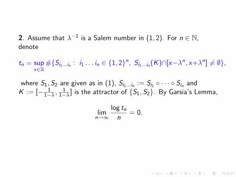
2. Assume that λ−1 is a Salem number in (1, 2). For n ∈ N,denote

tn = supx∈R

#{Si1...in : i1 . . . in ∈ {1, 2}n, Si1...in(K )∩[x−λn, x+λn] 6= ∅},

where S1, S2 are given as in (1), Si1...in := Si1 ◦ · · · ◦ Sin andK := [− 1

1−λ ,1

1−λ ] is the attractor of {S1,S2}. By Garsia’s Lemma,

limn→∞

log tnn

= 0.

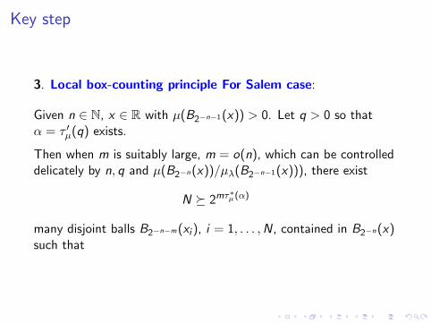
Key step

3. Local box-counting principle For Salem case:

Given n ∈ N, x ∈ R with µ(B2−n−1(x)) > 0. Let q > 0 so thatα = τ ′µ(q) exists.

Then when m is suitably large, m = o(n), which can be controlleddelicately by n, q and µ(B2−n(x))/µλ(B2−n−1(x))), there exist

N � 2mτ∗µ(α)

many disjoint balls B2−n−m(xi ), i = 1, . . . ,N, contained in B2−n(x)such that

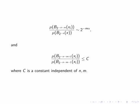
µ(B2−n−m(xi ))

µ(B2−n(x))∼ 2−mα,

and

µ(B2−n−m+1(xi ))

µ(B2−n−m−1(xi ))≤ C

where C is a constant independent of n,m.

Comparison

Classical box-counting principle

For any measure µ, let q > 0 so that α = τ ′µ(q) exists and letk ∈ N. Then there exists a sequence rn ↓ 0 such that for each n,

there are Nn � r−τ∗µ(α)n many disjoint balls Brn(xi ), so that

µ(Brn(xi )) ∼ rαn ,

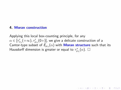
4. Moran construction

Applying this local box-counting principle, for anyα ∈ [τ ′νλ

(+∞), τ ′µλ(0+)], we give a delicate construction of a

Cantor-type subset of Eµλ(α) with Moran structure such that its

Hausdorff dimension is greater or equal to τ∗µλ(α). �

Question: Since Bernoulli convolution associated with Salemnumbers may have a rich multifractal structure, can we concludethat they are singular?

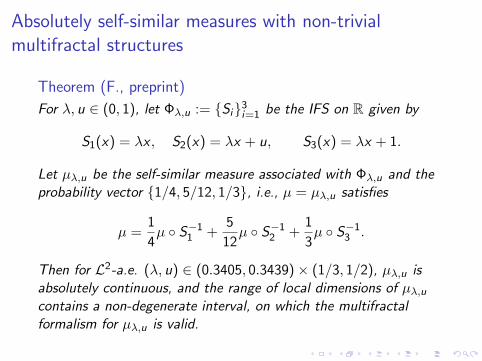
Absolutely self-similar measures with non-trivialmultifractal structures

Theorem (F., preprint)

For λ, u ∈ (0, 1), let Φλ,u := {Si}3i=1 be the IFS on R given by

S1(x) = λx , S2(x) = λx + u, S3(x) = λx + 1.

Let µλ,u be the self-similar measure associated with Φλ,u and theprobability vector {1/4, 5/12, 1/3}, i.e., µ = µλ,u satisfies

µ =1

4µ ◦ S−1

1 +5

12µ ◦ S−1

2 +1

3µ ◦ S−1

3 .

Then for L2-a.e. (λ, u) ∈ (0.3405, 0.3439)× (1/3, 1/2), µλ,u isabsolutely continuous, and the range of local dimensions of µλ,ucontains a non-degenerate interval, on which the multifractalformalism for µλ,u is valid.

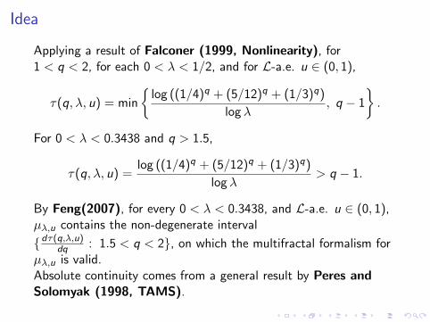
Idea

Applying a result of Falconer (1999, Nonlinearity), for1 < q < 2, for each 0 < λ < 1/2, and for L-a.e. u ∈ (0, 1),

τ(q, λ, u) = min

{log ((1/4)q + (5/12)q + (1/3)q)

log λ, q − 1

}.

For 0 < λ < 0.3438 and q > 1.5,

τ(q, λ, u) =log ((1/4)q + (5/12)q + (1/3)q)

log λ> q − 1.

By Feng(2007), for every 0 < λ < 0.3438, and L-a.e. u ∈ (0, 1),µλ,u contains the non-degenerate interval

{dτ(q,λ,u)dq : 1.5 < q < 2}, on which the multifractal formalism for

µλ,u is valid.Absolute continuity comes from a general result by Peres andSolomyak (1998, TAMS).

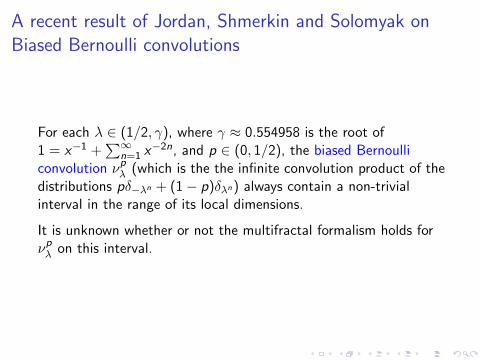
A recent result of Jordan, Shmerkin and Solomyak onBiased Bernoulli convolutions

For each λ ∈ (1/2, γ), where γ ≈ 0.554958 is the root of1 = x−1 +

∑∞n=1 x−2n, and p ∈ (0, 1/2), the biased Bernoulli

convolution νpλ (which is the the infinite convolution product of the

distributions pδ−λn + (1− p)δλn) always contain a non-trivialinterval in the range of its local dimensions.

It is unknown whether or not the multifractal formalism holds forνpλ on this interval.

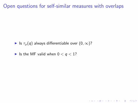
Open questions for self-similar measures with overlaps

I Is τµ(q) always differentiable over (0,∞)?

I Is the MF valid when 0 < q < 1?

D. J. Feng, Multifractal analysis of Bernoulli convolutionsassociated with Salem numbers. Preprint. (available onwww.math.cuhk.edu.hk/∼ djfeng)

Thank you!!!