M

Ob

ject

arm

Image sensor

plane

Micro-polarizer

array

Light

1 pixel

Polarizer

Ultrafast

Reference arm

object

Quarter-

wave plate

Polarization-

imaging camera

Femtosecondpulsed laser

Plate 1 (Figure 1.13) Schematic diagram of parallel phase-shifting digital holography system using afemtosecond pulsed laser

(a) (b) 2π

0

Plate 2 (Figure 1.15) Reconstructed images. (a) By parallel phase-shifting digital holography,(b) by a diffraction integral alone

Multi-dimensional Imaging, First Edition. Edited by Bahram Javidi, Enrique Tajahuerce and Pedro Andrés.© 2014 John Wiley & Sons, Ltd. Published 2014 by John Wiley & Sons, Ltd.

(a) (b)

Plate 3 (Figure 2.9) (a) Spherical lens configuration. Mannequin image with irradiated area in red;mannequin hologram amplitude reconstruction. (b) Cylindrical lens configuration. Mannequin imagewith irradiated area in red; mannequin hologram amplitude reconstruction

Plate 4 (Figure 2.10) (From left to right) Mannequin image with irradiated area in red; mannequinhologram amplitude reconstruction at different scanning time and superposition of the most significantframes

0.5

2.2

0.6

0.8

1.2

1.4

1.6

1.8

1

1.8

1.6

1.4

1.2

2

1

(a)

‒0.5

‒0.5

0.5

1

0

‒1‒1

0.5 1

(b)

‒0.5‒1

y

‒0.5

0.5

1

0

‒1

y

0x

0x

Plate 5 (Figure 3.10) Single point resolution in a transversal plane (from Fournier et al. 2010):(a) x-resolution map normalized by the value of x-resolution on the optical axis; (b) normalizedz-resolution map. The squares in the center of figures (a) and (b) represent the sensor boundaries. Source:Fournier C., Denis L., and Fournel T., 2010. Reproduced with permission from the Optical Society

0 0.1 0.2 0.3 0.4 0.5 0.6 0.7 0.8 0.9 10

10

20

30

40

50

60

z/z0

M/S

db1 (Haar) waveletSym2 waveletCoif1 waveletUnit Operator

Plate 6 (Figure 4.6) Simulation results showing the normalized compressive sampling ratio for dif-ferent sparsifying bases [26]. Source: Y. Rivenson, A. Stern, and B. Javidi 2013. Reproduced withpermission from The Optical Society

(b) (c)(a)

(e) (f)(d)

Plate 7 (Figure 4.9) Reconstruction examples of the B (forward) and U (backward) planes. (a) Recon-struction of the B plane form 100% of the projections. (b) CS reconstruction of the B plane forms 6% ofthe projections. (c) CS reconstruction of the B plane forms 2.5% of the projections. (d) Reconstructionof the U plane forms 100% of the projections. (e) CS reconstruction of the U plane forms 6% of theprojections. (f) CS reconstruction of the U plane forms 2.5% of the projections

10.5

0–0.5–1

1.281.26

x (mm)

σt = 50 fs

t (ps)

10.5

0–0.5–1

t (ps)

1.24

1.281.26

x (mm)

1.24

Plate 8 (Figure 5.6) Spatiotemporal profiles of the fifth diffraction order of a 100 lines/inch diffractivegrating for an input pulse width of 𝜎t = 50 fs. The right part of the figure is obtained after focusing withan achromatic lens doublet and the left part by focusing with the DOE-based system. Note that the timeorigin is chosen arbitrarily. Source: Mínguez-Vega, G., Tajahuerce, E., Fernández-Alonso, M., Climent,V., Lancis, J., Caraquitena, J., Andrés, P., (2007). Figure 6. Reproduced with permission from The OpticalSociety

–200–300

–100 0

0

Tim

e (

fs)

100

300

–300

0

300

–300

0

300

–400

0

400

–400

0

400

–300

0

Tim

e (

fs) 300

–300

0

Tim

e (

fs)

300

–300

0

Tim

e (

fs) 300

200

–200 –100 0 100 200 –200 –100 0 100 200

–200 –100 0 100 200

–300 –200 –100 0 100 300200

–300 –200 –100 0

0 0.1 0.2 0.3 0.4 0.5 0.6 0.7 0.8 0.9 1

Lateral coordinate x (μm) Lateral coordinate x (μm)

100 300200 –300 –200 –100 0 100 300200

–300 –200 –100 0 100 300200

Plate 9 (Figure 5.9) Normalized spatiotemporal light intensity after low NA focusing of the beamletscoming from a diffractive grating (0th, +1st, +2nd, and +3rd diffraction orders from top to bottom) with(left column) and without (right column) DCM. Measurements were captured using STARFISH [18]. Themaximum frequency component, for the third diffraction order, is 35.4 lp/mm. Source: Martínez-Cuenca,R., Mendoza-Yero, O., Alonso, B., Sola, Í. J., Mínguez-Vega, G., Lancis, J. (2012). Figure 2. Reproducedwith permission from The Optical Society

(a) (b) (c)

Plate 10 (Figure 6.6) (a) Out of focus color intensity of the alga Odontella sp., (b) refocused intensity,(c) composite phase image of the RGB channels

45

35

25

Ave

rag

e C

on

tra

st

Ave

rag

e C

on

tra

st

15

20

10

520 40 60 80 100

Average Intensity

(a)

20 3010

10

20

30

40

50

40 50 60 8070

Average Intensity

(b)

120 140 160

40

30

Chlorella

Giardia

Scenedesmus

Chlorella

Giardia

Scenedesmus

Plate 11 (Figure 6.13) Feature space representation using (a) intensity information of the detectedparticles of the three species, and (b) compensated phase of detected particles of the three species

–10 0 10 20 30v

0.5

1.0

1.5

2.0I

1

0.75

0.5

0.25

0

Plate 12 (Figure 7.14) Imaging of two neighboring point-like phase defects using VDIC with differentparameters

Plate 13 (Figure 7.15) Combination of an image obtained using Zernike phase contrast (hue) and oneobtained using DIC (intensity) in order to visualize a phase structure

250

4.4 MW/cm2

5.6 MW/cm2

14.8 MW/cm2

200

150

z (n

m)

x (nm)

y (nm)

100

50

0

200

150

100

50

00

50100

150200

250

Plate 14 (Figure 8.7) Movement of a 200 nm polystyrene particle in the trapping volume at differentintensities: (blue) 4.4 MW/cm2, (black) 5.6 MW/cm2, and (red) 14.8 MW/cm2

12005.6 MW/cm2

16.3 MW/cm2

46.6 MW/cm2

1000

800

600

z (n

m)

400

200

0

200400

x (nm) y (nm)600 0200

400600

Plate 15 (Figure 8.10) Three-dimensional display of the gold nanoparticle movements

Cell culturein perfusionchamber

Objective

CCD

(a)

Refer

ence

O

0

Phase[Deg.]

Thickness[μm]

10 μm

(b)

0

2.9

5.8

8.7

11.6

20

40

60

80

100

120

140

160

Plate 16 (Figure 9.2) Digital holographic microscopy (DHM) of living mouse cortical neurons inculture. (a) Schematic representation of cultured cells mounted in a closed perfusion chamber andtrans-illuminated (b) 3D perspective image in false colors of a living neuron in culture. Each pixel repre-sents a quantitative measurement of the phase retardation or cellular optical path length (OPL) inducedby the cell with a sensitivity corresponding to a few tens of nanometers. By using the measured meanvalue of the neuronal cell body refractive index, resulting from the decoupling procedure, scales (right),which relate OPL (∘) to morphology in the z-axis (μm), can be constructed

Illumination beam

Input plane: Object + Pinhole

Lens

CCD

Chamber withsuspended

particles

F

F

Plate 17 (Figure 10.4) Digital holography super-resolution setup. Source: Zalevsky Z., Gur E.,Garcia J., Micó V., Javidi B. 2012. Figure 1. Reproduced with permission from The Optical Society

Δθ

(x3,θ3) (x2,θ2) (x2,θ2)(x1,θ1)

(a) (b)

(x0,θ0)

d g´t

g = f

Plate 18 (Figure 11.17) (a) Scheme for the calculation of the plenoptic function in planes parallel tothe MLA; (b) the plenoptic field as evaluated in the plane of the camera lens is equivalent to the onecaptured with an IP setup

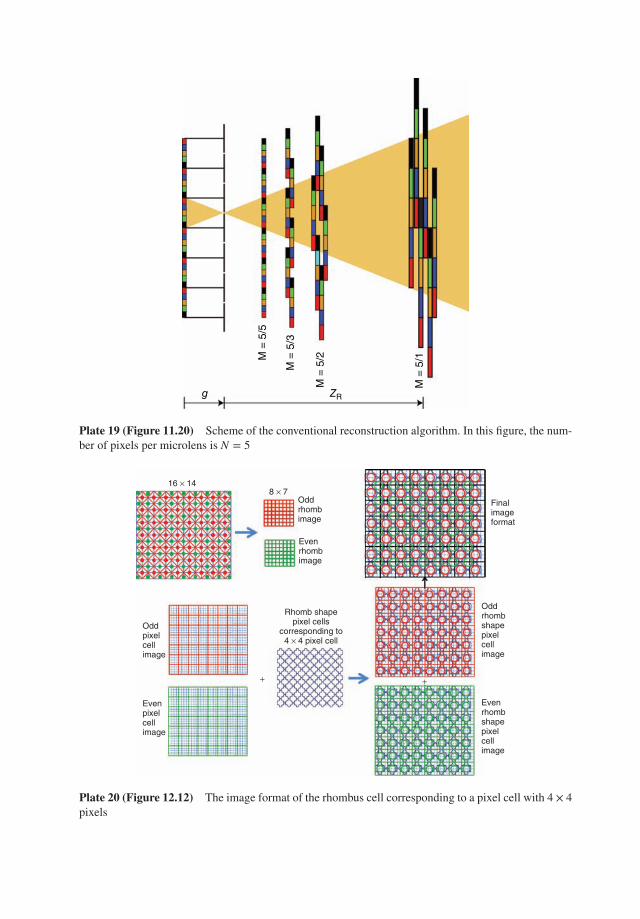
M =

5/5

M =

5/3

M =

5/2

ZRg

M =

5/1

Plate 19 (Figure 11.20) Scheme of the conventional reconstruction algorithm. In this figure, the num-ber of pixels per microlens is N = 5

Oddpixelcellimage

Rhomb shapepixel cells

corresponding to4 × 4 pixel cell

Evenpixelcellimage

Oddrhombshapepixelcellimage

Finalimageformat

Oddrhombimage

16 × 148 × 7

+ +

Evenrhombimage

Evenrhombshapepixelcellimage

Plate 20 (Figure 12.12) The image format of the rhombus cell corresponding to a pixel cell with 4 × 4pixels

Right

Image format

Bottom(K = + 4)

Top(K = − 4)

K = 0

Center Left

Plate 21 (Figure 12.16) Image format of a triangular pyramid

(b)

Plate 22 (Figure 13.8) Reconstruction of FP-HS. (b) Example of the reconstructed image fromfull-color FP-HS hologram [20]. Source: T. Utsugi and M. Yamaguchi 2013. Reproduced with permissionfrom The Optical Society

(a) (b) (c)

Plate 23 (Figure 13.23) Reconstructed images from the FP HS recorded from the captured light-fielddata. (a) Sushi, (b) vegetables, and (c) human face

(a) 1st IC (b) 2nd IC (c) 3rd IC

(e)

(d)

(f)

A

BC

D

E

2800 2900 3000 3100

Wavenumber [cm−1

]

SR

S s

pectr

um

[a.u

.]

Lipid (A) Cytoplasm (B) Filament (C) Nucleus(D) Water (E)

x1/4

2800 2900 3000 3100

Wavenumber [cm−1

]

1st 2nd 3rd

IC s

pectr

um

[a.u

.]

Plate 24 (Figure 15.12) Spectral imaging of a rat liver tissue [28]. 91 images at wavenumbers from2800–3100 cm−1 were taken and averaged over 10 times. The total acquisition time was <30 s. Thespectral images were analyzed by using 5 ICs. (a) First IC image reflecting the distribution of lipid-richregion. (b) Second IC image reflecting the distribution of water-rich regions. (c) Third IC image reflect-ing the distribution of protein-rich region. (d) IC spectra. (e) Multicolor image produced by combiningimages (a–c) and inverting the contrast. (a)–(e) are explained in the text. (f) SRS spectra in locationsindicated by arrows in (e). Scale bar: 20 μm. Source: Y. Ozeki, W. Umemura, Y. Otsuka, S. Satoh, H.Hashimoto, K. Sumimura, N. Nishizawa, K. Fukui, and K. Itoh 2012. Reproduced with permission fromNature Publishing

2800 2900 3000 3100

Wavenumber [cm−1]

1st 4th

IC s

pectr

um

[a.u

.]

(d) (e) (f)

(g) (h) (i)

(a) (b) (c)

Plate 25 (Figure 15.13) Sectioned spectral imaging of intestinal villi in the mouse [28]. 91 images atwavenumbers from 2800–3100 cm−1 were taken by changing the z position by 5.6 μm. The total acqui-sition time was 24 s. The spectral images were analyzed by using 4 ICs. The first IC (cytoplasm) and thefourth IC (nuclei) images were colored cyan and yellow, respectively, and then combined and the con-trast was inverted. (a–h). Sectioned multicolor images. (f). Spectra of the first and fourth ICs. Scale bar:20 μm. Source: Y. Ozeki, W. Umemura, Y. Otsuka, S. Satoh, H. Hashimoto, K. Sumimura, N. Nishizawa,K. Fukui, and K. Itoh 2012. Reproduced with permission from Nature Publishing

510 nm 520 nm 530 nm 540 nm

550 nm 560 nm 570 nm 620 nm

630 nm 640 nm 650 nm 660 nm

670 nm 680 nm 860 nm RGB

Plate 26 (Figure 16.5) Multispectral data cube reconstructed using CS. In the VIS band, the reflectancefor each spectral channel is represented by means of a 256 × 256 pseudo-color image. In the NIR bandwe show a gray-scale representation. A colorful image of the scene made up from the conventional RGBchannels is also included. Source: F. Soldevila, E. Irles, V. Durán, P. Clemente, M. Fernández-Alonso,E. Tajahuerce, and J. Lancis 2013, Figure 4. Reproduced with permission from Springer

RGB image

P

P

P90°

P45°

PP0°

P135°

Wavelength (nm)

490

Po

lari

zati

on

520 565 590 610 640 660 680

Plate 27 (Figure 16.8) Multispectral image cube reconstructed by CS algorithm for four differentconfigurations of the polarization analyzer. The RGB image of the object is also included. In the VISspectrum all channels are represented by pseudo-color images and a gray-scale representation is usedfor the wavelength closer to the NIR spectrum. Source: F. Soldevila, E. Irles, V. Durán, P. Clemente,M. Fernández-Alonso, E. Tajahuerce, and J. Lancis 2013, Figure 5. Reproduced with permission fromSpringer

S1

460 nm 480 nm 500 nm 520 nm 540 nm 560 nm 580 nm 720 nm1

0.8

0.6

0.4

0.2

0

−0.2

−0.4

−0.6

−0.8

−1

S2

S3

Plate 28 (Figure 16.11) Spatial distribution of the Stokes parameters of the polystyrene piece. Eachdistribution is represented by a pseudo-colored 128 × 128 pixels picture. The values range from−1 (blue)to 1 (red)

00.4 0.6 0.8 1 1.2 1.4

Wavelength (microns)

1.6 1.8 2 2.2 2.4

0.2

Tropical

Baseline

Desert

VIS NIR SWIR

MWIR LWIR

0.4

Tra

nsm

issi

on

0.6

0.8

1

03 4 5 6 7 8 9 10 11 12 13 14

Wavelength (microns)

0.2Tropical

Baseline

Desert

0.4Tra

nsm

issi

on

0.6

0.8

0.9

0.7

0.5

0.3

0.1

1

Plate 29 (Figure 17.11) Ground to space atmospheric transmission windows

30

100

200

300

400

500

600

700

4 5 6 7 8

Wavelength (microns)

Desert

230 K

280 K

Baseline

Tropical

Path

Radia

nce (

uW

/cm

2um

ar)

9 10 11 12 13 14

Plate 30 (Figure 17.15) Examples of path emission along a ground to space line of sight as a functionof range and atmospheric conditions