This article was downloaded by: [Tulane University]On: 21 September 2013, At: 04:46Publisher: Taylor & FrancisInforma Ltd Registered in England and Wales Registered Number: 1072954 Registeredoffice: Mortimer House, 37-41 Mortimer Street, London W1T 3JH, UK

International Journal of RemoteSensingPublication details, including instructions for authors andsubscription information:http://www.tandfonline.com/loi/tres20

Model of electronic-vibrational kineticsof the O3 and O2 photolysis products inthe middle atmosphere: applicationsto water vapour retrievals from SABER/TIMED 6.3 µm radiance measurementsValentine Yankovsky a , Rada Manuilova a , Alexander Babaev a ,Artem Feofilov b c & Alexander Kutepov b ca Institute of Physics, St. Petersburg State University, 198504,Russiab The Catholic University of America, 620 Michigan Avenue,Washington, DC, 20064, USAc NASA Goddard Space Flight Center, Mailcode 674, GreenbeltRoad, Greenbelt, MD, 20771, USAPublished online: 24 Jun 2011.

To cite this article: Valentine Yankovsky , Rada Manuilova , Alexander Babaev , Artem Feofilov& Alexander Kutepov (2011) Model of electronic-vibrational kinetics of the O3 and O2 photolysisproducts in the middle atmosphere: applications to water vapour retrievals from SABER/TIMED6.3 µm radiance measurements, International Journal of Remote Sensing, 32:11, 3065-3078, DOI:10.1080/01431161.2010.541506

To link to this article: http://dx.doi.org/10.1080/01431161.2010.541506

PLEASE SCROLL DOWN FOR ARTICLE

Taylor & Francis makes every effort to ensure the accuracy of all the information (the“Content”) contained in the publications on our platform. However, Taylor & Francis,our agents, and our licensors make no representations or warranties whatsoever as tothe accuracy, completeness, or suitability for any purpose of the Content. Any opinionsand views expressed in this publication are the opinions and views of the authors,and are not the views of or endorsed by Taylor & Francis. The accuracy of the Contentshould not be relied upon and should be independently verified with primary sourcesof information. Taylor and Francis shall not be liable for any losses, actions, claims,proceedings, demands, costs, expenses, damages, and other liabilities whatsoever or

howsoever caused arising directly or indirectly in connection with, in relation to or arisingout of the use of the Content.

This article may be used for research, teaching, and private study purposes. Anysubstantial or systematic reproduction, redistribution, reselling, loan, sub-licensing,systematic supply, or distribution in any form to anyone is expressly forbidden. Terms &Conditions of access and use can be found at http://www.tandfonline.com/page/terms-and-conditions

Dow

nloa

ded

by [

Tul

ane

Uni

vers

ity]

at 0

4:46

21

Sept

embe

r 20

13

International Journal of Remote SensingVol. 32, No. 11, 10 June 2011, 3065–3078

Model of electronic-vibrational kinetics of the O3 and O2 photolysisproducts in the middle atmosphere: applications to water vapourretrievals from SABER/TIMED 6.3 µm radiance measurements

VALENTINE YANKOVSKY*†, RADA MANUILOVA†, ALEXANDERBABAEV†, ARTEM FEOFILOV‡§ and ALEXANDER KUTEPOV‡§

†Institute of Physics, St. Petersburg State University, 198504, Russia‡The Catholic University of America, 620 Michigan Avenue, Washington DC 20064, USA§NASA Goddard Space Flight Center, Mailcode 674, Greenbelt Road, Greenbelt, MD

20771, USA

In this work, we present a methodology of simple yet accurate calculations ofH2O(v2) vibrational levels pumping from the collisions with vibrationally excitedO2(X3�−

g, v = 1) molecules, which is required for correct retrievals of H2O volumemixing ratios from the 6.3 µm band radiance. The electronic-vibrational kineticsmodel of O2 and O3 photolysis products used in this study includes 44 electron-ic-vibrational states of the O2 molecule (three states of O2(b1�+

g, v), six statesof O2(a1�g, v) and 35 states of O2(X3�−

g, v)) as well as the first excited state ofatomic oxygen, O(1D) and considers more than 100 photochemical reactions link-ing these states. We introduce the Resulting Quantum Output (RQO) approachthat describes the O2(X3�−

g, v = 1) production quantum yield per one act ofO3 photolysis in the Hartley, Huggins, Chappuis and Wulf bands (200–900 nm).We demonstrate that the RQO weakly depends on latitude and season, and sug-gest a parameterization formula for the altitude dependence of this parameter. Weshow the application of RQO to H2O retrievals from the 6.3 m broadband radi-ance measured by the Sounding of the Atmosphere using Broadband EmissionRadiometry (SABER)/Thermosphere Ionosphere Mesosphere Energetics andDynamics (TIMED) instrument that has been performing remote sensing of theEarth’s atmosphere in the 13–110 km altitude range from 2002 onwards.

1. Introduction

This paper describes an important component required for the correct interpretationof 6.3 µm water vapour radiance in the mesosphere and lower thermosphere (MLT),the region that remains the least explored part of the Earth’s atmosphere. This areais sensitive both to external influences from the Sun and to radiative transfer fromthe lower atmosphere, and is therefore considered to be an ‘early warning system’for global changes in atmosphere. Water vapour is one of the key components of themiddle atmosphere that influences the composition and energy budget of this region(Brasseur and Solomon 2005, Sonnemann et al. 2005). An adequate interpretationof H2O infrared measurements requires an exact knowledge of all processes popu-lating and depopulating the H2O(ν2) vibrational states. Among these processes, the

*Corresponding author. Email: vyankovsky@gmail.com

International Journal of Remote SensingISSN 0143-1161 print/ISSN 1366-5901 online © 2011 Taylor & Francis

http://www.tandf.co.uk/journalsDOI: 10.1080/01431161.2010.541506

Dow

nloa

ded

by [

Tul

ane

Uni

vers

ity]

at 0

4:46

21

Sept

embe

r 20

13

3066 V. Yankovsky et al.

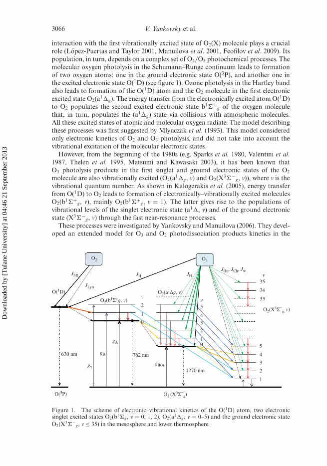
interaction with the first vibrationally excited state of O2(X) molecule plays a crucialrole (Lopez-Puertas and Taylor 2001, Manuilova et al. 2001, Feofilov et al. 2009). Itspopulation, in turn, depends on a complex set of O2/O3 photochemical processes. Themolecular oxygen photolysis in the Schumann–Runge continuum leads to formationof two oxygen atoms: one in the ground electronic state O(3P), and another one inthe excited electronic state O(1D) (see figure 1). Ozone photolysis in the Hartley bandalso leads to formation of the O(1D) atom and the O2 molecule in the first electronicexcited state O2(a1�g). The energy transfer from the electronically excited atom O(1D)to O2 populates the second excited electronic state b1�+

g of the oxygen moleculethat, in turn, populates the (a1�g) state via collisions with atmospheric molecules.All these excited states of atomic and molecular oxygen radiate. The model describingthese processes was first suggested by Mlynczak et al. (1993). This model consideredonly electronic kinetics of O2 and O3 photolysis, and did not take into account thevibrational excitation of the molecular electronic states.

However, from the beginning of the 1980s (e.g. Sparks et al. 1980, Valentini et al.1987, Thelen et al. 1995, Matsumi and Kawasaki 2003), it has been known thatO3 photolysis products in the first singlet and ground electronic states of the O2

molecule are also vibrationally excited (O2(a1�g, v) and O2(X3�−g, v)), where v is the

vibrational quantum number. As shown in Kalogerakis et al. (2005), energy transferfrom O(1D) to O2 leads to formation of electronically–vibrationally excited moleculesO2(b1�+

g, v), mainly O2(b1�+g, v = 1). The latter gives rise to the populations of

vibrational levels of the singlet electronic state (a1�, v) and of the ground electronicstate (X3�−

g, v) through the fast near-resonance processes.These processes were investigated by Yankovsky and Manuilova (2006). They devel-

oped an extended model for O3 and O2 photodissociation products kinetics in the

O2 O3

JHu, JCh, Jwv

35

34

33

5

v5

4

3

2

10

4

3

2

1

JH JH

v

2

1

0

762 nm

gIRA

1270 nm

630 nm

O(3P) O2 (X3Σ−

g)

O2(X3Σ−g, v)

gA

gB

gγ

JLyα

JSR

O(1D)

O2(b1Σ+g, v)

O2(a1Δg, v)

Figure 1. The scheme of electronic–vibrational kinetics of the O(1D) atom, two electronicsinglet excited states O2(b1�g, v = 0, 1, 2), O2(a1�g, v = 0–5) and the ground electronic stateO2(X3�−

g, v ≤ 35) in the mesosphere and lower thermosphere.

Dow

nloa

ded

by [

Tul

ane

Uni

vers

ity]

at 0

4:46

21

Sept

embe

r 20

13

Atmospheric studies by optical methods 3067

MLT, hereafter known as the YM-2006 model. In the present work, we use this modelfor the calculations of the O2(X3�−

g, v = 1–35) populations.In this work, we have focused our efforts on studying the O2(X3�−

g, v = 1) statepopulation behaviour with respect to various atmospheric conditions and on theparameterization of this source of H2O(010) population, which is required for oper-ational retrieval of H2O volume mixing ratio (VMR) retrieval from the 6.3 µmband emission measured, in particular, by the Sounding of the Atmosphere usingBroadband Emission Radiometry (SABER)/Thermosphere Ionosphere MesosphereEnergetics and Dynamics (TIMED) satellite limb infrared radiometer.

1.1 Remote sensing of the Earth’s atmosphere using the SABER instrument on boardthe TIMED satellite

The TIMED satellite was launched on 7 December 2001 into a 74.1◦ inclined 625 kmorbit with a period of 1.7 hours. The TIMED mission was focused on the energeticsand dynamics of the MLT region (60–180 km) (Yee et al. 1999). SABER, one of fourinstruments on TIMED, is a 10 channel broadband limb-scanning infrared radiome-ter covering the spectral range from 1.27 µm to 17 µm. SABER provides verticalprofiles of kinetic temperature, pressure, ozone, carbon dioxide, water vapour, atomicoxygen, atomic hydrogen and volume emission rates in the NO (5.3 µm) and OHMeinel and O2(a1�g) bands. The vertical instantaneous field of view of the instrumentis approximately 2.0 km at 60 km altitude, the vertical sampling interval is ∼0.4 km,and the atmosphere is scanned from below the surface up to 400 km tangent height.The instrument performs one vertical scan every 53 s, the scans are performed both inthe upwards and downwards directions. The latitudinal coverage is governed by a 60day yaw cycle that allows observations of latitudes from 83◦ S to 52◦ N in the southviewing phase, or from 53◦ S to 82◦ N in the north viewing phase. The instrument hasbeen performing near-continuous measurements in this mode since 25 January 2002.

1.2 H2O retrievals from 6.3 μm radiance measurements

The non-equilibrium radiance in the 6.3 µm band is formed in the transitions forwhich the ν2 vibrational quantum number decreases by 1:

H2O(v1,v2,v3) → H2O(v1,v2−1,v3) + 6.3 µm. (1)

Correspondingly, the interpretation of this radiance requires the estimation of theH2O(ν2) populations, which is not a trivial task. It is well known that vibrationallyexcited molecular levels in the MLT and above are, in general, not in local thermo-dynamic equilibrium (LTE) with the surrounding media (Lopez-Puertas and Taylor2001).

In the lower atmosphere, the frequency of inelastic molecular collisions is suffi-ciently high so that these collisions dominate other population/depopulation mech-anisms of the molecular vibrational levels. This leads to LTE, and the populationsfollow the Boltzmann distribution governed by the local kinetic temperature. In theMLT, where the frequency of inelastic collisions is much lower than that at loweraltitudes, other processes (vibrational–vibrational (V–V), chemical, photochemical,radiative) also influence the populations of the vibrational levels. As a result, LTEno longer applies in this altitude region, and the populations must be found by solving

Dow

nloa

ded

by [

Tul

ane

Uni

vers

ity]

at 0

4:46

21

Sept

embe

r 20

13

3068 V. Yankovsky et al.

the self-consistent system of kinetic and radiative transfer equations that express thebalance relations between the above-mentioned processes. This situation is called non-LTE. For H2O(v2) levels, the LTE breaks at about 60 km altitude. Correspondingly,the interpretation of the 6.3 µm band radiance in the MLT requires the solution of thenon-LTE task for a system of H2O vibrational levels. The non-LTE model of vibra-tional kinetics of the H2O molecule used in this study considers 14 vibrational levels(000, 010, 020, 100, 001, 030, 110, 011, 040, 120, 021, 200, 101, 002) up to an energyof 7000 cm−1 (Manuilova et al. 2001, Feofilov et al. 2009). We used HITRAN2004database for the radiative transition parameters of the H2O molecule involved in thecalculations.

The most important process of the intermolecular V–V energy exchange in theO2–H2O pair is the quasi-resonance collisional energy exchange between O2(X3�−

g,v = 1) and vibrational levels of the v2 mode of the H2O molecule:

O2(X3�−g, v = 1) + H2O(v1, v2, v3) � O2(X3�−

g, v = 0) + H2O(v1, v2 + 1, v3) − �E.(2)

As will be shown below, these processes are responsible both for population anddepopulation of the H2O(v2) vibrational levels. At the 40–70 km altitude range, thefirst excited vibrational level H2O(010) is populated through the V–V energy exchangebetween O2(X3�−

g, v = 1) and the H2O(010) in the process:

O2(X3�−g, v = 1) + H2O(000) � O2(X3�−

g, v = 0) + H2O(010) − 39 cm−1, (3)

which is a particular case of the processes in equation (2). For determination of thisimportant source of H2O vibrational excitation, we use the calculated altitude profileof the O2(X3�−

g, v = 1) concentration in the middle atmosphere. The approach andparameterization for calculating this source is explained below.

Since the calculation of [O2(X3�−g, v = 1)] is a complicated task if the whole YM-

2006 model is involved, we suggest a parameterization for the O2(X3�−g, v = 1)

population term, which can be used as an input by other models. In this paper, wename it the total Resulting Quantum Output (RQO) of O2(X3�−

g, v = 1) productionper one act of O3 photodissociation. We have studied the RQO behaviour for a num-ber of test atmospheres and present the analytical formula for RQO parameterizationas a function of pressure.

2. The model of electronic-vibrational kinetics of O2 and O3 photolysis

Figure 1 gives an overview of the electronic-vibrational kinetics processes involving theO2/O3 photolysis products. The scheme shows the O(1D) atom, two electronic singletexcited states of the O2 molecule: (b1�+

g, v), with v = 0, 1, 2, (a1�g, v), with v = 0–5,and the ground electronic state of the O2 molecule (X3�−

g, v), with v = 1–35. Theenergy transfer process from O(1D) to O2 predominantly populates the first vibra-tional level of the second electronic state (b1�+

g) (thick orange arrow in figure 1).Fast near-resonance reactions of electronic–electronic (E–E) exchange in the followingprocesses:

O2(b1�+g, v) + O2 → O2(X3�−

g, v) + O2(b1�+g, 0) (4)

Dow

nloa

ded

by [

Tul

ane

Uni

vers

ity]

at 0

4:46

21

Sept

embe

r 20

13

Atmospheric studies by optical methods 3069

populate vibrational levels 1 and 2 of the ground electronic state X3�−g (cyan arrows

in figure 1). Ozone photolysis in the Hartley band leads to vibrationally excitedmolecule O2(a1�g, v) formation with v varying from 0 to 5 (green arrows in figure 1).An additional process, which populates the states (a1�g, v) with v = 0–3, is the colli-sional quenching of the b1�+

g state (yellow arrows in figure 1). Fast near-resonancereactions of the E–E exchange:

O2(a1�g, v) + O2 → O2(X3�−g, v) + O2(a1�g, 0) (5)

populate vibrational levels with v from 1 to 5 of the ground electronic state X3�−g

(blue arrows in figure 1). The ozone photolysis process in the triplet channel (theHartley, Huggins, Chappuis and Wulf bands in the spectral region from 200 to 900 nm)excites the ground electronic state (X3�−

g, v) up to the 35th vibrational level (greenarrows in figure 1):

O3 + hv → O2(X3�−g, v ≤ 35) + O(3P). (6)

Vibrational levels of O2(X3�−g, v) are depopulated by V–V and V–T (vibrational–

translational) energy exchange processes in collisions with O2, N2 and O(3P) (redvertical arrows in figure 1).

All these processes have been taken into account in the YM-2006 model. The pop-ulations of the states are calculated by solving the system of kinetic equations for all45 electronic-vibrational states under consideration: the first excited state of atomicoxygen, O(1D), three states of O2(b1�+

g, v), six states of O2(a1�g, v) and 35 statesof O2(X3�−

g, v). For all these 45 states that are interrelated by photochemical reac-tions, a system of 45 first-order kinetic equations is solved on a regular altitude grid(Yankovsky et al. 2007):

∂ni

∂t=

45∑

k=1,k �=i

nkPki +

∑

l

F li − ni

∑

m

qmi , (7)

where i is the level number (i = 1–45), ni is the population of the ith level, Pki is the

production rate of the ith component out of k components (k = 1–45, k �= i) in thecollisional processes of energy transfer, qi

m is the total quenching of component i inthe processes of collisional and radiative quenching, and Fi

l is the production rate forthe ith component in the photolysis of O2 and O3 molecules (equation (7)) and inchemical reactions (e.g. in collisional reactions of O with O3).

The system of differential equations (7) can be written as a matrix equation for thevector of the level population n:

∂n∂t

= A · n + F (8)

In a stationary case, equation (7) can be written as a system of algebraic equations:

n = −A−1 · F, (9)

where A is a quasi-diagonal sparse matrix. The method of solution of such systems ofequations is described in Olemskoy (2006).

Dow

nloa

ded

by [

Tul

ane

Uni

vers

ity]

at 0

4:46

21

Sept

embe

r 20

13

3070 V. Yankovsky et al.

Summarizing, the model developed enables us to solve both the problem of calcula-tions of the excited product concentrations and the inverse problem of ozone retrievalfrom intensities of emissions of electronic-vibrationally excited O2 molecules.

3. Vibrational kinetics of O2(X3�−g, v)

In this update of the YM-2006 model, we have used new theoretical and experimentaldata for the vibrational kinetics of O2(X, v). First, we introduced into the model thenew estimation of the rate constant K of the V–T quenching process:

O2(X3�−g, v = 1) + O2 → O2 + O2, (10)

where K = 1 × 10–20 + 7.7 × 10–11exp(−115/T1/3) + 5.3 × 10–7exp(−199/T1/3)(Huestis 2006). Strong dependence of this rate constant on temperature in compar-ison with commonly used rate constant K = 4.2 × 10–19(T/300)0.5 (Lopez-Puertaset al. 1995) leads to a 2.0–2.5 times increase of the first excited vibrational level pop-ulation, O2(X3�−

g, v = 1), near the mesopause and to its 1.5–2.0 times decrease nearthe stratopause.

Second, for the most important process of vibrational relaxation of O2(X3�−g, v)

in collisions with O(3P):

O2(X3�−g, v ≤ 30) + O → O2(X3�−

g, v′ = v − �v) + O, (11)

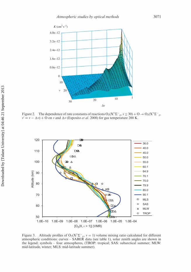
the new model of rate constants (Esposito et al. 2008) was used for the first time.This model describes not only the total quenching, but also the intermolecular V–Venergy exchange between upper and lower vibrational levels, when the lower vibra-tional levels are populated. The rate constant of this reaction strongly depends ontemperature. Figure 2 shows the dependence of rate constants of these reactions onv and �v. Detailed calculations of altitude profile O2(X3�−

g, v) concentrations fordifferent vibrational levels up to v ≤ 35 using the updated YM-2006 model werepresented in Yankovsky and Babaev (2011).

Lopez-Puertas et al. (1995) estimated that in the whole altitude range, the quan-tum yield of the vibrationally excited O2(X3�−

g, v = 1) per one photodissociatedO3 molecule was equal to 4. Utilizing the YM-2006 photolysis model enables us tocalculate the O2(X3�−

g, v = 1) population precisely for any given distribution ofatmospheric constituents and solar flux. We have used this model to calculate thealtitude profiles of the O2(X3�−

g, v) vibrational level populations for a number oftest cases (see figure 3). The purpose of this test was to verify the model for varioussolar fluxes, so we have found 12 events in mid-latitudes (from 38.9◦ N to 47.7◦ N)during the summer solstice in the northern hemisphere in 2002 that cover the solarzenith angle θ z grid in the interval θ z = 36.0◦–90.1◦. The atmospheric conditions forthese runs were taken from SABER V1.07 satellite experiment dataset available athttp://saber.gats-inc.com/. The parameters of the SABER scans are listed in table 1.

We also calculated the altitude profiles of O2(X3�−g, v = 1) concentration for

four typical atmospheric scenarios selected for the summer solstice in the northernhemisphere: subarctic summer (SAS: 70◦ N; θ z = 46.5◦), mid-latitude summer (MLS:40◦ N; θ z = 16.5◦), tropics (TROP: 0◦; θ z = 23.5◦) and mid-latitude winter (MLW:40◦ S; θ z = 63.5◦). We did not select the subarctic winter scenario since high latitudesin the southern hemisphere are not illuminated by the Sun during this season. Themain difference between these atmospheric scenarios is the temperature profile that

Dow

nloa

ded

by [

Tul

ane

Uni

vers

ity]

at 0

4:46

21

Sept

embe

r 20

13

Atmospheric studies by optical methods 3071

K (cm3 s–1)

4.0e–12

3.2e–12

2.4e–12

1.6e–12

0.8e–12

0

10

20

30 20 10

Δv

1

v

Figure 2. The dependence of rate constants of reactions O2(X3�−g, v ≤ 30) + O → O2(X3�−

g,v′ = v − �v) + O on v and �v (Esposito et al. 2008) for gas temperature 200 K.

36.0

40.0

45.0

50.0

55.0

60.1

64.9

70.1

75.0

79.9

85.0

90.1

MLS

SAS

MLW

TROP

50

60

70

80

Altitude (

km

)

90

100

110

120

[O2(X, v = 1)] (VMR)

1.0E–10 1.0E–09 1.0E–08 1.0E–07 1.0E–06 1.0E–05 1.0E–04

Figure 3. Altitude profiles of O2(X3�−g, v = 1) volume mixing ratio calculated for different

atmospheric conditions: curves – SABER data (see table 1), solar zenith angles are shown inthe legend; symbols – four atmospheres, (TROP: tropical; SAS: subarctical summer; MLW:mid-latitude, winter; MLS: mid-latitude summer).

Dow

nloa

ded

by [

Tul

ane

Uni

vers

ity]

at 0

4:46

21

Sept

embe

r 20

13

3072 V. Yankovsky et al.

Table 1. TIMED/SABER events selected for test runs.

Event Latitude (◦) Longitude (◦) Date θ z (◦)

29_01305 42.2 286.6 5 March 2002 70.0831_01378 42.7 297.2 10 March 2002 60.0732_01218 47.7 259.9 27 February 2002 85.0335_01238 41.1 129.1 01 March 2002 79.8936_01278 44.4 228.7 04 March 2002 75.0436_01468 43.3 251.1 16 March 2002 49.9737_01337 41.2 222.1 08 March 2002 64.9438_01176 42.6 209.1 25 February 2002 90.0738_01408 40.9 281.7 12 March 2002 55.0038_01491 34.2 47.0 18 March 2002 39.9939_01480 38.9 316.7 17 March 2002 45.0040_01498 30.2 235.5 18 March 2002 36.01

enables the study of the temperature-dependent effects in the model, including thethermal radiation effects. An important consequence of temperature profile variationfrom model to model is the pressure difference that leads to changes in optical depthsfor certain altitudes, which is important for photolysis rates calculations. We haveused temperature, total density, O2 and N2 VMR profiles obtained from the MSIS-E-90 model available online (http://omniweb.gsfc.nasa.gov/vitmo/msis_vitmo.html)for the summer solstice of 2002. The other atmospheric constituents needed for thecalculations (O3, O(1D), O(3P)) were taken from the corresponding zonal averages ofSABER for the same time of the year.

Figure 3 shows the altitude profiles of O2(X3�−g, v = 1) concentration for 12

SABER events listed in table 1 and for four typical atmospheric scenarios. As onecan see, all the profiles are close to each other for all the cases, except for the twilightone (θ z = 90.1o). In accordance with the reaction in equation (11), the enhancement ofthe O2(X3�−

g, v = 1) concentration below 78 km is connected with a sharp decreaseof atomic oxygen abundance below this altitude at twilight.

4. Parameterization of O2(X3�−g, v = 1) production

The calculation of O2(X3�−g, v = 1) concentration using the whole YM-2006 model

is a complicated task so we suggest a parameterization, namely, the total RQO of theO2(X3�−

g, v = 1) production.The RQO for the O2(X3�−

g, v = 1) level production due to ozone photolysis in theHartley, Huggins, Chappuis and Wulf bands (200–900 nm) is defined by the followingexpression:

RQO = [O2(X,v = 1)] Q(O2(X,v = 1)){JHartley + JChappuis + JHuggins + JWulf} [O3]

(12)

where [O2(X, v = 1)] is the O2(X3�−g, v = 1) concentration calculated in accor-

dance with the YM-2006 model without the contribution of O2 photolysis, Q(O2(X,v = 1)) is a factor of O2(X3�−

g, v = 1) quenching in collisions with N2, O2 and O(3P),and JHartley, JChappuis, JHuggins and JWulf are the ozone photodissociation rates for thecorresponding bands.

Dow

nloa

ded

by [

Tul

ane

Uni

vers

ity]

at 0

4:46

21

Sept

embe

r 20

13

Atmospheric studies by optical methods 3073

We stress here that in the RQO approach, we take into account the O2(X3�−g, v)

formation, not only in the direct processes of O3 photolysis, but also in the processesof energy transfer from O2(b1�+

g, v) and O2(a1�g, v) to O2(X3�−g, v) (see figure 1).

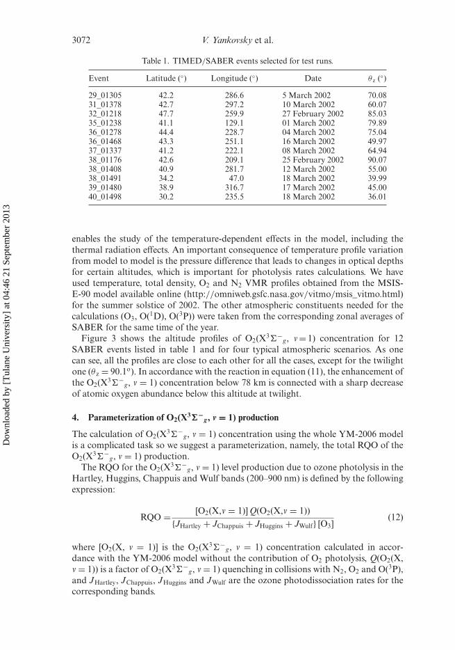
Figure 4 shows the RQO profiles in the MLT calculated for the same 12 test cases asin §3 (see table 1). As one can see, the altitude profiles of RQO for the 12 events ofTIMER/SABER overlap, fitting the 3σ confidence interval. The important findingmade in this study is the independence of RQO on latitude, longitude and solar zenithangle (figure 4), which enables us to tabulate it or to create a universal formula for itscalculation.

We suggest the following analytic formula for RQO parameterization depending onpressure in the interval from 1 mb to 2 × 10–5 mb:

RQO = exp(A + B(ln(p))2 + Cp), (13)

where A = 2.1370 ± 0.0328, B = −0.0366 ± 0.00207 and C = −0.1099 ± 0.0720are the parameterization coefficients, and p is the pressure in mb. This formula fitsthe RQO with the coefficient of determination r2 = 0.9916 and gives a fit standarderror equal to 0.2741 (see figure 4). We also tested the RQO parameterization for thefour above-mentioned typical atmospheric scenarios selected for the summer solsticein the northern hemisphere. It was found that the calculated RQO profiles for thesefour test atmospheric models are close (within the 3σ limits shown in figure 4) to theRQO calculated in accordance with the analytical formula of equation (13). It shouldbe noted that the RQO parameterization is applicable for calculations of O2(X3�−

g,v = 1) pumping in the altitude interval 50–90 km. Above 90 km, the role of O2

photolysis in the O2(X3�−g, v = 1) formation must be taken into account and the full

YM-2006 model should be used for calculations of O2(X3�−g, v = 1) concentration

(see figures 1 and 3).

RQ

O

10.0

8.0

6.0

4.0

2.0

0.01.0E–05 1.0E–04 1.0E–03 1.0E–02

p (mb)

1.0E–01 1.0E+00

Figure 4. Resulting quantum output production of O2(X3�−g, v = 1) (RQO) calculated for O3

photolysis in Hartley, Huggins, Chappuis and Wulf bands (200–900 nm) in the mesosphere andlower thermosphere. Black dots: RQO calculated for conditions of SABER data (see table 1);thick red line: RQO parameterization, equation (13); thin red lines: parameterization confidenceinterval 3σ ; symbols: RQO calculated for four atmospheric models (MLS, SAS, MLW, TROP).Symbols for atmospheric models are the same as in figure 3.

Dow

nloa

ded

by [

Tul

ane

Uni

vers

ity]

at 0

4:46

21

Sept

embe

r 20

13

3074 V. Yankovsky et al.

5. Applications of RQO to H2O retrieval in the mesosphere

We estimated the population of H2O(010) and O2(X3�−g, v = 1) and tested the

effects of the RQO parameterization using the Accelerated Lamda Iterations forAtmospheric Radiation and Molecular Spectra (ALI-ARMS) research code (seeKutepov et al. (1998), Gusev and Kutepov (2003) and references therein) that solvesthe non-LTE multi-level problem for an arbitrary number of molecular levels in theatmosphere by iterative solving of a set of statistical equilibrium equations and theradiative-transfer equations. For these calculations, the code was modified to includea ‘source’ member to the statistical equilibrium equation describing the populationand depopulation of the O2(X3�−

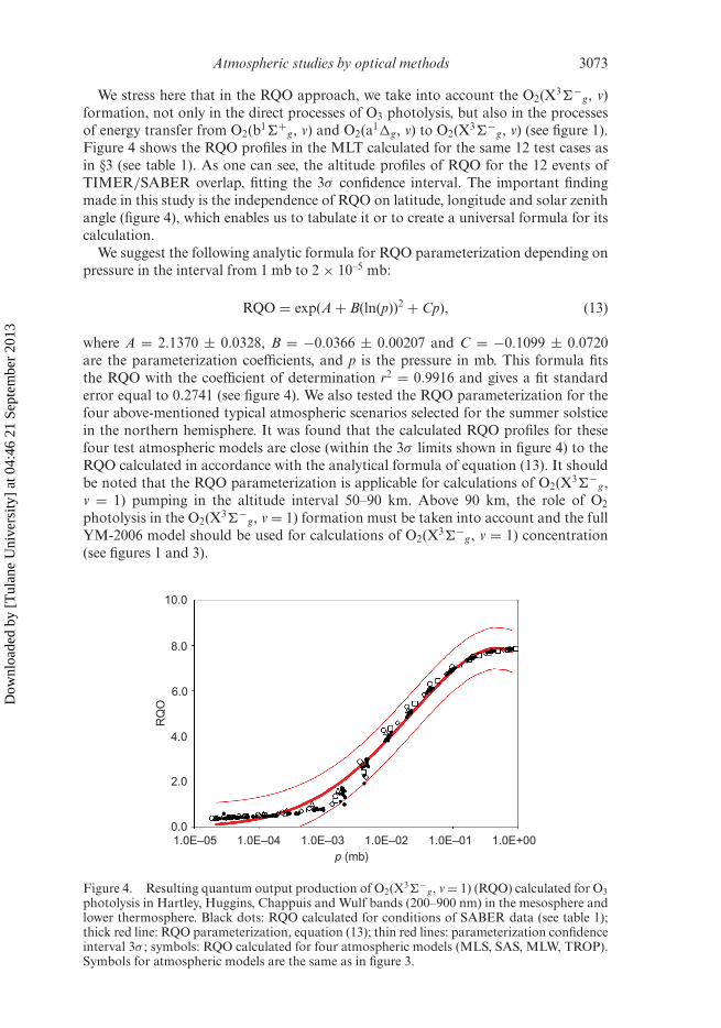
g, v = 1) level. The other atmospheric componentsthat were included to the non-LTE task are: H2O (1 isotope, 14 vibrational levels),CO2 (5 isotopes, 60 vibrational levels), N2 (1 isotope, 7 vibrational levels), O(3P) andO(1D). In figure 5, we demonstrate the significance of the process (2) for the vibra-tional kinetics of the H2O molecule. Figure 5 shows the ratio of H2O (010) populationcalculated for the case of H2O(v1, v2, v3)–O2(X3�−

g, v = 1) V–V coupling to H2O(010) population obtained in the case when the reaction (3) is not taken into accountfor the four atmospheric models.

As one can see from figure 5, below 70 km, taking into account the V–V energyexchange between O2(X3�−

g, v = 1) and H2O(010) (2) leads to a 2–12% increase ofthe H2O(010) level population. The most important influence of processes (3) on thepopulation of 010 is connected with deactivation of vibrational levels 010, 020, 030,110, 011, 040, 120 and 021 at near-resonance V–V energy exchange with O2(X3�−

g,v = 1) above 70 km, which leads to a decrease of the 010 level population from 45%to 75% at 85 km, in comparison with the population of 010 calculated without takingthis process into account.

140

SAS

MLS

TROP

MLW

120

100

Altitude (

km

)

80

60

40

200.2 0.4 0.6 0.8

O2 (X, v = 1) H2O (010)

H2O (010) coupled with O2 (X, v = 1)/H2O uncoupled

1 1.2

Figure 5. The ratio of H2O(010) population calculated for four atmospheric models (MLS,SAS, MLW, TROP), taking into account the processes of intermolecular quasi-resonance (V–V)energy exchange between O2(X3�−

g, v = 1) and H2O(v1, v2, v3) to H2O(010) populationcalculated without taking these processes into account.

Dow

nloa

ded

by [

Tul

ane

Uni

vers

ity]

at 0

4:46

21

Sept

embe

r 20

13

Atmospheric studies by optical methods 3075

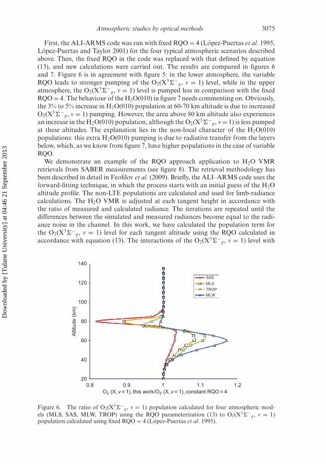
First, the ALI-ARMS code was run with fixed RQO = 4 (Lopez-Puertas et al. 1995,Lopez-Puertas and Taylor 2001) for the four typical atmospheric scenarios describedabove. Then, the fixed RQO in the code was replaced with that defined by equation(13), and new calculations were carried out. The results are compared in figures 6and 7. Figure 6 is in agreement with figure 5: in the lower atmosphere, the variableRQO leads to stronger pumping of the O2(X3�−

g, v = 1) level, while in the upperatmosphere, the O2(X3�−

g, v = 1) level is pumped less in comparison with the fixedRQO = 4. The behaviour of the H2O(010) in figure 7 needs commenting on. Obviously,the 3% to 5% increase in H2O(010) population at 60-70 km altitude is due to increasedO2(X3�−

g, v = 1) pumping. However, the area above 80 km altitude also experiencesan increase in the H2O(010) population, although the O2(X3�−

g, v = 1) is less pumpedat these altitudes. The explanation lies in the non-local character of the H2O(010)populations: this extra H2O(010) pumping is due to radiative transfer from the layersbelow, which, as we know from figure 7, have higher populations in the case of variableRQO.

We demonstrate an example of the RQO approach application to H2O VMRretrievals from SABER measurements (see figure 8). The retrieval methodology hasbeen described in detail in Feofilov et al. (2009). Briefly, the ALI–ARMS code uses theforward-fitting technique, in which the process starts with an initial guess of the H2Oaltitude profile. The non-LTE populations are calculated and used for limb-radiancecalculations. The H2O VMR is adjusted at each tangent height in accordance withthe ratio of measured and calculated radiance. The iterations are repeated until thedifferences between the simulated and measured radiances become equal to the radi-ance noise in the channel. In this work, we have calculated the population term forthe O2(X3�−

g, v = 1) level for each tangent altitude using the RQO calculated inaccordance with equation (13). The interactions of the O2(X3�−

g, v = 1) level with

Altitude (

km

)

140

120

100

80

60

40

200.8 0.9 1 1.1 1.2

SAS

MLS

TROP

MLW

O2 (X, v = 1), this work/O2 (X, v = 1), constant RQO = 4

Figure 6. The ratio of O2(X3�−g, v = 1) population calculated for four atmospheric mod-

els (MLS, SAS, MLW, TROP) using the RQO parameterization (13) to O2(X3�−g, v = 1)

population calculated using fixed RQO = 4 (López-Puertas et al. 1995).

Dow

nloa

ded

by [

Tul

ane

Uni

vers

ity]

at 0

4:46

21

Sept

embe

r 20

13

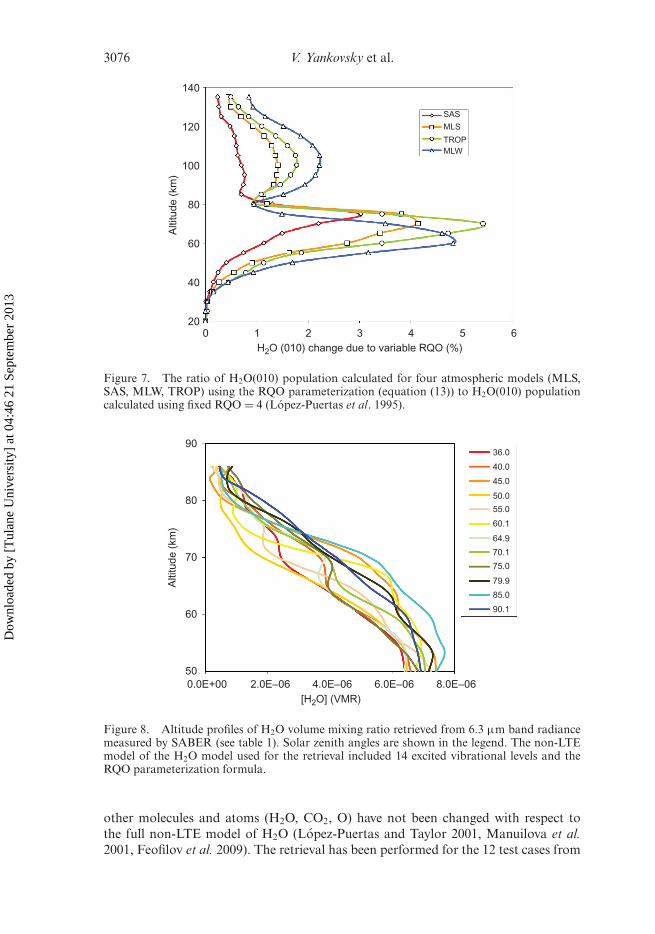
3076 V. Yankovsky et al.

SAS

MLS

TROP

MLW

Altitude (

km

)

140

120

100

80

60

40

200 1 2 3 4 5 6

H2O (010) change due to variable RQO (%)

Figure 7. The ratio of H2O(010) population calculated for four atmospheric models (MLS,SAS, MLW, TROP) using the RQO parameterization (equation (13)) to H2O(010) populationcalculated using fixed RQO = 4 (López-Puertas et al. 1995).

36.0

40.0

45.0

50.0

55.0

60.1

64.9

70.1

75.0

79.9

85.0

90.1

Altitude (

km

)

50

60

70

80

90

[H2O] (VMR)

0.0E+00 2.0E–06 4.0E–06 6.0E–06 8.0E–06

Figure 8. Altitude profiles of H2O volume mixing ratio retrieved from 6.3 µm band radiancemeasured by SABER (see table 1). Solar zenith angles are shown in the legend. The non-LTEmodel of the H2O model used for the retrieval included 14 excited vibrational levels and theRQO parameterization formula.

other molecules and atoms (H2O, CO2, O) have not been changed with respect tothe full non-LTE model of H2O (Lopez-Puertas and Taylor 2001, Manuilova et al.2001, Feofilov et al. 2009). The retrieval has been performed for the 12 test cases from

Dow

nloa

ded

by [

Tul

ane

Uni

vers

ity]

at 0

4:46

21

Sept

embe

r 20

13

Atmospheric studies by optical methods 3077

table 1. As one can see in figure 8, the absolute values of the H2O VMR retrieved inthis approach are in agreement with other measurements (Nedoluha et al. 2007). Theerror bars for the retrievals shown in figure 8 are ∼10% at and below 70 km, 20%at 80 km and 30% at 85 km (Feofilov et al. 2009). Taking into account the retrievaluncertainty and temporal and spatial variability of the water vapour, one may specu-late that figure 8 shows no dependence of H2O VMR on θ z. This is in agreement withthe long (20–30 hours) photochemical lifetime of water vapour in the altitude rangeconsidered (Brasseur and Solomon 2005). Summarizing, the RQO approach appliedto H2O VMR retrievals from SABER measurements provides reliable results at nocomputational cost.

6. Conclusions

We have updated the model of electronic-vibrational kinetics of the O2 and O3 pho-todissociation in the MLT by including the most recent estimate of the quenching rateof {O2(X3�−

g, v = 1) + O2} and {O2(X3�−g, v ≤ 30) + O}. The latter process is

extremely important for O2(X3�−g, v ≤ 30) vibrational de-excitation, so we used a

model that not only calculates the total quenching rate, but also describes the inter-molecular V–V energy exchange between upper and lower vibrational levels, when thelower vibrational levels O2(X3�−

g, v) are populated. As a result, an updated YM-2006 model enables one to calculate the altitude dependence of the populations of 35vibrational states of O2 molecules in the ground electronic state.

We have described the RQO approach for estimating the O2(X3�−g, v = 1) vibra-

tional level pumping and suggested a parameterization of the RQO that can be usedin the non-LTE models of trace gas molecules in the MLT. The RQO describes thenet effect of the O2(X 3�−

g, v = 1) level production due to ozone photolysis in theHartley, Huggins, Chappuis and Wulf bands (200–900 nm). We have studied the RQObehaviour in the latitude interval from 70◦ N to 70◦ S and for θ z up to 90◦ with respectto different atmospheric conditions, and found that it depends strongly on altitude,and weakly on the solar zenith angle, latitude, longitude and season.

We have demonstrated RQO approach applications to H2O VMR retrievals from6.3 µm SABER radiometric measurements. The RQO approach has been incorpo-rated into the H2O non-LTE model in the SABER operational code, and will be usedfor H2O retrievals in the next release of SABER data.

AcknowledgementsWe are grateful to Dr Fabrizio Esposito and his colleagues from the Istituto diMetodologie Inorganiche e dei Plasmi, Bari, Italy for providing the code of cal-culation of reaction (11) rate constant. The study was supported by grant RFBRno. 09-05-00 694-a.

ReferencesBRASSEUR, G.P. and SOLOMON S.C., 2005, Aeronomy of the Middle Atmosphere (Dordrecht,

The Netherlands: Springer).ESPOSITO, F., ARMEHISE, I., CAPITTA, G. and CAPITELLI, M., 2008, O–O2 state-to-state vibra-

tional relaxation and dissociation rates based on quasiclassical calculations. ChemicalPhysics, 351, pp. 91–98.

FEOFILOV, A.G., KUTEPOV, A.A., PESNELL, W.D., GOLDBERG, R.A., MARSHALL, B.T.,GORDLEY, L.L., GARCÍA–COMAS, M., LÓPEZ-PUERTAS, M., MANUILOVA, R.O.,

Dow

nloa

ded

by [

Tul

ane

Uni

vers

ity]

at 0

4:46

21

Sept

embe

r 20

13

3078 V. Yankovsky et al.

YANKOVSKY, V.A., PETELINA, S.V. and RUSSELL III, J.M., 2009, DaytimeSABER/TIMED observations of water vapor in the mesosphere: retrieval approachand first results. Atmospheric Chemistry and Physics, 9, pp. 8139–8158.

GUSEV, O.A. and KUTEPOV, A.A., 2003, Non-LTE gas in planetary atmospheres. StellarAtmosphere Modelling, 288, pp. 318–330.

HUESTIS, D.L., 2006, Vibrational energy transfer and relaxation of O2 and H2O#. Journal ofPhysical Chemistry A, 110, pp. 6638–6642.

KALOGERAKIS, K.S., PEJAKOVIC, D.A., COPELAND, R.A. and SLANGER, T.G., 2005, Relativeyield of O2(b1�+

g, v = 0 and 1) in O(1D) + O2 collisions. EOS Transactions AGU ,86(52), AGU Fall Meeting, SA11A-0220, 5–9 December 2005, San Francisco, CA.

KUTEPOV, A.A., GUSEV, O.A. and OGIBALOV, V.P., 1998, Solution of the non-LTE problem formolecular gas in planetary atmospheres: superiority of accelerated lambda iteration.Journal of Quantitative Spectroscopy and Radiative Transfer, 60, pp. 199–220.

LÓPEZ-PUERTAS, M. and TAYLOR, F.W., 2001, Non-LTE Radiative Transfer in the Atmosphere(River Edge, NJ: World Scientific Publishing Co.).

LÓPEZ-PUERTAS, M., ZARAGOZA G., KERRIDGE, B.J. and TAYLOR, F.W., 1995, Non-local ther-modynamic equilibrium model for H2O 6.3 and 2.7 µm bands in the middle atmosphere.Journal of Geophysical Research, D100, pp. 9131–9147.

MANUILOVA, R.O., YANKOVSKY, V.A., GUSEV, O.A., KUTEPOV, A.A., SULAKSHINA, O.N. andBORKOV, YU.G., 2001, Non-equilibrium middle atmosphere radiation in the infraredro-vibrational water vapor bands. Atmospheric and Oceanic Optics, 14, pp. 864–867.

MATSUMI, Y. and KAWASAKI, M., 2003, Photolysis of atmospheric ozone in the ultravioletregion. Chemical Reviews, 103, pp. 4767–4781

MLYNCZAK, M.G., SOLOMON, S.C. and ZARAS, D.S., 1993, An updated model for O2(a1�g)concentrations in the mesosphere and lower mesosphere and implications for remotesensing of ozone at 1.27 µm. Journal of Geophysical Research, D98, pp. 18 639–18 648.

NEDOLUHA, G.E., GOMEZ, R.M., HICKS, B.C., BEVILACQUA, R.M., RUSSELL III, J.M.,CONNOR, B.J. and LAMBERT, A., 2007, A comparison of middle atmospheric watervapor as measured by WVMS, EOS–MLS, and HALOE. Journal of GeophysicalResearch, 112, D24S39, doi: 10.1029/2007JD008757.

OLEMSKOY, I.V., 2006, Updating of algorithm of allocation structural features. Vestnnik Sankt-Peterburgskogo Universiteta. Seriya 10: Prikladnaya. Matemematika, 1, pp. 55–64.

SONNEMANN, G. R., GRYGALASHVYLY, M. and BERGER, U., 2005, Autocatalytic water vaporproduction as a source of large mixing ratios within the middle to upper mesosphere.Journal of Geophysical Research, 110, D15303, doi: 10.1029/2004JD005593.

SPARKS, R.K., CARLSON, L.R., SNOBATAKE, K., KOWALCZYK, M.L. and LEE, Y.T., 1980,Ozone photolysis: a determination of the electronic and vibrational state distributionsof primary products. Journal of Chemical Physics, 72, pp. 1401–1402.

THELEN, M.A., GEJO, T., HARRISON, J.A. and HUBER, J.R., 1995, Photodissociation of ozonein the Hartley band: fluctuation of the vibrational state distribution in the O2(a1�g, v)fragment. Journal of Chemical Physics, 103, pp. 7946–7955.

VALENTINI, J.J., GERRITY, D.P., PHILLIPS, D.L., NIEH, J.-C. and TABOR, K.D., 1987, CARSspectroscopy of O2(a1�g) from the Hartley band photodissociation of O3: dynamics ofthe dissociation. Journal of Chemical Physics, 86, pp. 6745–6756.

YANKOVSKY, V.A. and BABAEV, A.S., 2011, Photolysis of O3 in the Hartley, Huggins, Chappuisand Wulf bands in the middle atmosphere: vibrational kinetics of oxygen moleculesO2(X3�−

g, v ≤ 35). Atmospheric and Oceanic Optics, 24, pp. 6–16.YANKOVSKY, V.A. and MANUILOVA, R.O., 2006, Model of daytime emissions of electronically

vibrationally excited products of O3 and O2 photolysis: application to ozone retrieval.Annales Geophysicae, 24, pp. 2823–2839.

YANKOVSKY, V.A., KULESHOVA, V.A., MANUILOVA, R.O. and SEMENOV, A.O., 2007, Retrievalof total ozone in the mesosphere with a new model of electronic vibrational kinetics ofO3 and O2 photolysis products. Atmospheric and Oceanic Physics, 43, pp. 514–525.

YEE, J.-H., CAMERON, G.E. and KUSNIERKIEWICZ, D.Y., 1999, Overview of TIMED. SPIE,3756, pp. 244–254.

Dow

nloa

ded

by [

Tul

ane

Uni

vers

ity]

at 0

4:46

21

Sept

embe

r 20

13