
Measurement of the photon polarization using B0 s ϕγ at LHCb
214
HAL Id: tel-01176223 https://tel.archives-ouvertes.fr/tel-01176223 Submitted on 15 Jul 2015 HAL is a multi-disciplinary open access archive for the deposit and dissemination of sci- entific research documents, whether they are pub- lished or not. The documents may come from teaching and research institutions in France or abroad, or from public or private research centers. L’archive ouverte pluridisciplinaire HAL, est destinée au dépôt et à la diffusion de documents scientifiques de niveau recherche, publiés ou non, émanant des établissements d’enseignement et de recherche français ou étrangers, des laboratoires publics ou privés. Measurement of the photon polarization using B0 s → ϕγ at LHCb Mostafa Hoballah To cite this version: Mostafa Hoballah. Measurement of the photon polarization using B0 s → ϕγ at LHCb. Other [cond- mat.other]. Université Blaise Pascal - Clermont-Ferrand II, 2015. English. NNT: 2015CLF22555. tel-01176223
Transcript of Measurement of the photon polarization using B0 s ϕγ at LHCb
HAL Id: tel-01176223https://tel.archives-ouvertes.fr/tel-01176223
Submitted on 15 Jul 2015
HAL is a multi-disciplinary open accessarchive for the deposit and dissemination of sci-entific research documents, whether they are pub-lished or not. The documents may come fromteaching and research institutions in France orabroad, or from public or private research centers.
L’archive ouverte pluridisciplinaire HAL, estdestinée au dépôt et à la diffusion de documentsscientifiques de niveau recherche, publiés ou non,émanant des établissements d’enseignement et derecherche français ou étrangers, des laboratoirespublics ou privés.
Measurement of the photon polarization using B0 s →ϕγ at LHCbMostafa Hoballah
To cite this version:Mostafa Hoballah. Measurement of the photon polarization using B0 s → ϕγ at LHCb. Other [cond-mat.other]. Université Blaise Pascal - Clermont-Ferrand II, 2015. English. �NNT : 2015CLF22555�.�tel-01176223�
Numéro d’Ordre : DU 2555
EDSF : 817
PCCF T 1502
UNIVERSITÉ BLAISE PASCAL DECLERMONT-FERRAND
(U.F.R. Sciences et Technologies)
ÉCOLE DOCTORALE DES SCIENCES FONDAMENTALES
THÈSE
présentée pour obtenir le grade de
DOCTEUR D’UNIVERSITÉSpécialité : PHYSIQUE des PARTICULES
par
Mostafa HOBALLAH
Measurement of the photon polarization using B0s → φγ at LHCb.
Thèse soutenue publiquement le 03 Mars 2015, devant la commission d’examen:
M. A. FALVARD Président du jury
M. A. A. GALLAS TORREIRA Rapporteur
Mme. E. TOURNFIER Rapporteur
M. K. TRABELSI Examinateur
M. O. DESCHAMPS Directeur de thèse
M. P. PERRET Directeur de thèse


i

Résumé
Cette thèse est dédiée à l’étude des désintégrations B0s → φγ au LHCb afin de mesurer
la polarisation du photon . Au niveau des quarks, ces désintégrations procèdent viaune transition pingouin b → sγ et sont sensibles aux eventuelles contributions virtuellesde Nouvelle Physique. La mesure de la polarisation du photon permet de tester lastructure V − A du couplage du Modèle Standard dans les processus des diagrammesde boucles de pingouin. Cette mesure peut être réalisée en étudiant le taux de dés-intégration dépendant du temps des mésons B. Une analyse délicate a été faite pourcomprendre la distribution du temps propre et l’acceptance de sélection qui affecte cettedistribution. Afin de contrôler l’acceptance de temps propre, des méthodes basées surles données ont été développées. Plusieurs stratégies utilisées dans la mesure de la po-larisation des photons sont introduites et des résultats préliminaires sont présentés. Deplus, une étude de certains effets systématiques est discutée. Dans le cadre de l’étudedes désintégrations radiatives, une nouvelle procedure d’identification de photons a étédéveloppée et nous avons fourni un outil pour calibrer la performance de la variable deséparation photon/pion neutre sur la simulation. Ces outils sont d’intérêt général pourla collaboration LHCb et sont largement utilisés.
Mots clés: LHCb detector - Heavy Flavor Physics - Radiative Decays -Effective Field Theories - B0
s → φγ - Photon Polarization - Proper Time -Photon Identification - Photon/π0 separation.
iii


v

Abstract
This thesis is dedicated to the study of the photon polarization in B0s → φγ decays at
LHCb. At the quark level, such decays proceed via a b → sγ penguin transition andare sensitive to possible virtual contributions from New Physics. The measurement ofthe photon polarization stands also as a test of the V − A structure of the StandardModel coupling in the processes mediated by loop penguin diagrams. The measurementof the photon polarization can be done through a study of the time-dependent decayrate of the B meson. A delicate treatment has been done to understand the proper timedistribution and the selection acceptance affecting it. To control the proper time accep-tance, data driven control methods have been developed. Several possible strategies tomeasure the photon polarization are introduced and preliminary blinded results are pre-sented. A study of some of the systematic effects is discussed. In the context of studyingradiative decays, the author has developed a new photon identification procedure andhas provided a tool to calibrate the performance of the photon/neutral pion separationvariable on simulation. Those tools are of general interest for the LHCb collaborationand are widely used.
Keywords:
LHCb detector - Heavy Flavor Physics - Radiative Decays - Effective FieldTheories - B0
s → φγ - Photon Polarization - Proper Time - Photon Identifi-cation - Photon/π0 separation.
vii


Remerciements
My acknowledgements go to everyone who has contributed in some way to thedevelopment of this work. I begin by thanking the director of the LPC, Alain Falvard,for granting me the chance to prepare my thesis in good conditions.
I want to thank the région d’Auvergne for having financially supported this work duringthree years and also for having granted me extra financial support to participate to con-ferences and present my work.
I am so happy to have been part of the LHCb team in the LPC. I would like to thankall the members of the team especially Olivier Deschamps and Régis Lefevre who haveworked hard with me so as to elaborate this work and make it in a good condition. In thepast three years I have experienced the most difficult but also the most beautiful moments,memories that will stay engraved in my mind till the day I die.
I would like also to thank all the members of the radiative analysis working group in theLHCb collaboration your help is very well appreciated.
My fellow students and friends in the LPC, Ibrahim, Marouen, Mohamad, Jan.. I wouldlike to thank you for all your help and all your time that you have spent with me.Marouen, I will never forget all the times that we spent on the balcony smoking -mebeing as a passive smoker- those moments were the best moments of a working day.
Also, I am very grateful to Alain Falvard, Karim Trabelsi, Edwige Tournefier and Abra-ham Gallas for having accepted to be a part of my thesis jury.
ix

x
I am to mention my daughter Ilyana since her presence has made me realize more andmore the importance of my parents in my life. Since the day I knew she was coming Istarted to live a new kind of emotions, emotions that I knew my father has felt whenhe knew that I was coming, I can not just pass by such situation without realizing howmuch my parents cared about me and how much they sacrificed. Thanking them wouldnot express the enormous amount of gratitude that I have towards them. I can now feelhow much they are happy to see that their son has achieved something in this life.
On several unthought occasions your shadow would come to my mind flashing back aseries of beautiful memories that I have lived by your side. Your smile has given mea lot of energy when I was feeling stressed. I would like to thank you for having knewyou... Mariam.

1 �������� ������ ���� ������� �� ���� ������������ ������
� ���� !�� ��!��" #� �$� ���!��� �% �& �'�
`àffl ”m`affl f´a‹m˚i˜l¨l´e,`àffl M`a˚r˚i`a‹mffl,`àffl I˜l›y´a‹n`affl...
1. «Comme si la vie n’a jamais existé, et que la vie de l’au-delà est toujours là» , Hussain ibn Ali Ibn Abi Taleb. Quand Hussain ibn Ali IbnAbi Taleb s’est rapproché de sa mort, il s’apercevait plus que jamais que le temps qu’il a passé en vie n’était qu’un voyage vers un autre mondeplus joli, et surtout, un monde éternel.

Contents
Introduction 1
1 The Electroweak interaction 3
1.1 The Standard Model . . . . . . . . . . . . . . . . . . . . . . . . . . . . . 4
1.2 Radiative B hadron decays . . . . . . . . . . . . . . . . . . . . . . . . . . 14
2 The LHCb 25
2.1 The LHC . . . . . . . . . . . . . . . . . . . . . . . . . . . . . . . . . . . 26
2.2 Data taking periods and operating conditions . . . . . . . . . . . . . . . 28
2.3 The LHCb detector . . . . . . . . . . . . . . . . . . . . . . . . . . . . . . 29
2.4 The LHCb trigger system . . . . . . . . . . . . . . . . . . . . . . . . . . 48
2.5 The LHCb luminosity measurements . . . . . . . . . . . . . . . . . . . . 52
2.6 The LHCb software . . . . . . . . . . . . . . . . . . . . . . . . . . . . . . 53
2.7 Data flow in LHCb . . . . . . . . . . . . . . . . . . . . . . . . . . . . . . 54
3 Photon reconstruction and identification 55
3.1 Photon reconstruction . . . . . . . . . . . . . . . . . . . . . . . . . . . . 56
3.2 π0 reconstruction . . . . . . . . . . . . . . . . . . . . . . . . . . . . . . . 59
3.3 Multivariate approaches . . . . . . . . . . . . . . . . . . . . . . . . . . . 60
3.4 Photon identification . . . . . . . . . . . . . . . . . . . . . . . . . . . . . 63
3.5 γ/π0 separation . . . . . . . . . . . . . . . . . . . . . . . . . . . . . . . . 76
4 The measurement of the photon polarization in B0s → φγ 87
4.1 Introduction . . . . . . . . . . . . . . . . . . . . . . . . . . . . . . . . . . 88
xiii
xiv CONTENTS
4.2 Signal and control channels selection . . . . . . . . . . . . . . . . . . . . 91
4.3 The proper time . . . . . . . . . . . . . . . . . . . . . . . . . . . . . . . . 102
4.4 Proper time acceptance study on MC . . . . . . . . . . . . . . . . . . . . 113
5 Preliminary results 131
5.1 Fit strategies . . . . . . . . . . . . . . . . . . . . . . . . . . . . . . . . . 132
5.2 Extracting τB0 with B0→ K∗(892)0γ events . . . . . . . . . . . . . . . . 135
5.3 Sensitivity on AΔ . . . . . . . . . . . . . . . . . . . . . . . . . . . . . . . 141
5.4 Systematic uncertainties study . . . . . . . . . . . . . . . . . . . . . . . . 153
5.5 Conclusions . . . . . . . . . . . . . . . . . . . . . . . . . . . . . . . . . . 161
Conclusion 163
Appendices 169
A B → V γ and B → V J/ψ time acceptance alignment 169
A.1 Kinematical basis of the procedure . . . . . . . . . . . . . . . . . . . . . 169
A.2 Alignment of the proper time acceptance . . . . . . . . . . . . . . . . . . 177
B Photon calibration 179
C Definition of the different variables used for selections 181


Introduction
The Standard Model (SM) of particle physics provides a successful interpretationof most of the observed phenomena. There are several theoretical or experimental openquestions as the origin of the mass hierarchy, the leptons family number, the electriccharge quantification, the existence of dark matter and the asymmetries in the universe.These open questions may suggest that more fundamental symmetries are at play andjustify the search for new phenomena beyond the standard model. This New Physicssearch can be done either by searching for new heavy particles or with precision valida-tion of the SM predictions.
The validity of the SM can be checked in many ways one of which is the study of bhadron decays. One of the main experiments that study b flavor is the LHCb at CERN.The b quark transitions proceeding via Flavor-Changing Neutral Current (FCNC) loopprocesses provide an efficient indirect probe for the search of new particles possibly prop-agating inside the virtual loops. Precision measurements in the flavor sector can help toobserve such NP effects.
One of the most promising probes of NP is the measurement of the photon polarizationin b → sγ penguin transitions. The photon in b → sγ is predominantly left handed inthe SM due to the left handed nature of the electroweak interactions. The right handedcomponent is suppressed by the ratio of ms/mb. The exact level of suppression dependson QCD effects where, for certain modes, diagrams with gluon emission can contribute tothe matrix element through their mixing. The measurement of the photon polarizationwould then aim at evaluating the fraction of right handed photons in hopes of findingdeviation from the SM.
1
2 Introduction
The determination of the photon polarization in b → sγ transitions is one of the im-portant measurement of the LHCb physics program. Measuring the photon polarizationcan be done through the measurement of the time dependent decay rate of B0
s → φγ.
This thesis introduces the analysis of the data collected by the LHCb detector duringthe 2011-2012 run I period in view of the first extraction of the photon polarization inthe time-dependent decay rate of the B0
s → φγ decays. This analysis results from acollaborative work that involves several institutes, the LPC Clermont, the EPFL Lau-sanne, the IFIC Valencia and Barcelona groups working in the Radiative sub-group ofthe Rare Decays working group of the LHCb collaboration. This document presents mypersonal contribution to the teamwork. The analysis not being yet finalized, some pre-liminary results on the ratio of left to right photon polarization amplitudes are discussed.
This document is organized as follows. The first chapter serves as an introduction to theStandard Model of particle physics. The phenomenology of b → sγ transition based onthe framework of effective field theories and Operator Product Expansion is introduced.An experimental overview with the recent results on radiative B decays are presented.
The second chapter introduces the LHCb detector at the LHC. The different sub-detectors are presented. Since the work presented in this thesis is focused on radiativedecays, care has been taken in explaining the calorimeter part of the detector for itsmajor role in reconstructing photons.
The photon being extremely important to reconstruct the final state of the decay, chapterthree has been dedicated to the reconstruction and identification of the photon. Theauthor is directly implicated in the development of the photon identification tools atLHCb.
Chapter four presents the analysis performed to extract the photon polarization fromB0
s → φγ.
Finally, chapter five presents the preliminary results.
Technical details are collected in the appendices.

Chapter 1
The Electroweak interaction
Contents1.1 The Standard Model . . . . . . . . . . . . . . . . . . . . . . . 4
1.1.1 The Lagrangian of the Standard Model . . . . . . . . . . . . . 5
1.1.2 Higgs sector . . . . . . . . . . . . . . . . . . . . . . . . . . . . . 9
1.2 Radiative B hadron decays . . . . . . . . . . . . . . . . . . . . 14
1.2.1 Effective field theories . . . . . . . . . . . . . . . . . . . . . . . 15
1.2.2 Experimental status . . . . . . . . . . . . . . . . . . . . . . . . 18
1.2.3 Radiative B decays at LHCb . . . . . . . . . . . . . . . . . . . 22
3
4 The Electroweak interaction
The present understanding of the fundamental interactions is summarized intothe so-called Standard Model of particle physics (SM). The later describes all knownphenomenology of elementary particles from very low energy scales up to the highestexperimental ones. Certain aspects of the SM have been tested with high precision andno significant deviation has been found. However, there are some phenomena which arenot explained within the SM such as neutrino masses and the hierarchy problem.In this chapter, the theoretical and the phenomenological framework is recalled. The SMof particle physics is briefly introduced followed by a description of the flavor changingneutral processes. Finally the radiative decay of interest is presented and the experimentalstatus is shown.
1.1 The Standard Model
The Standard Model of particle physics is a renormalizable quantum field theory basedon the gauge group SU(3)c×SU(2)L×U(1)Y where the SU(3)c is the gauge group of theQuantum Chromodynamics (QCD) part and SU(2)L × U(1)Y induces the electroweakinteraction. The gauge group has 12 generators corresponding to eight gluons for thestrong interaction, three weak bosons W± and Z0 and the photon mediating the elec-tromagnetic interaction.The matter fields, being the quarks and the leptons, are grouped into multiplets of thegauge group, i.e. they have to be assigned electroweak and strong quantum numbers.Parity violation in weak interactions is implemented by assigning different weak quan-tum numbers to left- and right-handed components of the matter fields. In other words,the left- and right-handed components of the quarks and leptons are associated withdifferent multiplets of the electroweak SU(2)L ⊗ U(1)Y group. The left-handed leptonsare grouped into doublets of SU(2)L in the following way:
Lj,L =
(νj
lj
)L
where lj ∈ {e, μ,τ }
where the subscript L means the left-handed projection of the spinor fields
ψL =1
2(1− γ5)ψ

1.1 The Standard Model 5
Similarly, for the quarks the assignment is
Qj,L =
(Uj
Dj
)L
where, assuming that there are six quarks and no more, Uj ∈ {u, c, t} are the up-typequarks with a charge Q = 2/3 and Dj ∈ {d, s, b} are the down-type quarks having acharge of −1/3.The right-handed quarks and leptons are singlets in the SM. Thus
Lj,R =(lj
)R
, QUj,R =
(Uj
)R
and QDj,R =
(Dj
)R
for the right handed leptons, up-type quarks and down-type quarks respectively. It isimportant to mention that the right-handed components are not sensitive to weak in-teractions. Only the left-handed group SU(2)L is gauged and yields the usual couplingsof the gauge bosons to the quarks and leptons.
The hypercharge assignment is determined in terms of the electric charge Q and thethird component of the weak isospin I3 quantum numbers,
Y = 2(Q− I3)
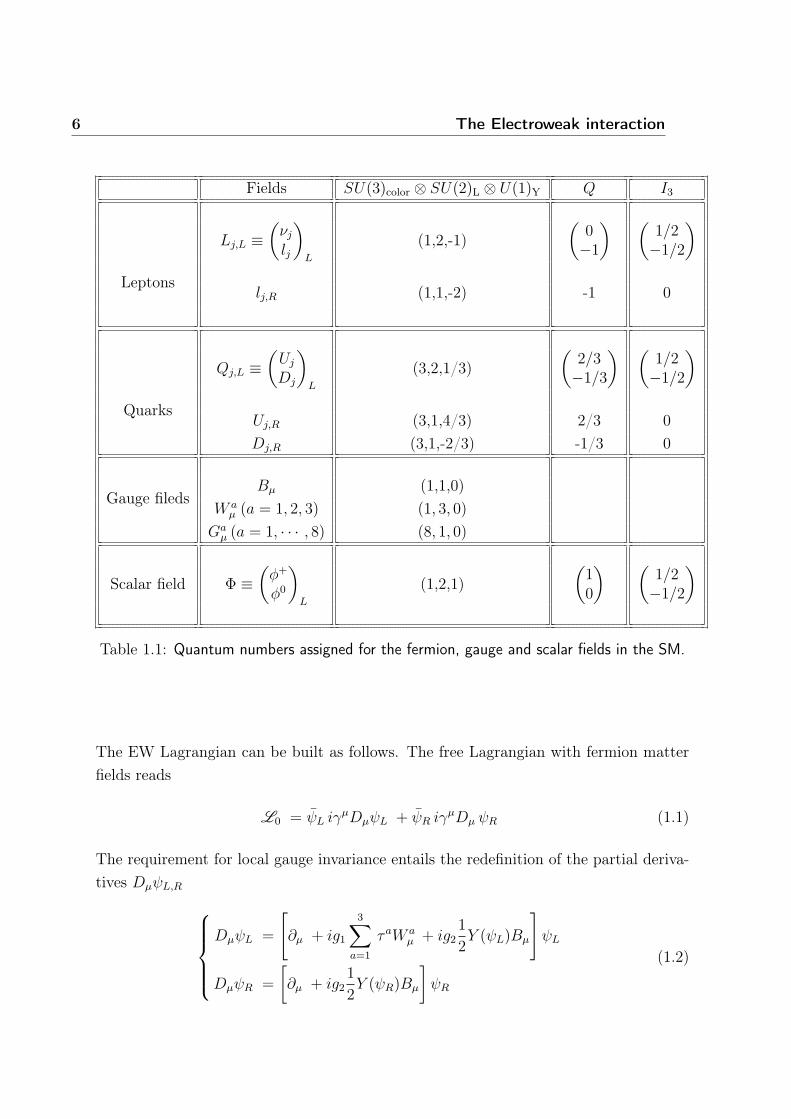
Table 1.1 shows the different behavior of the left- and right- handed particles underSU(2)L transformations where the left-handed particles are written as doublets and theright-handed ones as singlets. It also shows the quantum numbers assigned for thefermion, gauge and scalar fields in the SM.
1.1.1 The Lagrangian of the Standard Model
The SM gauge symmetry SU(3)c×SU(2)L×U(1)Y is spontaneously broken as SU(2)L×U(1)Y → U(1)Q. The electroweak theory, proposed by Glashow, Salam and Weinberg[1, 2] is a non-abelian theory based on SU(2)L × U(1)Y describing the electromagneticand weak interaction between quarks and leptons. In addition to the SU(2) generators,I± and I3, the hypercharge Y = 2(Q− I3), where Q is the electric charge, is introducedin order to accommodate the difference between the electric charges for the left-handeddoublets.
6 The Electroweak interaction
Fields SU(3)color ⊗ SU(2)L ⊗ U(1)Y Q I3
Lj,L ≡(νjlj
)L
(1,2,-1)(
0−1
) (1/2−1/2
)Leptons
lj,R (1,1,-2) -1 0
Qj,L ≡(Uj
Dj
)L
(3,2,1/3)(
2/3−1/3
) (1/2−1/2
)Quarks
Uj,R (3,1,4/3) 2/3 0Dj,R (3,1,-2/3) -1/3 0
Bμ (1,1,0)Gauge fileds
W aμ (a = 1, 2, 3) (1, 3, 0)
Gaμ (a = 1, · · · , 8) (8, 1, 0)
Scalar field Φ ≡(φ+
φ0
)L
(1,2,1)(10
) (1/2−1/2
)
Table 1.1: Quantum numbers assigned for the fermion, gauge and scalar fields in the SM.
The EW Lagrangian can be built as follows. The free Lagrangian with fermion matterfields reads
L0 = ψL iγμDμψL + ψR iγμDμ ψR (1.1)
The requirement for local gauge invariance entails the redefinition of the partial deriva-tives DμψL,R ⎧⎪⎪⎪⎨⎪⎪⎪⎩
DμψL =
[∂μ + ig1
3∑a=1
τaW aμ + ig2
1
2Y (ψL)Bμ
]ψL
DμψR =
[∂μ + ig2
1
2Y (ψR)Bμ
]ψR
(1.2)
1.1 The Standard Model 7
The two real numbers g1 and g2 are the couplings associated with SU(2) and U(1)
respectively, and Y is the U(1) hypercharge.Thus, four gauge fields are present: W a, corresponding to the three SU(2) generators,and B corresponding to U(1). Introducing the field strengths
Bμν = ∂μBν − ∂νBμ (1.3)
W Aμν = ∂μW
Aν − ∂νW
Aμ − g1εABCW
Bμ WC
ν (1.4)
where εABC is the totally antisymmetric Levi-Civita tensor, one can then construct thekinetic Lagrangian of the gauge fields
Lkin = −1
4BμνB
μν − 1
4
3∑a=1
W aμνW
aμν (1.5)
Gauge symmetry forbids mass terms for the gauge bosons and the fermions. Thus, theSU(2)L ⊗ U(1)Y Lagrangian contains only massless fields.
The interactions of the fermions with the gauge bosons are given by
Lint = −g1ψLγμWμψL − g2 Bμ
∑ψj∈�j , ν�j ,
Quj , Q
dj
y(ψj)ψjγμψj (1.6)
where Wμ(x) ≡ τaW aμ (x)/2 and y(ψj) ≡ YW (ψj)/2.
However, the SU(2)L⊗U(1)Y Lagrangian cannot describe the observed dynamics becausethe gauge bosons and the fermions are still massless.
The QCD Lagrangian can be built as follows. The free Lagrangian with massless quarkfields reads
L 0q + L I
Aq = ψi (iγμ(Dμ)ij)ψj (1.7)
where L 0q and L I
Aq stand for the free quark Lagrangian and quark-gluon interactionLagrangian respectively.To take into account the effect of a local color gauge transformation on the dynamics of
8 The Electroweak interaction
the quark field, the covariant derivative is defined as
Dμψi =
[∂μ + igs
1
2λaA
aμ
]ψi (1.8)
where gs is the coupling constant of the strong interaction, λa are the Gell-Mann gener-ators of the SU(3) group and Aμ represents the gluon field.
The gauge invariant gluon field strength tensor is defined as
Gaμν = ∂μA
aν − ∂νA
aμ − gsf
abcAbμ A
cν (1.9)
where fabc are the structure constants of SU(3) group. The dynamical term for gluonscan be expressed by the gauge and Lorentz invariant Lagrangian density defined as
L 0A + L I
A = −1
2Tr(GμνG
μν) (1.10)
where Gμν =1
2λaGa,μν and Tr stands for Trace. L 0
A and L IA are the free gluon and
gluon-gluon interaction Lagrangians.With some mathematical manipulation, this dynamical term can be reduced to the form
L 0A + L I
A = −1
4Ga
μνGa,μν (1.11)
developing this using 1.9 one will arrive to the form
L 0A + L I
A = −1
4
(∂μA
aν − ∂νA
aμ
)2 −gsfabc∂μAν
aAbμA
cν
− g2s4fabcfab′c′A
bμA
cνA
b′μAc′ν(1.12)
it can be noticed that besides the kinetic term for the free gluons, the Lagrangiancontains three- and four- gluon coupling terms.
to summarize, the QCD Lagrangian can be written as
LQCD = L 0q + L 0
A + L IAq + L I
A (1.13)
For completeness, it is important to mention that the QCD Lagrangian has two extraterms incorporating “ghost” fields and their interactions. Ghost fields were introduced byFaddeev and Popov into gauge quantum field theories to maintain the consistency of the
1.1 The Standard Model 9
path integral formulation. The gluon propagator was singular, could not be defined, andfixing a gauge, by introducing the Faddeev-Popov determinant, lead to the emergenceof those purely mathematical, and non-physical, objects, hence the naming “ghosts”.
To this extent the SM Lagrangian can be defined as the combination of 1.13 , 1.1, 1.5and 1.6.
1.1.2 Higgs sector
The origin of mass in the SM is a consequence of the spontaneous symmetry breaking(SSB) of the SU(2)L ⊗ U(1)Y triggered by the Higgs mechanism (developed by Higgs,Brout, Englert, Guralnik, Hagen and Kibble) [3–6]. Consider an SU(2)L doublet ofcomplex scalar fields
φ ≡(φ(+)
φ(0)
)(1.14)
The scalar Lagrangian is
LS = (Dμφ)† Dμφ− μ2φ†φ − h
(φ†φ)2
(h > 0, μ2 < 0) (1.15)
with the covariant derivative
Dμφ =[∂μ + ig1Wμ + ig2y(φ)B
μ]φ with y(φ) =
1
2(1.16)
The Lagrangian LS is invariant under local SU(2)L ⊗ U(1)Y transformations.There is an infinite set (S ) of degenerate states with minimum energy, satisfying
〈0 |φ(0) | 0〉 =
√−μ2
2h≡ v√
2(1.17)
where v is the vacuum expectation value (VEV) of the neutral scalar. Since the electriccharge is conserved, the VEV of φ+ must vanish. Once the system has chosen a particularstate belonging to (S ), the SU(2)L ⊗ U(1)Y symmetry is spontaneously broken to theelectromagnetic group U(1)em which remains a true symmetry of the vacuum, i.e.
SU(2)L ⊗ U(1)Y → U(1)em (1.18)
10 The Electroweak interaction
The scalar doublet is parameterized as
φ(x) = exp
{iσiθ
i
2
}1√2
(0
v +H(x)
)(1.19)
with four real fields θ1(x), θ2(x), θ3(x) and H(x).Local SU(2)L invariance allows to rotate away any dependence on θi(x). These threefields are precisely the would-be massless Goldstone bosons associated with the SSBmechanism. The condition θi(x) = 0 is called the physical or unitary gauge.The scalar field H(x) is the so-called Brout-Englert-Higgs (BEH) boson. Recently atLHC, a spin-0 boson has been discovered [7,8] which is consistent with the BEH boson.
Gauge field masses
The covariant derivative couples the scalar doublet to the gauge bosons. The kineticpiece of the scalar Lagrangian is
(Dμφ)† Dμφ
θi=0−−→ 1
2∂μH∂μH +
g21 v2
8
[(W 1
μ
)2+(W 2
μ
)2]+
v2
8
[g1W
3μ − g2Bμ
]2+ cubic + quartic terms
(1.20)
If one redefines the fields as follows
W±μ =
W 1μ ∓ iW 2
μ
2(1.21)
and rotates the Bμ and W 3μ fields as(
W 3μ
Bμ
)≡(
cos θW sin θW
− sin θW cos θW
) (Zμ
Aμ
)(1.22)
where θW is the weak-mixing angle defined as
tan θW =g2g1
(1.23)
one verifies that the kinetic part of the scalar Lagrangian written in terms of Zμ, Aμ andW±
μ now contains quadratic terms for the W±μ and the Z. In other words, the W± and
1.1 The Standard Model 11
Z gauge bosons acquire masses
MZ cos θW = MW± =1
2v g1 (1.24)
while Aμ is identified with the electromagnetic vector potential and remains massless.The electromagnetic current is thus conserved: the coupling of the electromagnetic in-teraction is identified with the electron charge e
g1 sin θW = g2 cos θw = e (1.25)
and the conserved quantum number is
Q′f = If3 +Y fW
2(1.26)
where Q′f is the electric charge generator (in units of e), I3f is the third component ofthe weak isospin and Y f
W is the hypercharge of the fermionic field f .Equation 1.25 is intuitive to understand the electro-weak unification in the sense thatit shows how the weak and the electromagnetic coupling constants g1 and g2 are unifiedwithin one relation and how they are exchangeable.
Fermion masses
A fermionic mass term Lm = −mψψ = −m(ψLψR +ψRψL) is not allowed, because itexplicitly breaks the gauge symmetry: left- and right-handed fields transform differentlyunder SU(2)L ⊗ U(1)Y . However, the bilinear Yukawa interactions of left- and right-handed fermions with the scalar field are invariant under SU(2)L × U(1)Y
LYukawa = Y uij QiL φc Qu
jR + Y dij QiL φ Qd
jR + Y �ij LiL φ jR + h.c. (1.27)
where the first term involves the charge-conjugate scalar field φc ≡ iτ 2φ∗. The matricesY
u(d)ij and Y �
ij are the Yukawa couplings for the up (down) quarks and the charged leptons,respectively. After EW symmetry breaking, quarks and leptons become massive andtheir masses are described by the Lagrangian1
Lmass = QuiL Mu
ij QujR + Qd
iL Mdij Q
djR + iL M �
ij jR + h.c. (1.28)
1Since the original formulation of the SM did not include right-handed neutrinos (nor Higgs triplets),neutrinos remain strictly massless to all orders in perturbation theory.
12 The Electroweak interaction
with the mass matrices defined by
Muij = vY u
ij , Mdij = vY d
ij , M�ij = vY �
ij (1.29)
In general, the Yukawa couplings and hence the mass matrices are not diagonal. Theabove mass matrices can be diagonalized through the bi-unitary transformations
V u†L Mu Uu
R = diag(mu, mc, mt) ≡ du
V d†L Md U
dR = diag(md, ms, mb) ≡ dd
V �†L M� U
�R = diag(m�, mμ, mτ ) ≡ d�
(1.30)
where the U and V are the 3 × 3 unitary matrices which relate flavor (unprimed) andmass eigenstates (primed). Applying the transformations
QuL → V u
L Q′uL , Qd
L → V dL Q′d
L , L → V �L ′L (1.31)
QuR → Uu
R Q′uR , Qd
R → UdR Q′d
R , R → U �R ′R (1.32)
to the Lagrangian given in Eq. (1.28), one obtains
Lmass =∑
Qui ,Q
di ,�i
(mQu
iQ′u
iL Q′uiR + mQD
iQ′d
iL Q′diR + m�i
′iL ′iR + h.c.
)(1.33)
Henceforth, the fermions have mass terms.
Charged Currents
The charged current (CC) Lagrangian will now read
L (q)CC = − g1√
2
[W+
μ Q′uiL γμ (VCKM)ij Q′d
jL + W−μ
′iL γμ (δ)ij ν ′
�j L+ h.c.
](1.34)
where the unitary matrix VCKM = V u′L V d
L is the so-called Cabibbo-Kobayashi-Maskawamatrix [9,10] which encodes flavor violation in CC. In the case of three quark generations,it is a 3× 3 unitary mixing matrix [10]
VCKM =
⎛⎜⎝Vud Vus Vub
Vcd Vcs Vcb
Vtd Vts Vtb
⎞⎟⎠ (1.35)
1.1 The Standard Model 13
It can be shown that it depends on four parameters: three angles and a phase. In theabsence of a fundamental theory of flavor, there is no theoretical prediction for the valuesof these parameters which should be determined experimentally.
W±
−
ν�
W±
Qdj
Qu
i
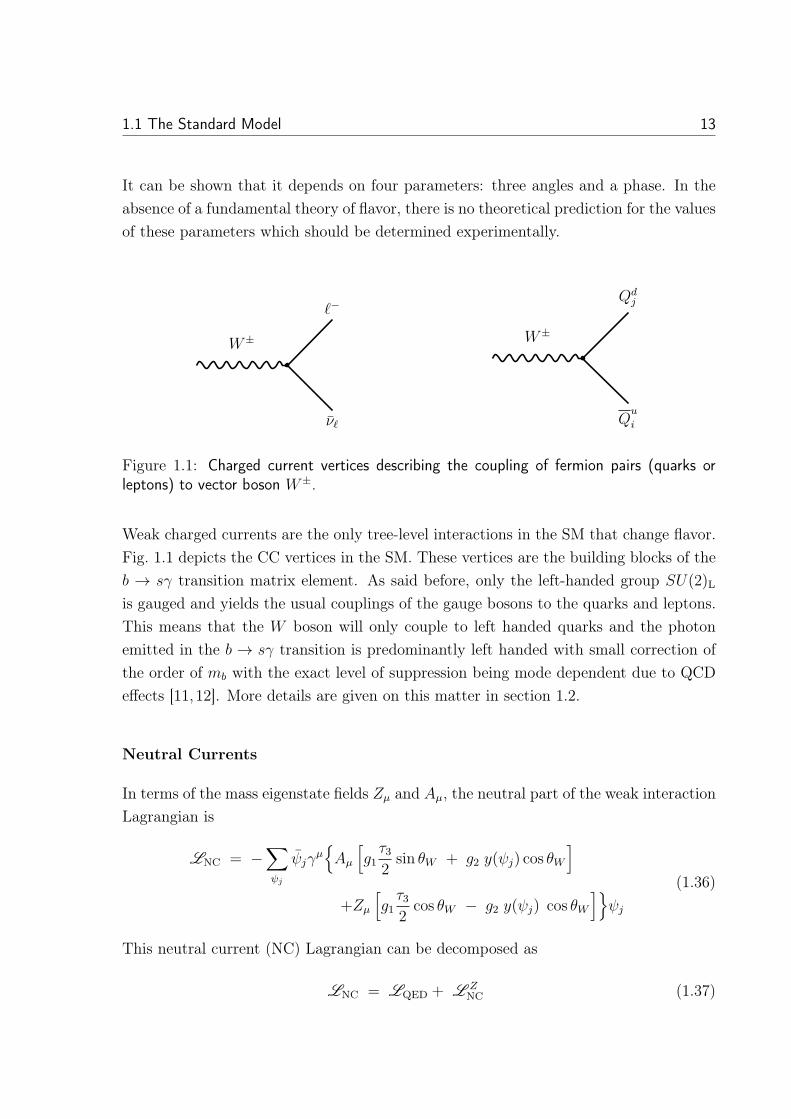
Figure 1.1: Charged current vertices describing the coupling of fermion pairs (quarks orleptons) to vector boson W±.
Weak charged currents are the only tree-level interactions in the SM that change flavor.Fig. 1.1 depicts the CC vertices in the SM. These vertices are the building blocks of theb → sγ transition matrix element. As said before, only the left-handed group SU(2)L
is gauged and yields the usual couplings of the gauge bosons to the quarks and leptons.This means that the W boson will only couple to left handed quarks and the photonemitted in the b → sγ transition is predominantly left handed with small correction ofthe order of mb with the exact level of suppression being mode dependent due to QCDeffects [11, 12]. More details are given on this matter in section 1.2.
Neutral Currents
In terms of the mass eigenstate fields Zμ and Aμ, the neutral part of the weak interactionLagrangian is
LNC = −∑ψj
ψjγμ{Aμ
[g1τ32sin θW + g2 y(ψj) cos θW
]+Zμ
[g1τ32cos θW − g2 y(ψj) cos θW
]}ψj
(1.36)
This neutral current (NC) Lagrangian can be decomposed as
LNC = LQED + L ZNC (1.37)
14 The Electroweak interaction
where LQED is the usual QED Lagrangian, and
L ZNC = − e
2 sin θW cos θWJμZ Zμ (1.38)
which contains the interaction of the boson with the neutral fermionic current JμZ . Equiv-
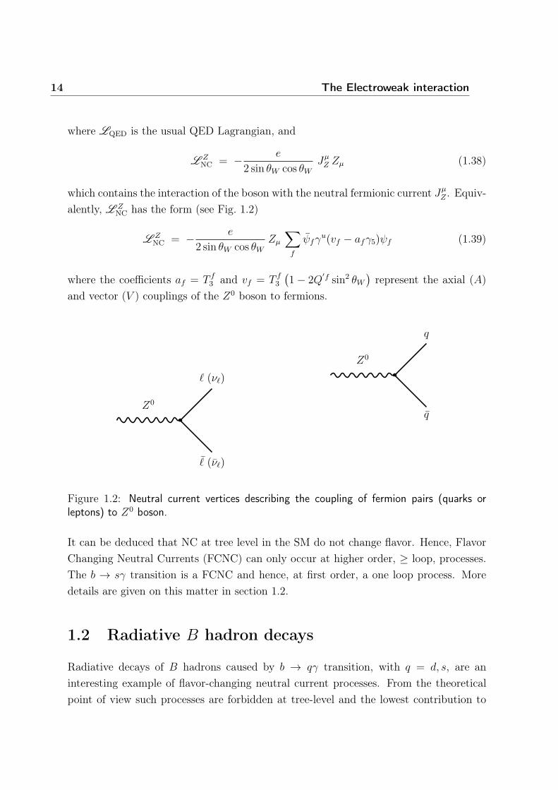
alently, L ZNC has the form (see Fig. 1.2)
L ZNC = − e
2 sin θW cos θWZμ
∑f
ψfγu(vf − afγ5)ψf (1.39)
where the coefficients af = T f3 and vf = T f
3
(1− 2Q
′f sin2 θW)
represent the axial (A)and vector (V ) couplings of the Z0 boson to fermions.
Z0
(ν�)
(ν�)
Z0
q
q
Figure 1.2: Neutral current vertices describing the coupling of fermion pairs (quarks orleptons) to Z0 boson.
It can be deduced that NC at tree level in the SM do not change flavor. Hence, FlavorChanging Neutral Currents (FCNC) can only occur at higher order, ≥ loop, processes.The b → sγ transition is a FCNC and hence, at first order, a one loop process. Moredetails are given on this matter in section 1.2.
1.2 Radiative B hadron decays
Radiative decays of B hadrons caused by b → qγ transition, with q = d, s, are aninteresting example of flavor-changing neutral current processes. From the theoreticalpoint of view such processes are forbidden at tree-level and the lowest contribution to
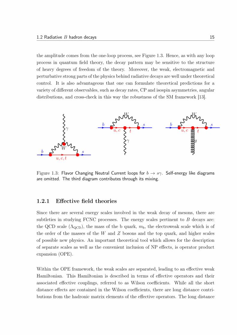
1.2 Radiative B hadron decays 15
the amplitude comes from the one-loop process, see Figure 1.3. Hence, as with any loopprocess in quantum field theory, the decay pattern may be sensitive to the structureof heavy degrees of freedom of the theory. Moreover, the weak, electromagnetic andperturbative strong parts of the physics behind radiative decays are well under theoreticalcontrol. It is also advantageous that one can formulate theoretical predictions for avariety of different observables, such as decay rates, CP and isospin asymmetries, angulardistributions, and cross-check in this way the robustness of the SM framework [13].
b
u, c, t
sW
γb
u, c t
s
W
γ
bu, c t
s
W
g
Figure 1.3: Flavor Changing Neutral Current loops for b → sγ. Self-energy like diagramsare omitted. The third diagram contributes through its mixing.
1.2.1 Effective field theories
Since there are several energy scales involved in the weak decay of mesons, there aresubtleties in studying FCNC processes. The energy scales pertinent to B decays are:the QCD scale (ΛQCD), the mass of the b quark, mb, the electroweak scale which is ofthe order of the masses of the W and Z bosons and the top quark, and higher scalesof possible new physics. An important theoretical tool which allows for the descriptionof separate scales as well as the convenient inclusion of NP effects, is operator productexpansion (OPE).
Within the OPE framework, the weak scales are separated, leading to an effective weakHamiltonian. This Hamiltonian is described in terms of effective operators and theirassociated effective couplings, referred to as Wilson coefficients. While all the shortdistance effects are contained in the Wilson coefficients, there are long distance contri-butions from the hadronic matrix elements of the effective operators. The long distance
16 The Electroweak interaction
effects usually include non-perturbative QCD effects which are the major source of the-oretical uncertainties.
1.2.1.1 Effective Hamiltonian of b → sγ
The effective ΔF = 1 Hamiltonian is given as
Heff =GF√2
∑p=u,c
λ(q)p
[C1Q
p1 + C2Q
p2 +
8∑i=3
CiQi
], (1.40)
where CKM factors are given by λ(q)p = V ∗
pqVpb , and the unitarity relationship hasbeen used. The Wilson coefficients Ci encode physics at large mass scales and hencecarry information about heavy particles - SM as well as NP ones, while matrix ele-ments of hadronic operators Qi are describing long-distance physics dominated by non-perturbative strong interactions. Poor knowledge of these latter factors is the mainsource of uncertainty of theoretical predictions. At leading order the dominant contri-bution comes from the electromagnetic penguin operator
Q7 = −emb(μ)
8π2q σμν [1 + γ5] bFμν (1.41)
Here q = d or s.The factor mb(μ) is the MS mass of the b quark. The Wilson coeffi-cients Ci have been known within the next-to-leading logarithmic approximation (NLL)for over a decade (for a review, see [14]), and have been recently calculated at next-to-next-to-leading logarithmic order (NNLL) in a series of papers [15–18].The standard theoretical procedure used for evaluation of hadronic matrix elements isbased on the QCD factorization idea, augmented by soft-collinear effective theory. Thelatter separates the matrix element of interest into non-perturbative but universal softfunctions (form-factors, decay constants, light-cone distribution amplitudes) and hardscattering kernels calculated as perturbative series in αs. These calculations have beendone in next-to-leading and partly in next-to- next-to-leading order [15]. However thewhole factorization approach makes sense only in the leading order with respect to thesmall parameter ΛQCD/mb and the question of a systematic construction of the 1/mb
expansion remains open. Needless to say, having reliable SM theoretical predictions is anecessary prerequisite for addressing any NP scenario.
1.2 Radiative B hadron decays 17
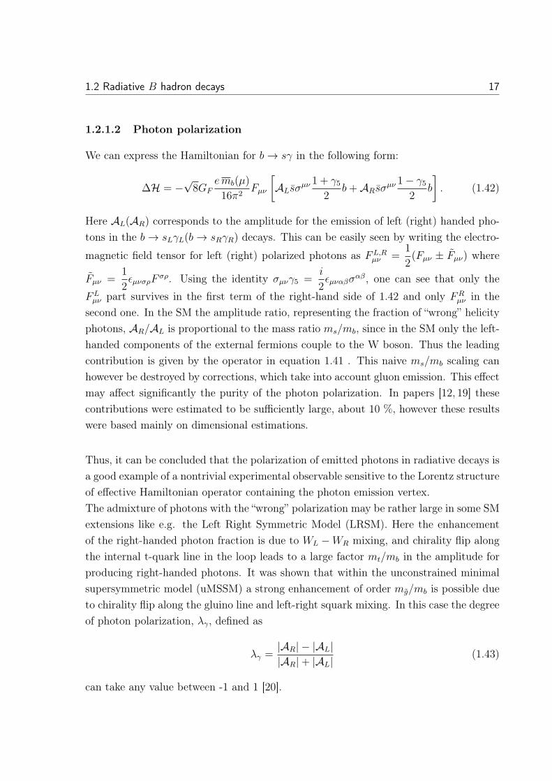
1.2.1.2 Photon polarization
We can express the Hamiltonian for b → sγ in the following form:
ΔH = −√8GF
emb(μ)
16π2Fμν
[ALsσ
μν 1 + γ52
b+ARsσμν 1− γ5
2b
]. (1.42)
Here AL(AR) corresponds to the amplitude for the emission of left (right) handed pho-tons in the b → sLγL(b → sRγR) decays. This can be easily seen by writing the electro-
magnetic field tensor for left (right) polarized photons as FL,Rμν =
1
2(Fμν ± Fμν) where
Fμν =1
2εμνσρF
σρ. Using the identity σμνγ5 =i
2εμναβσ
αβ, one can see that only the
FLμν part survives in the first term of the right-hand side of 1.42 and only FR
μν in thesecond one. In the SM the amplitude ratio, representing the fraction of “wrong” helicityphotons, AR/AL is proportional to the mass ratio ms/mb, since in the SM only the left-handed components of the external fermions couple to the W boson. Thus the leadingcontribution is given by the operator in equation 1.41 . This naive ms/mb scaling canhowever be destroyed by corrections, which take into account gluon emission. This effectmay affect significantly the purity of the photon polarization. In papers [12, 19] thesecontributions were estimated to be sufficiently large, about 10 %, however these resultswere based mainly on dimensional estimations.
Thus, it can be concluded that the polarization of emitted photons in radiative decays isa good example of a nontrivial experimental observable sensitive to the Lorentz structureof effective Hamiltonian operator containing the photon emission vertex.The admixture of photons with the “wrong” polarization may be rather large in some SMextensions like e.g. the Left Right Symmetric Model (LRSM). Here the enhancementof the right-handed photon fraction is due to WL −WR mixing, and chirality flip alongthe internal t-quark line in the loop leads to a large factor mt/mb in the amplitude forproducing right-handed photons. It was shown that within the unconstrained minimalsupersymmetric model (uMSSM) a strong enhancement of order mg/mb is possible dueto chirality flip along the gluino line and left-right squark mixing. In this case the degreeof photon polarization, λγ, defined as
λγ =|AR| − |AL||AR|+ |AL| (1.43)
can take any value between -1 and 1 [20].
18 The Electroweak interaction
1.2.2 Experimental status
In this section, the state of the art of the measurement of the photon polarization inradiative penguin transitions in b hadron decays is presented.
Experimental overview
The aim of the experimental study is to measure the ratio of right-to-left photon polar-ization amplitude
|A(B → ΦγR)||A(B → ΦγL)|
where Φ represents some final hadronic state. There is no clear experimental way tomeasure photon polarization directly, but there are several indirect strategies. The firstone is the study of angular distributions of the Φ decay products [21,22]. In this way oneis able to measure only the square of the amplitude ratio. In such a case, the amplitudescorresponding to left-handed and right-handed photons do not interfere since the polar-ization of the photon in the final state can be measured independently. By studying theangular distribution one can extract the photon polarization, in other words the methodmakes use of angular correlations among the decay products in B → [Φ → P1P2P3]γ,where Pi is either a pion or a kaon. Notice that there must be at least three particles inthe final state so as to define a reference plane with which the orientation of the photonis studied. This technique was used for the decay B → Kππγ [21–23] with the sum overintermediate hadronic resonances. The first direct observation of the photon polariza-tion in the b → sγ transition using B → Kππγ is done by LHCb with a significance of5.2σ [23]. The radiative decay mode B → [φ → K+K−]Kγ is considered in [24]. Thismode is rather distinctive with many desirable features from the experimental point ofview: the final state is a photon plus only charged mesons for charged B mesons, thefact that φ is narrow reduces the effects of intermediate resonances interference, etc.However the actual situation is rather involved. The possibility of measuring the photonpolarization in this way depends on a delicate partial-wave interference pattern. Thelatter may be unfavorable and the asymmetry may escape detection [24].
It would be advantageous to measure the absolute value of the amplitude ratio as itis. There are two possible ways to do that. The first one makes use of the fact thatsome photons convert in the detector material into electron-positron pairs. Thus it ispossible to have the interference between the amplitudes corresponding to left- and right-
1.2 Radiative B hadron decays 19
handed photon emission. It can be shown that for these processes the distribution inthe angle θ between the e+e− plane and the plane defined by the final state hadrons(e.g. Kπ resulting from K∗ decay) should be isotropic for purely circular polarization,while the deviations from this isotropy includes the same parameter AR/AL, indicatingthe presence of right-handed photons [25–28]. However multiple scattering does notallow to identify the decay plane for the low invariant mass e+e−pair. This is not thecase for pair creation from virtual photons where one can select pair masses above 30MeV/c2 without losing too much rate. However in this case other diagrams contributewith longitudinal virtual photons. This measurement is discussed in [29]. The branchingratio of the decay B0 → K∗(892)0e+e− has been measured in the dilepton mass rangeof (30-1000) MeV/c2 [30] and found to be
B(B0→ K∗(892)0e+e−)30−1000 MeV/c2 = (3.1 +0.9 +0.2−0.8 −0.3 ± 0.2)× 10−7.
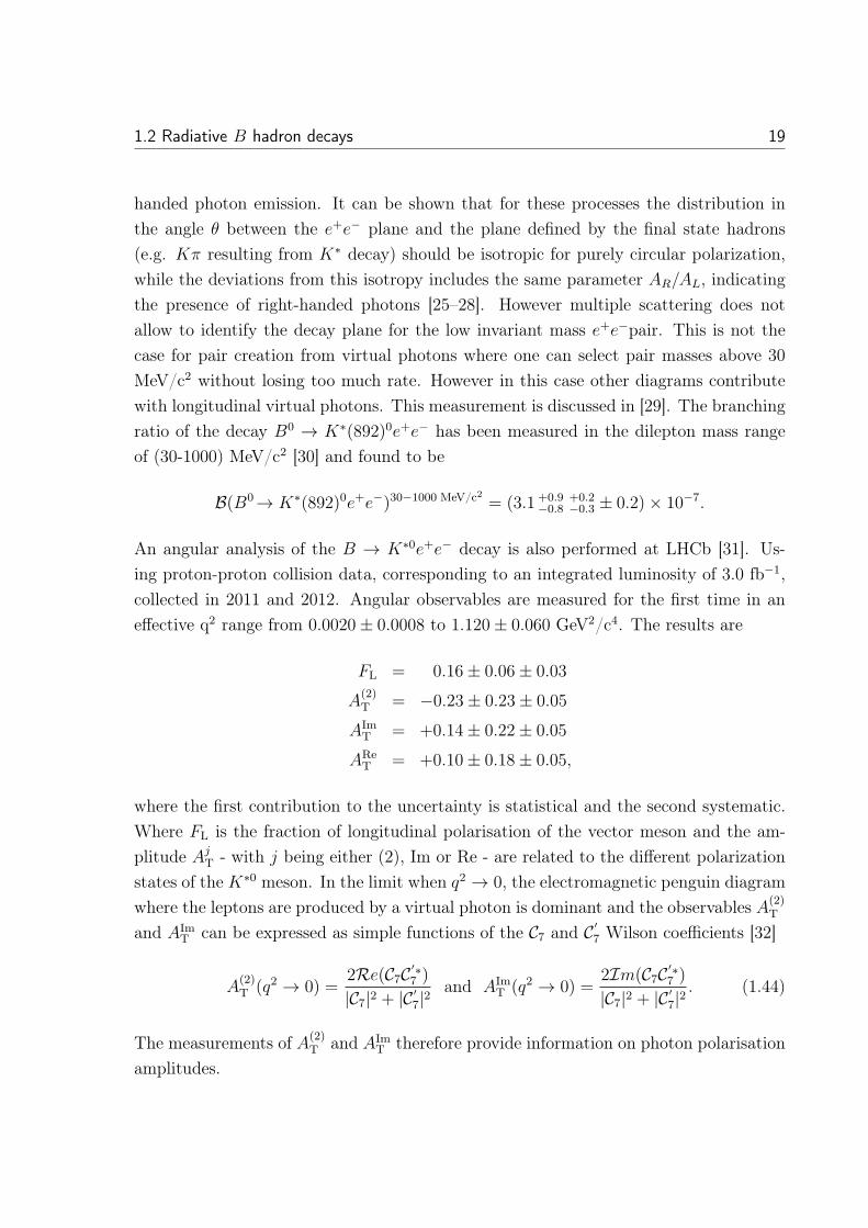
An angular analysis of the B → K∗0e+e− decay is also performed at LHCb [31]. Us-ing proton-proton collision data, corresponding to an integrated luminosity of 3.0 fb−1,collected in 2011 and 2012. Angular observables are measured for the first time in aneffective q2 range from 0.0020± 0.0008 to 1.120± 0.060 GeV2/c4. The results are
FL = 0.16± 0.06± 0.03
A(2)T = −0.23± 0.23± 0.05
AImT = +0.14± 0.22± 0.05
AReT = +0.10± 0.18± 0.05,
where the first contribution to the uncertainty is statistical and the second systematic.Where FL is the fraction of longitudinal polarisation of the vector meson and the am-plitude Aj
T - with j being either (2), Im or Re - are related to the different polarizationstates of the K∗0 meson. In the limit when q2 → 0, the electromagnetic penguin diagramwhere the leptons are produced by a virtual photon is dominant and the observables A(2)
T
and AImT can be expressed as simple functions of the C7 and C ′
7 Wilson coefficients [32]
A(2)T (q2 → 0) =
2Re(C7C ′∗7 )
|C7|2 + |C ′7|2
and AImT (q2 → 0) =
2Im(C7C ′∗7 )
|C7|2 + |C ′7|2
. (1.44)
The measurements of A(2)T and AIm
T therefore provide information on photon polarisationamplitudes.
20 The Electroweak interaction
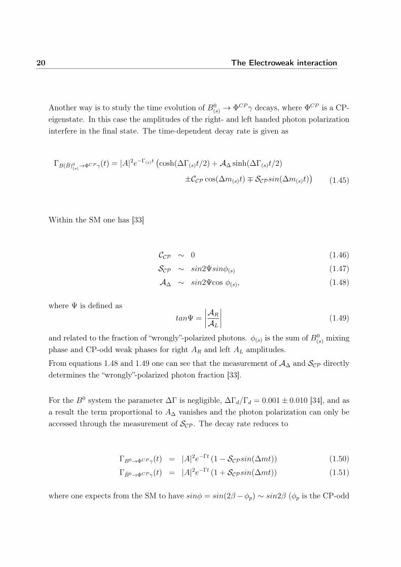
Another way is to study the time evolution of B0(s) → ΦCPγ decays, where ΦCP is a CP-
eigenstate. In this case the amplitudes of the right- and left handed photon polarizationinterfere in the final state. The time-dependent decay rate is given as
ΓB(B)0(s)
→ΦCP γ(t) = |A|2e−Γ(s)t(cosh(ΔΓ(s)t/2) +AΔ sinh(ΔΓ(s)t/2)
±CCP cos(Δm(s)t)∓ SCPsin(Δm(s)t))
(1.45)
Within the SM one has [33]
CCP ∼ 0 (1.46)
SCP ∼ sin2Ψsinφ(s) (1.47)
AΔ ∼ sin2Ψcos φ(s), (1.48)
where Ψ is defined astanΨ =
∣∣∣∣AR
AL
∣∣∣∣ (1.49)
and related to the fraction of “wrongly”-polarized photons. φ(s) is the sum of B0(s) mixing
phase and CP-odd weak phases for right AR and left AL amplitudes.
From equations 1.48 and 1.49 one can see that the measurement of AΔ and SCP directlydetermines the “wrongly”-polarized photon fraction [33].
For the B0 system the parameter ΔΓ is negligible, ΔΓd/Γd = 0.001± 0.010 [34], and asa result the term proportional to AΔ vanishes and the photon polarization can only beaccessed through the measurement of SCP . The decay rate reduces to
ΓB0→ΦCP γ(t) = |A|2e−Γt (1− SCPsin(Δmt)) (1.50)
ΓB0→ΦCP γ(t) = |A|2e−Γt (1 + SCPsin(Δmt)) (1.51)
where one expects from the SM to have sinφ = sin(2β−φp) ∼ sin2β (φp is the CP-odd
1.2 Radiative B hadron decays 21
weak penguin phase) and hence, SCP is given as
SCP = sin2Ψsin2β. (1.52)
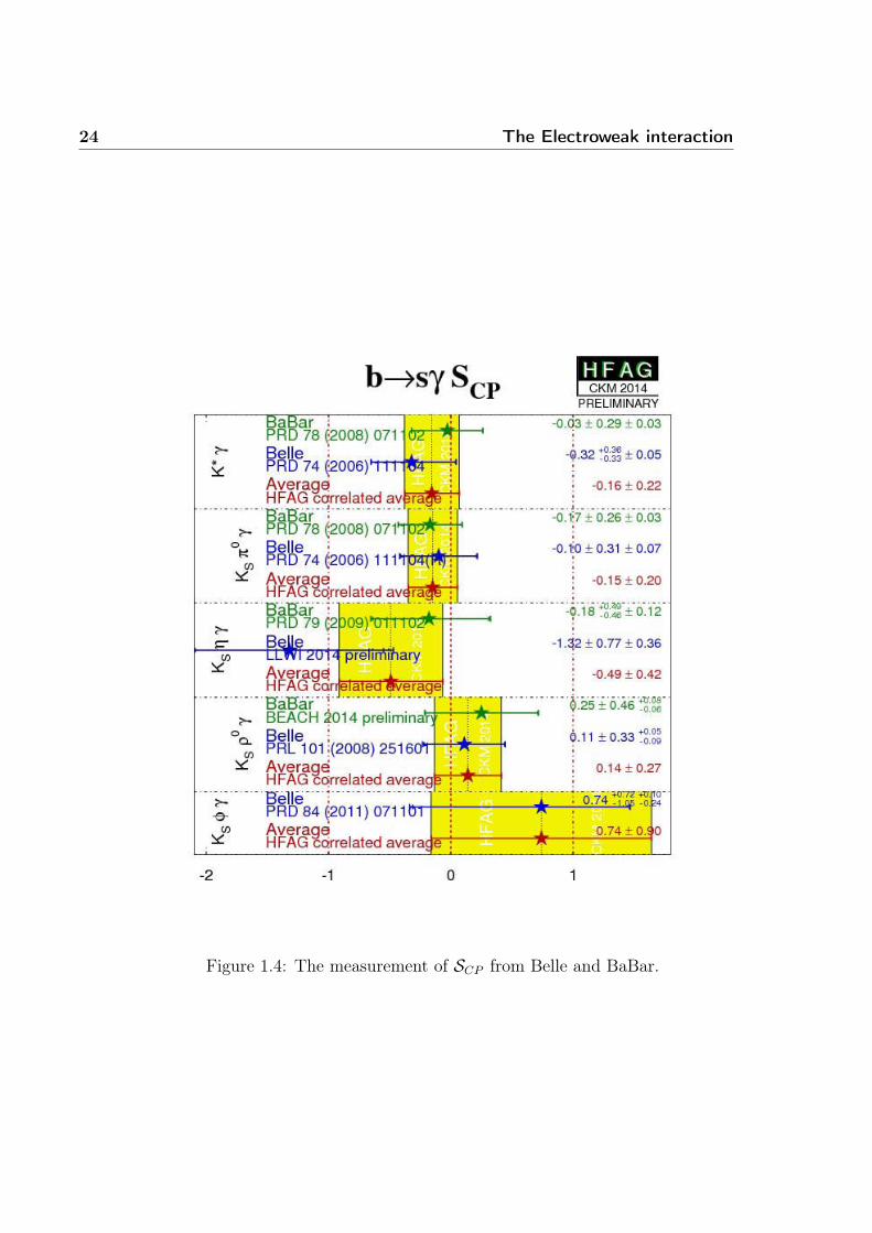
This approach can be accessed from the decay channel B0 → [K∗0 → Ksπ0]γ, it has
been done at BABAR and Belle [35, 36] (figure 1.4) but very challenging at LHCb dueto the presence of only neutrals in the final state.An inclusive B0 → KSπ
0γ analysis has been performed by Belle using the invariantmass range up to 1.8 GeV/c2. Belle also gives results for the K∗(892) region: 0.8GeV/c2 to 1.0 GeV/c2. BaBar has measured the CP-violating asymmetries separatelywithin and outside the K∗(892) mass range: 0.8 GeV/c2 to 1.0 GeV/c2 is again used forB0 → K∗0(892)γ candidates, while events with invariant masses in the range 1.1 GeV/c2
to 1.8 GeV/c2 are used in the B0 → KSπ0γ analysis [35]. Figure 1.4 summarizes the
results of BaBar and Belle concerning the measurement of SCP .
For the B0s system the parameter ΔΓs is not negligible, providing a non- zero sensitivity
to AΔ. In the SM φs is expected to be small, sinφs = sin(2βs − φp) ≈ 0, thus the termwith S vanishes:
ΓB0(s)
→ΦCP γ(t) = ΓB0(s)
→ΦCP γ(t) = |A|2e−Γ(s)t(cosh(ΔΓ(s)t/2) +AΔ sinh(ΔΓ(s)t/2)
)(1.53)
and finally one has
AB0
sΔ ∼ sin2Ψ, (1.54)
thus opening the possibility for the direct measurement of the photon polarization pa-rameter sin2ψ [37]. It is worth to stress here that contributions from SCP and CCP vanishwhen considering the inclusive ΓBs + ΓBs
assuming the Bs/Bs production asymmetryvanish. The analysis of B0
s → φγ addressed in this thesis is based on this approach.
Alternatively, one can study baryon decays Λb → Λ0γ → pπγ (or Λb → Λ∗γ → pKγ )and measure the photon polarization via the forward-backward asymmetry of the protonwith respect to the Λb in the Λ0 rest frame for polarized Λb, (see [38–41] for details andreferences therein). The main problem of these two methods is the absence of interferencebetween the amplitudes corresponding to left- and right- handed photon emission sincethey correspond to different and distinguishable final states. Correspondingly they are
22 The Electroweak interaction
sensitive only to the square of the amplitude ratio in the form of photon polarization λγ
(equation 1.43). Moreover, the measurement of the photon polarization with radiativebaryon decays have proved experimentally difficult due to the small polarisation of Λ0
b
baryons produced at the LHC [42]. The polarization of Λ0b is required to be non-zero for
the measurement of the photon polarization.
Radiative b hadron decays provide the potential for significant future improvement in theknowledge of right-handed contributions to the b → sγ amplitude. To achieve this it isnecessary to use all of the methods most sensitive to the photon polarisation, since theyprovide complementary information [43]. These methods include time-dependent asym-metries in B0 → Ksπ
0γ and B0s → φγ decays, up-down asymmetries in B+ → K+π+π−γ
decays, and angular asymmetries in B0 → K∗0e+e− decays, baryon radiative decaysΛb → Λ∗γ and many other decays. Improved searches for CP violation in both inclusiveand exclusive processes are important. There are excellent prospects for progress in mostof these areas at both LHCb, including its upgrade [44], and Belle II.
1.2.3 Radiative B decays at LHCb
LHCb capability of performing analysis of radiative decays has been demonstratedthrough several measurements [23, 30, 31, 45]. The presence of the photon, which isreconstructed in the calorimeter, in the final state makes the reconstruction of the decayexperimentally challenging. The resolution of the different decay variables is driven bythe resolution of the calorimeter. Moreover, the presence of a neutral particle in thedecay’s final state engenders a high level of background for the reconstructed radiativedecay.
In addition to the analysis already cited in the previous section, LHCb has publishedseveral results on radiative B decays. First, the measurement of the ratio of branchingratios B(B0
s → φγ)/B(B0→ K∗(892)0γ) [45] has been performed with the data collectedby LHCb in 2011
B(B0s → φγ)/B(B0→ K∗(892)0γ) = 1.23± 0.06(stat.)± 0.04(syst.)± 0.10 fs/fd
from which the branching ratio of B0s → φγ can be extracted using, back when the paper
was published, the 2010 HFAG [34] value for the branching ratio of B0→ K∗(892)0γ
B(B0s → φγ) = (3.5± 0.4)× 10−5.
1.2 Radiative B hadron decays 23
With the same data set, the direct CP asymmetry of B0→ K∗(892)0γ is measured [45]
ACP (B0→ K∗(892)0γ) = (0.8± 1.7(stat.)± 0.9(syst.))%.
LHCb has collected during the 2011-2012 run period the largest sample of B0s → φγ
events. The analysis performed in this thesis is based on this sample that is selectedfollowing what has been done in [45].
In Run II, the LHC will operate at a center of mass energy of√s = 14 TeV during the
first year. With this increase of energy, the integrated luminosity collected by LHCbwill be twice what LHCb collected during the Run I.The huge amount of statistics will give way to new measurements in the b → dγ sectoras well as baryon radiative decays, Λb → Λ∗γ and many other decays [41].
24 The Electroweak interaction
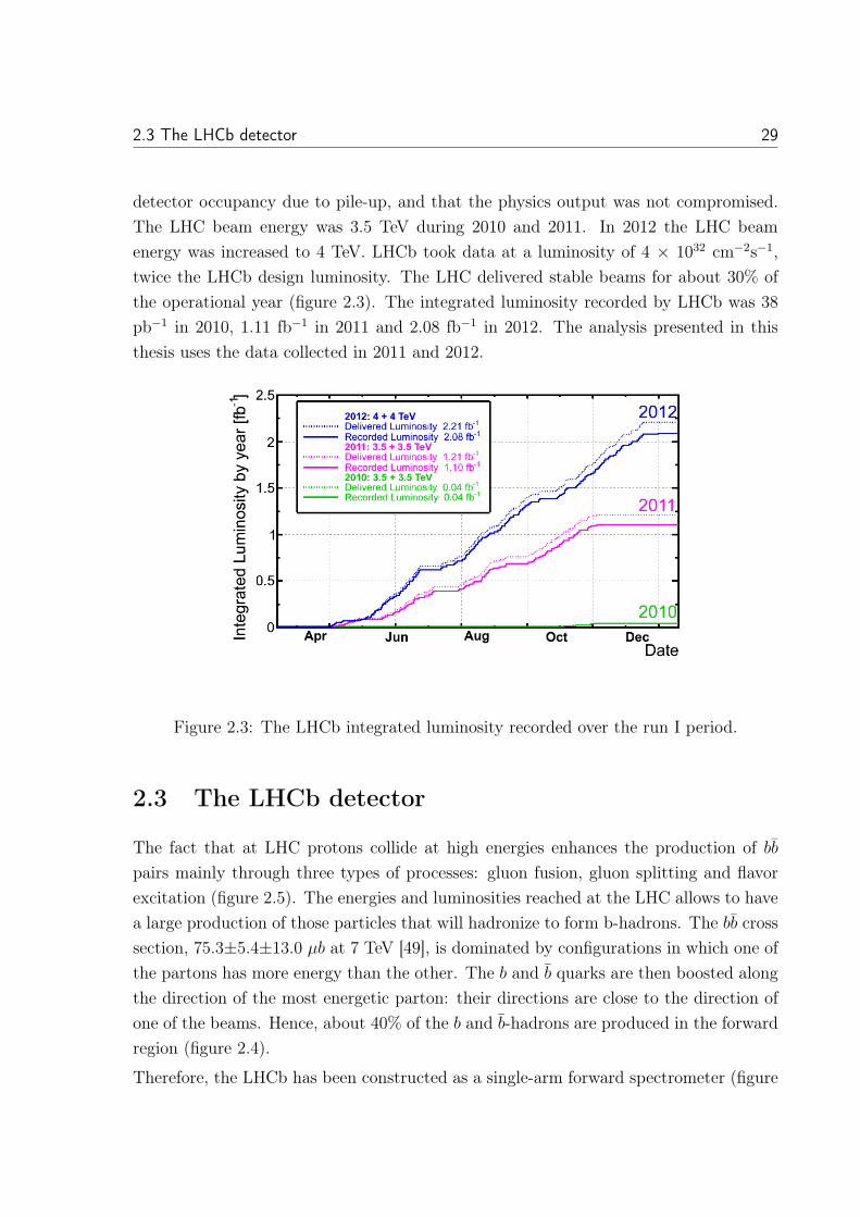
Figure 1.4: The measurement of SCP from Belle and BaBar.

Chapter 2
The LHCb
Contents2.1 The LHC . . . . . . . . . . . . . . . . . . . . . . . . . . . . . . 26
2.2 Data taking periods and operating conditions . . . . . . . . 28
2.3 The LHCb detector . . . . . . . . . . . . . . . . . . . . . . . . 29
2.3.1 Vertex reconstruction: The VELO . . . . . . . . . . . . . . . . 33
2.3.2 Momentum measurement: The dipole magnet . . . . . . . . . . 34
2.3.3 Track reconstruction: Silicon Trackers and Outer Trackers . . . 35
2.3.4 Ring imaging Cherenkov detectors . . . . . . . . . . . . . . . . 37
2.3.5 The Calorimeters . . . . . . . . . . . . . . . . . . . . . . . . . . 38
2.3.6 The Muon detector . . . . . . . . . . . . . . . . . . . . . . . . . 44
2.3.7 Particle Identification . . . . . . . . . . . . . . . . . . . . . . . 46
2.4 The LHCb trigger system . . . . . . . . . . . . . . . . . . . . 48
2.4.1 The Level-0 trigger . . . . . . . . . . . . . . . . . . . . . . . . . 49
2.4.2 The High Level Trigger . . . . . . . . . . . . . . . . . . . . . . 51
2.5 The LHCb luminosity measurements . . . . . . . . . . . . . . 52
2.6 The LHCb software . . . . . . . . . . . . . . . . . . . . . . . . 53
2.7 Data flow in LHCb . . . . . . . . . . . . . . . . . . . . . . . . 54
25
26 The LHCb
The LHCb experiment is one of four main experiments collecting data at theLarge Hadron Collider accelerator at CERN. LHCb has a wide physics program coveringmany important aspects of Heavy Flavor, Electroweak and QCD physics. It is mainlyspecialized in flavor physics and is collecting data that is used to perform measurementsof the parameters of CP violation in the interactions of b-hadrons. Such studies can helpto explain the Matter-Antimatter asymmetry of the Universe. The detector is also ableto collect data to perform measurements of production cross sections and electroweakphysics in the forward region. Its key measurements, one of which is the measurementof the photon polarization, are described in a roadmap document [46]. Many of these keymeasurement have already been performed. In this chapter, the LHCb experiment will bedescribed detailing how the decay’s vertex is reconstructed, how the momentum/energy ofthe decay’s products and their tracks are measured and how these products are identified;the LHCb sub-detectors will be explained as well as the hardware and software triggers.Finally, the LHCb performance during the 2011-2012 run period will be discussed.
2.1 The LHC
The biggest particle accelerator ever built is the Large Hadron Collider (LHC). It con-sists of a circular tunnel of 27 km, located underground at the french-swiss border [47].This machine has been designed for proton-proton (pp) collisions. Two beams of protonstravel inside the tunnel in opposite directions inside two different pipes. Each beam con-sists in sets of grouped protons called bunches, each one containing 1.15× 10¹¹ protonson average. There are more than 2808 bunches in each beam at full intensity. Thecollisions occur in determined places around the rings, called interaction points, wherethe two bunches cross each other. This is where the detectors are located. There arefour principal experiments at the LHC. The ATLAS and CMS detectors [60, 61] aregeneral purpose experiments, mainly designed to search for the Higgs boson and fordirect evidence of physics beyond the Standard Model. The ALICE experiment [62]is dedicated to the reconstruction of heavy ions collisions in order to study the forma-tion of the quark-gluon plasma. Finally the LHCb experiment, in which this work tookplace, is designed for precision measurements on beauty and charm physics, speciallythe study of CP violation in this sector [63]. To reach those challenging physics goals,it is necessary to accumulate a big amount of data at collision energies never achieved
2.1 The LHC 27
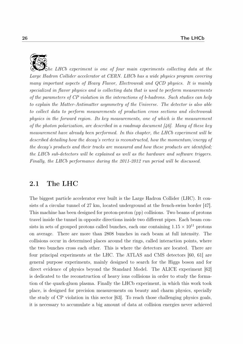
before. In 2010-2011 LHC ran at a center of mass energy of 7 TeV. The center of massenergy was increased to 8 TeV in 2012. The protons are injected from the Super ProtonSynchrotron (SPS) at the energy of 450 GeV. Inside the LHC, protons are acceleratedto reach their final energy. A general view of the LHC complex can be found in figure 2.1.
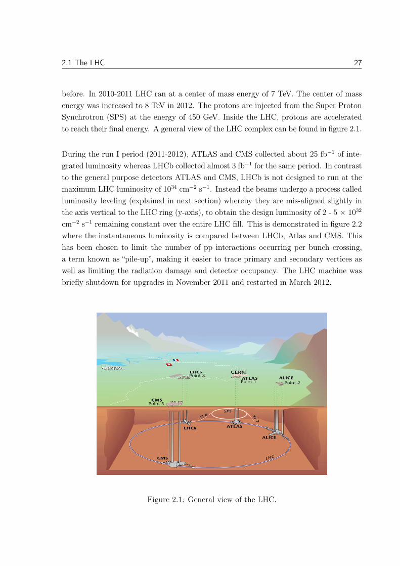
During the run I period (2011-2012), ATLAS and CMS collected about 25 fb−1 of inte-grated luminosity whereas LHCb collected almost 3 fb−1 for the same period. In contrastto the general purpose detectors ATLAS and CMS, LHCb is not designed to run at themaximum LHC luminosity of 1034 cm−2 s−1. Instead the beams undergo a process calledluminosity leveling (explained in next section) whereby they are mis-aligned slightly inthe axis vertical to the LHC ring (y-axis), to obtain the design luminosity of 2 - 5 × 1032
cm−2 s−1 remaining constant over the entire LHC fill. This is demonstrated in figure 2.2where the instantaneous luminosity is compared between LHCb, Atlas and CMS. Thishas been chosen to limit the number of pp interactions occurring per bunch crossing,a term known as “pile-up”, making it easier to trace primary and secondary vertices aswell as limiting the radiation damage and detector occupancy. The LHC machine wasbriefly shutdown for upgrades in November 2011 and restarted in March 2012.
Figure 2.1: General view of the LHC.
28 The LHCb
Figure 2.2: Development of the instantaneous luminosity for ATLAS, CMS and LHCbduring LHC fill 2651. After ramping to the desired value of 4×1032cm2s−1 for LHCb, theluminosity is kept stable in a range of 5% for about 15 hours by adjusting the transversalbeam overlap.The difference in luminosity towards the end of the fill between ATLAS,CMS and LHCb is due to the difference in the final focusing at the collision points.
2.2 Data taking periods and operating conditions
At the end of 2009, LHCb recorded its first pp collisions at the injection energy of theLHC,
√s = 0.9TeV. These data have been used to finalise the commissioning of the
sub-detector systems and the reconstruction software, and to perform a first alignmentand calibration of the tracking, calorimeter and particle identification (PID) systems.In this period, the VErtex LOcator (VELO, presented in section 2.3.1) was left in theopen position, due to the larger aperture required at lower beam energies. During 2010the operating conditions changed rapidly due to the ramp-up of the LHC luminosity. Acritical parameter for LHCb performance is the pile-up, defined as the average numberof visible interactions per beam-beam crossing [48]. While the highest luminosity in 2010was already 75% of the LHCb design luminosity, the pile-up was much larger than thedesign value due to the low number of bunches in the machine. It was demonstrated thatthe trigger and reconstruction work efficiently under such harsh conditions with increased
2.3 The LHCb detector 29
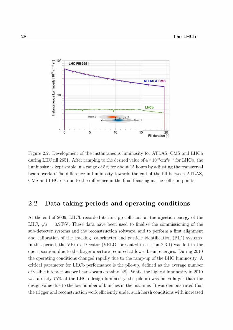
detector occupancy due to pile-up, and that the physics output was not compromised.The LHC beam energy was 3.5 TeV during 2010 and 2011. In 2012 the LHC beamenergy was increased to 4 TeV. LHCb took data at a luminosity of 4 × 1032 cm−2s−1,twice the LHCb design luminosity. The LHC delivered stable beams for about 30% ofthe operational year (figure 2.3). The integrated luminosity recorded by LHCb was 38pb−1 in 2010, 1.11 fb−1 in 2011 and 2.08 fb−1 in 2012. The analysis presented in thisthesis uses the data collected in 2011 and 2012.
Figure 2.3: The LHCb integrated luminosity recorded over the run I period.
2.3 The LHCb detector
The fact that at LHC protons collide at high energies enhances the production of bb
pairs mainly through three types of processes: gluon fusion, gluon splitting and flavorexcitation (figure 2.5). The energies and luminosities reached at the LHC allows to havea large production of those particles that will hadronize to form b-hadrons. The bb crosssection, 75.3±5.4±13.0 μb at 7 TeV [49], is dominated by configurations in which one ofthe partons has more energy than the other. The b and b quarks are then boosted alongthe direction of the most energetic parton: their directions are close to the direction ofone of the beams. Hence, about 40% of the b and b-hadrons are produced in the forwardregion (figure 2.4).
Therefore, the LHCb has been constructed as a single-arm forward spectrometer (figure

30 The LHCb
Figure 2.4: Polar angles of the b and b-hadrons produced at the LHC, as obtained froma PYTHIA simulation.
2.7) with a angular acceptance ranging from 10 to 300 mrad in the magnet bendingplane (plane horizontal with the LHC ring) and to 250 mrad in the plane vertical to theLHC ring (figure 2.6).
The nominal interaction point defines the center of the coordinate system. The x, y andz axes form a right handed orthogonal system: the (x, z) plane contains the acceleratorwith the x axis being orthogonal to the beam direction and the z axis being parallel tothe beam direction. They y axis is orthogonal to the (x, z) plane.
Figure 2.5: Feynman diagrams of processes related to bb production at the LHC, gluonfusion (left), gluon splitting (middle) and flavor excitation (right).
2.3 The LHCb detector 31
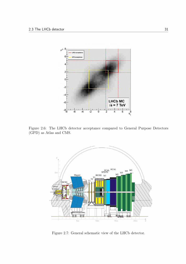
Figure 2.6: The LHCb detector acceptance compared to General Purpose Detectors(GPD) as Atlas and CMS.
Figure 2.7: General schematic view of the LHCb detector.
32 The LHCb
The accelerator increases its delivered luminosity so as to accumulate a large statistics.This increases the average number of proton-proton collisions per bunch crossing. In-creasing the number of proton-proton collisions has a cost, it increases the multiplicityof particles in the event and makes the event reconstruction more difficult. This is morecritical in the forward region where the occupancy is higher. Another important point isthat for an event with multiple proton-proton interactions there could be an ambiguityin associating a b-hadron to the right production vertex as the b-hadrons reconstructedin the experiment are mainly produced in the forward direction. At LHCb, the beam isless focused and the method of luminosity leveling by beam separation is used insuringa stable instantaneous luminosity. Figure 2.2 shows the concept of luminosity levelingwhich consists in moving the proton beams relative to each other modifying the effectivecrossing area. The fact that the instantaneous luminosity is stable at LHCb means thatthere is a stable average number of visible interactions per bunch crossing over a fillduration.There are three stages in which b-hadrons decays are identified at LHCb. First, vertexreconstruction is essential since the b-hadron has a relatively long lifetime, about 1.5 ps(except for the Bc which lifetime is about 0.5 ps and the B∗ which is strongly decaying),which means that the proton-proton interaction vertex, denoted primary vertex (PV), isdifferent than the b-hadron decay vertex, denoted secondary vertex (SV). The separationbetween those two vertices is important so as to separate between tracks coming fromthe PV and others coming from the SV as well as to check that the latter points to thesame decay point; this is assured by the vertex locator, denoted as VELO. Then comesthe energy/momentum measurements which is the key point to reconstruct the mass ofthe b-hadron and the mass of any intermediate resonance, the better the mass resolutionwe can get the better is the background rejection that we can achieve. Charged particlemomentum is measured by the tracking system whereas the calorimeter is responsiblefor the measurement of photon and neutral pion energy. The final criteria to have a wellreconstructed b-hadron decay is to have a good particle identification. Pions, kaons andprotons are identified by two ring imaging Cherenkov; electrons, photons and neutralpions are identified in the calorimeter and the muon chambers identify muons.
2.3 The LHCb detector 33
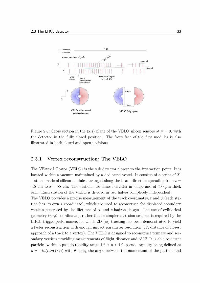
Figure 2.8: Cross section in the (x,z) plane of the VELO silicon sensors at y = 0, withthe detector in the fully closed position. The front face of the first modules is alsoillustrated in both closed and open positions.
2.3.1 Vertex reconstruction: The VELO
The VErtex LOcator (VELO) is the sub detector closest to the interaction point. It islocated within a vacuum maintained by a dedicated vessel. It consists of a series of 21stations made of silicon modules arranged along the beam direction spreading from z =-18 cm to z = 88 cm. The stations are almost circular in shape and of 300 μm thickeach. Each station of the VELO is divided in two halves completely independent.The VELO provides a precise measurement of the track coordinates, r and φ (each sta-tion has its own z coordinate), which are used to reconstruct the displaced secondaryvertices generated by the lifetimes of b- and c-hadron decays. The use of cylindricalgeometry (z,r,φ coordinates), rather than a simpler cartesian scheme, is required by theLHCb trigger performance, for which 2D (rz) tracking has been demonstrated to yielda faster reconstruction with enough impact parameter resolution (IP, distance of closestapproach of a track to a vertex). The VELO is designed to reconstruct primary and sec-ondary vertices providing measurements of flight distance and of IP. It is able to detectparticles within a pseudo rapidity range 1.6 < η < 4.9, pseudo rapidity being defined asη = −ln(tan(θ/2)) with θ being the angle between the momentum of the particle and
34 The LHCb
the beam axis, and emerging from interactions in the range |z| < 10.6 cm, it has a singlehit precision of ∼ 4 μm requiring high precision on its alignment.
Each half station is composed of two types of sensors: the r-sensors and the φ-sensors.The r-sensors consist in semi-circles centred on the beam axis. This allows the deter-mination of the r coordinate which is the distance to the beam axis. The φ-sensors aredivided radially to determine the φ-coordinate defined as the angle with respect to thex axis in the (x, y) plane. The z coordinate is obtained from the position of the station.The sensitive part of VELO sensors starts at a radius of about 8 mm, which is thesmallest possible for safety reasons. During injection, however, the aperture required bythe LHC machine increases, so the VELO is retracted up to a distance of 3 cm as can beseen in figure 2.8. The VELO may be closed only after stabilization of the beams. It canbe fully operated in both positions, opened or closed. Two additional stations, calledpile-up stations, constituted by r-sensor modules, are placed upstream of the interactionpoint to allow a fast determination of the number of primary vertices that can be usedin the first trigger level (L0). At LHCb, to define a track, hits are required in at leastthree modules. The spatial resolution on the primary vertex depends on the number oftracks, but on average it is found to be about 42 μm on the z-axis direction and about10 μm in the (r, φ) plane.
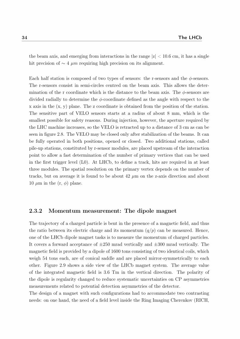
2.3.2 Momentum measurement: The dipole magnet
The trajectory of a charged particle is bent in the presence of a magnetic field, and thusthe ratio between its electric charge and its momentum (q/p) can be measured. Hence,one of the LHCb dipole magnet tasks is to measure the momentum of charged particles.It covers a forward acceptance of ±250 mrad vertically and ±300 mrad vertically. Themagnetic field is provided by a dipole of 1600 tons consisting of two identical coils, whichweigh 54 tons each, are of conical saddle and are placed mirror-symmetrically to eachother. Figure 2.9 shows a side view of the LHCb magnet system. The average valueof the integrated magnetic field is 3.6 Tm in the vertical direction. The polarity ofthe dipole is regularity changed to reduce systematic uncertainties on CP asymmetriesmeasurements related to potential detection asymmetries of the detector.The design of a magnet with such configurations had to accommodate two contrastingneeds: on one hand, the need of a field level inside the Ring Imaging Cherenkov (RICH,
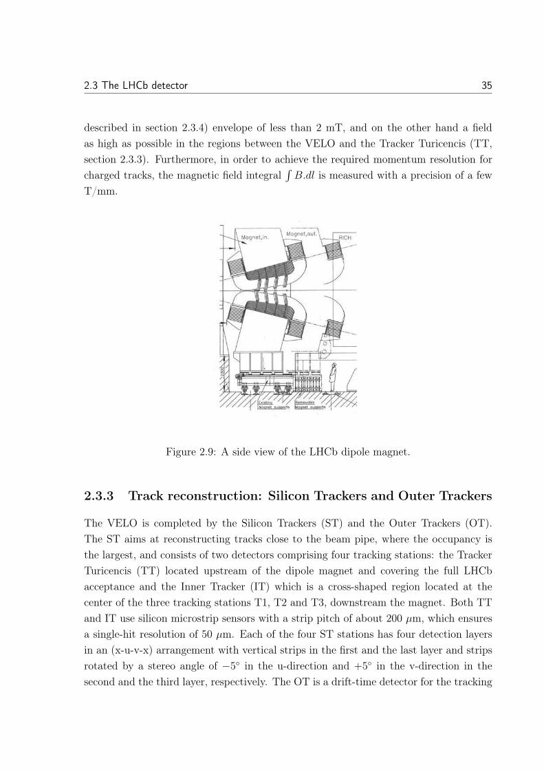
2.3 The LHCb detector 35
described in section 2.3.4) envelope of less than 2 mT, and on the other hand a fieldas high as possible in the regions between the VELO and the Tracker Turicencis (TT,section 2.3.3). Furthermore, in order to achieve the required momentum resolution forcharged tracks, the magnetic field integral
∫B.dl is measured with a precision of a few
T/mm.
Figure 2.9: A side view of the LHCb dipole magnet.
2.3.3 Track reconstruction: Silicon Trackers and Outer Trackers
The VELO is completed by the Silicon Trackers (ST) and the Outer Trackers (OT).The ST aims at reconstructing tracks close to the beam pipe, where the occupancy isthe largest, and consists of two detectors comprising four tracking stations: the TrackerTuricencis (TT) located upstream of the dipole magnet and covering the full LHCbacceptance and the Inner Tracker (IT) which is a cross-shaped region located at thecenter of the three tracking stations T1, T2 and T3, downstream the magnet. Both TTand IT use silicon microstrip sensors with a strip pitch of about 200 μm, which ensuresa single-hit resolution of 50 μm. Each of the four ST stations has four detection layersin an (x-u-v-x) arrangement with vertical strips in the first and the last layer and stripsrotated by a stereo angle of −5◦ in the u-direction and +5◦ in the v-direction in thesecond and the third layer, respectively. The OT is a drift-time detector for the tracking
36 The LHCb
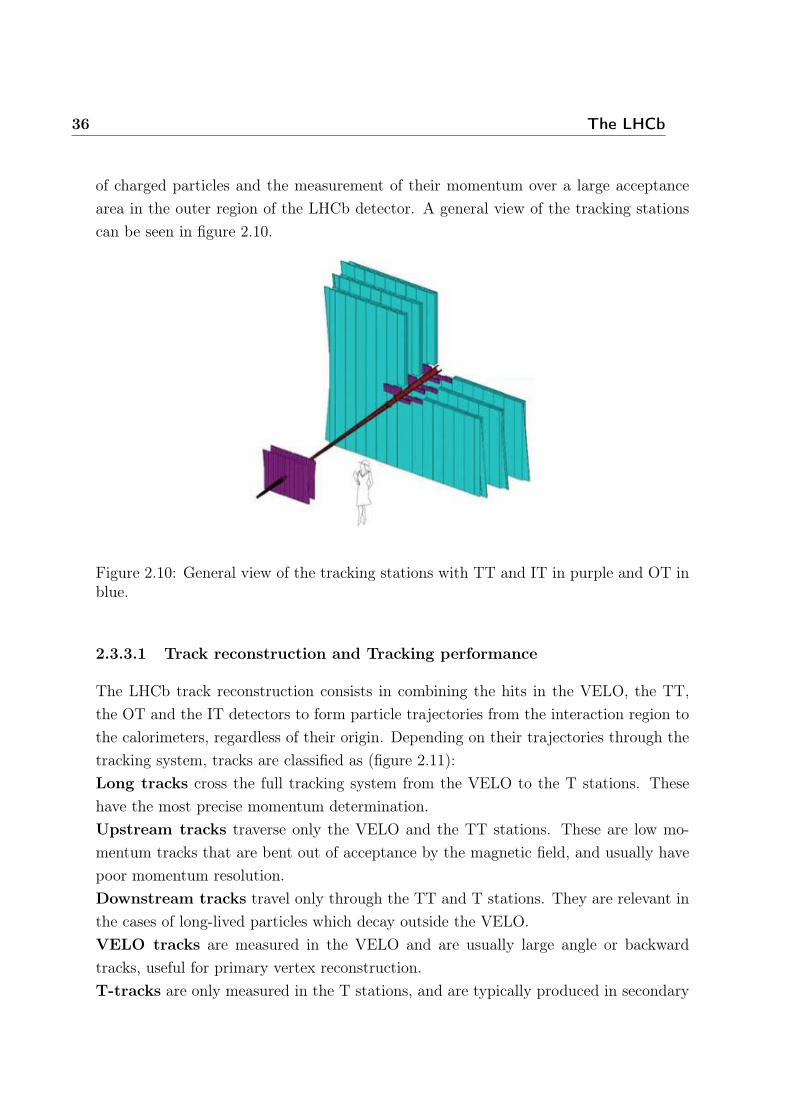
of charged particles and the measurement of their momentum over a large acceptancearea in the outer region of the LHCb detector. A general view of the tracking stationscan be seen in figure 2.10.
Figure 2.10: General view of the tracking stations with TT and IT in purple and OT inblue.
2.3.3.1 Track reconstruction and Tracking performance
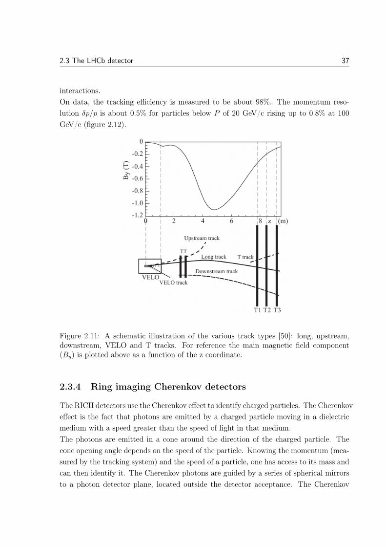
The LHCb track reconstruction consists in combining the hits in the VELO, the TT,the OT and the IT detectors to form particle trajectories from the interaction region tothe calorimeters, regardless of their origin. Depending on their trajectories through thetracking system, tracks are classified as (figure 2.11):Long tracks cross the full tracking system from the VELO to the T stations. Thesehave the most precise momentum determination.Upstream tracks traverse only the VELO and the TT stations. These are low mo-mentum tracks that are bent out of acceptance by the magnetic field, and usually havepoor momentum resolution.Downstream tracks travel only through the TT and T stations. They are relevant inthe cases of long-lived particles which decay outside the VELO.VELO tracks are measured in the VELO and are usually large angle or backwardtracks, useful for primary vertex reconstruction.T-tracks are only measured in the T stations, and are typically produced in secondary
2.3 The LHCb detector 37
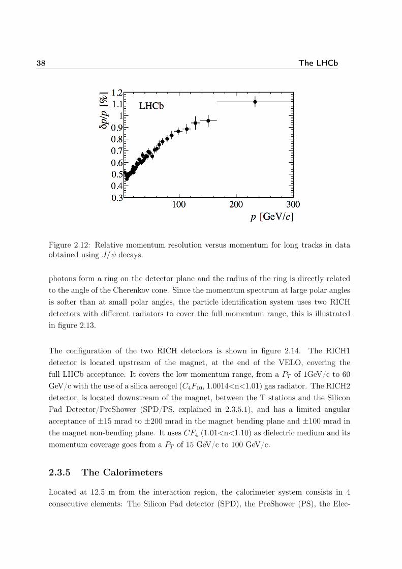
interactions.On data, the tracking efficiency is measured to be about 98%. The momentum reso-lution δp/p is about 0.5% for particles below P of 20 GeV/c rising up to 0.8% at 100GeV/c (figure 2.12).
Figure 2.11: A schematic illustration of the various track types [50]: long, upstream,downstream, VELO and T tracks. For reference the main magnetic field component(By) is plotted above as a function of the z coordinate.
2.3.4 Ring imaging Cherenkov detectors
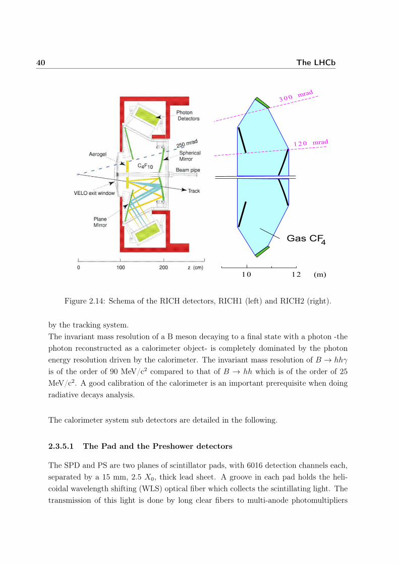
The RICH detectors use the Cherenkov effect to identify charged particles. The Cherenkoveffect is the fact that photons are emitted by a charged particle moving in a dielectricmedium with a speed greater than the speed of light in that medium.The photons are emitted in a cone around the direction of the charged particle. Thecone opening angle depends on the speed of the particle. Knowing the momentum (mea-sured by the tracking system) and the speed of a particle, one has access to its mass andcan then identify it. The Cherenkov photons are guided by a series of spherical mirrorsto a photon detector plane, located outside the detector acceptance. The Cherenkov
38 The LHCb
Figure 2.12: Relative momentum resolution versus momentum for long tracks in dataobtained using J/ψ decays.
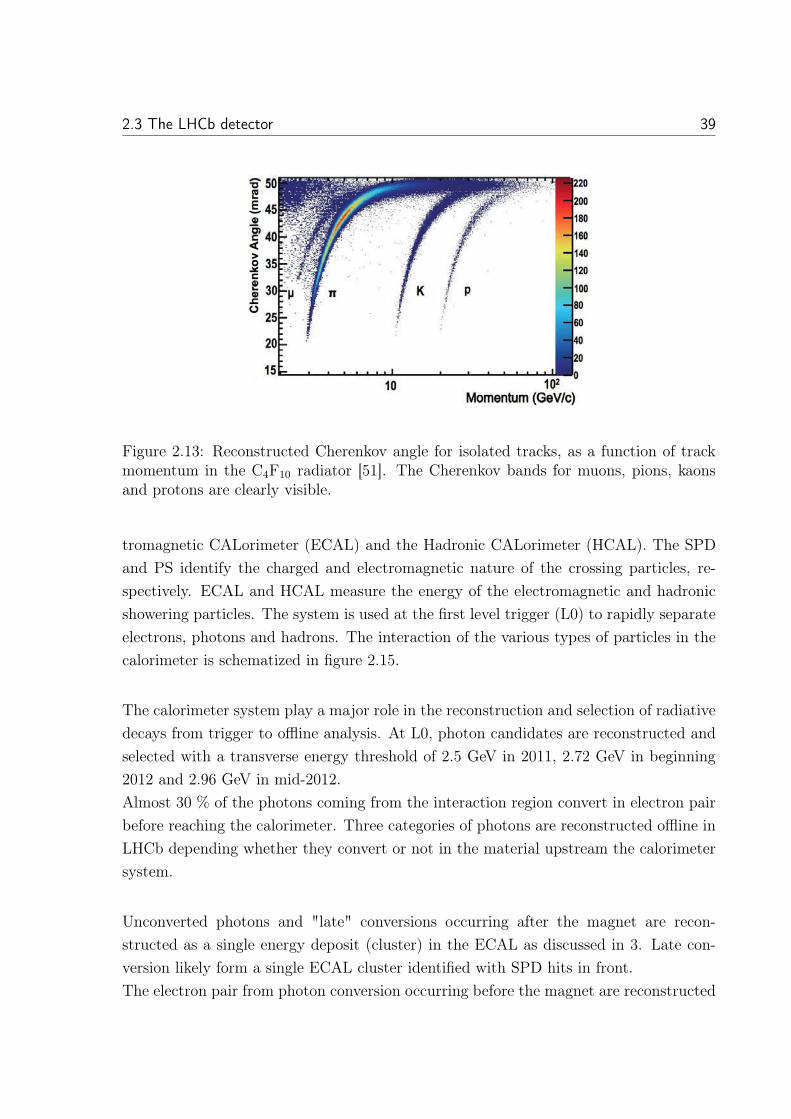
photons form a ring on the detector plane and the radius of the ring is directly relatedto the angle of the Cherenkov cone. Since the momentum spectrum at large polar anglesis softer than at small polar angles, the particle identification system uses two RICHdetectors with different radiators to cover the full momentum range, this is illustratedin figure 2.13.
The configuration of the two RICH detectors is shown in figure 2.14. The RICH1detector is located upstream of the magnet, at the end of the VELO, covering thefull LHCb acceptance. It covers the low momentum range, from a PT of 1GeV/c to 60GeV/c with the use of a silica aereogel (C4F10, 1.0014<n<1.01) gas radiator. The RICH2detector, is located downstream of the magnet, between the T stations and the SiliconPad Detector/PreShower (SPD/PS, explained in 2.3.5.1), and has a limited angularacceptance of ±15 mrad to ±200 mrad in the magnet bending plane and ±100 mrad inthe magnet non-bending plane. It uses CF4 (1.01<n<1.10) as dielectric medium and itsmomentum coverage goes from a PT of 15 GeV/c to 100 GeV/c.
2.3.5 The Calorimeters
Located at 12.5 m from the interaction region, the calorimeter system consists in 4consecutive elements: The Silicon Pad detector (SPD), the PreShower (PS), the Elec-
2.3 The LHCb detector 39
Figure 2.13: Reconstructed Cherenkov angle for isolated tracks, as a function of trackmomentum in the C4F10 radiator [51]. The Cherenkov bands for muons, pions, kaonsand protons are clearly visible.
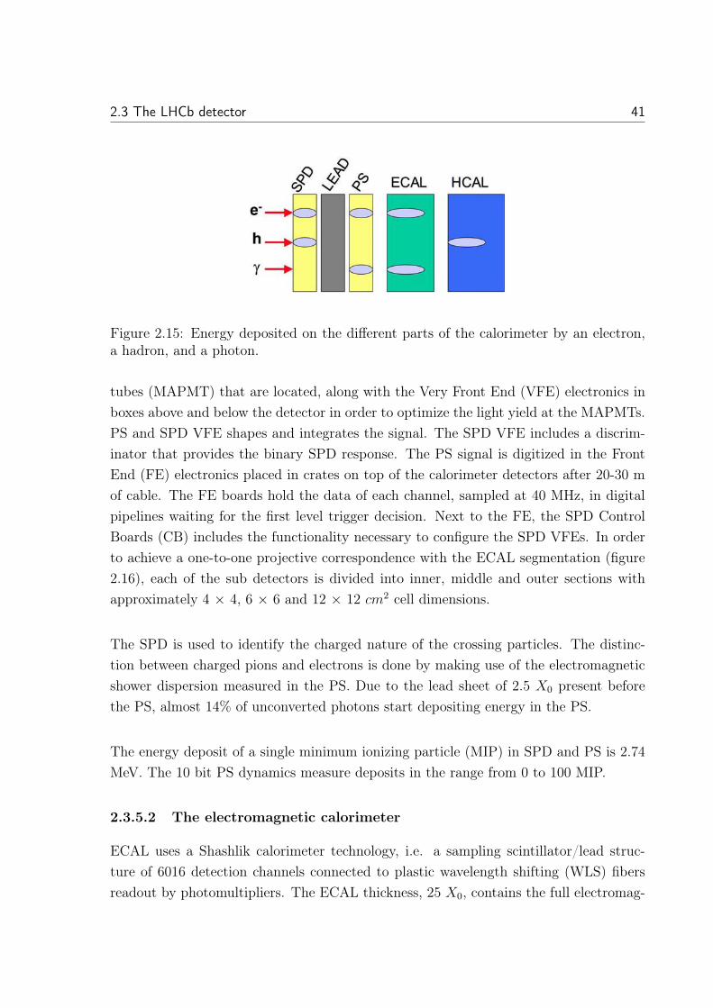
tromagnetic CALorimeter (ECAL) and the Hadronic CALorimeter (HCAL). The SPDand PS identify the charged and electromagnetic nature of the crossing particles, re-spectively. ECAL and HCAL measure the energy of the electromagnetic and hadronicshowering particles. The system is used at the first level trigger (L0) to rapidly separateelectrons, photons and hadrons. The interaction of the various types of particles in thecalorimeter is schematized in figure 2.15.
The calorimeter system play a major role in the reconstruction and selection of radiativedecays from trigger to offline analysis. At L0, photon candidates are reconstructed andselected with a transverse energy threshold of 2.5 GeV in 2011, 2.72 GeV in beginning2012 and 2.96 GeV in mid-2012.Almost 30 % of the photons coming from the interaction region convert in electron pairbefore reaching the calorimeter. Three categories of photons are reconstructed offline inLHCb depending whether they convert or not in the material upstream the calorimetersystem.
Unconverted photons and "late" conversions occurring after the magnet are recon-structed as a single energy deposit (cluster) in the ECAL as discussed in 3. Late con-version likely form a single ECAL cluster identified with SPD hits in front.The electron pair from photon conversion occurring before the magnet are reconstructed
40 The LHCb
��
��� � ���
�� ����
�����������
��������
Figure 2.14: Schema of the RICH detectors, RICH1 (left) and RICH2 (right).
by the tracking system.The invariant mass resolution of a B meson decaying to a final state with a photon -thephoton reconstructed as a calorimeter object- is completely dominated by the photonenergy resolution driven by the calorimeter. The invariant mass resolution of B → hhγ
is of the order of 90 MeV/c2 compared to that of B → hh which is of the order of 25MeV/c2. A good calibration of the calorimeter is an important prerequisite when doingradiative decays analysis.
The calorimeter system sub detectors are detailed in the following.
2.3.5.1 The Pad and the Preshower detectors
The SPD and PS are two planes of scintillator pads, with 6016 detection channels each,separated by a 15 mm, 2.5 X0, thick lead sheet. A groove in each pad holds the heli-coidal wavelength shifting (WLS) optical fiber which collects the scintillating light. Thetransmission of this light is done by long clear fibers to multi-anode photomultipliers
2.3 The LHCb detector 41
Figure 2.15: Energy deposited on the different parts of the calorimeter by an electron,a hadron, and a photon.
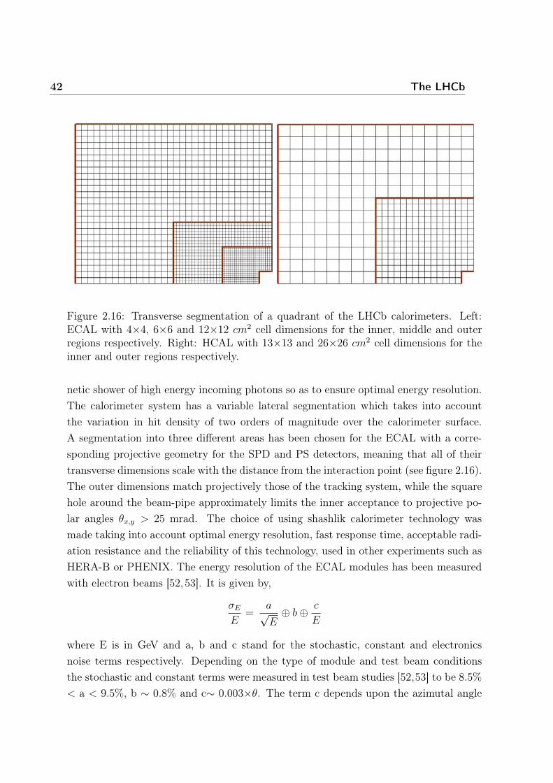
tubes (MAPMT) that are located, along with the Very Front End (VFE) electronics inboxes above and below the detector in order to optimize the light yield at the MAPMTs.PS and SPD VFE shapes and integrates the signal. The SPD VFE includes a discrim-inator that provides the binary SPD response. The PS signal is digitized in the FrontEnd (FE) electronics placed in crates on top of the calorimeter detectors after 20-30 mof cable. The FE boards hold the data of each channel, sampled at 40 MHz, in digitalpipelines waiting for the first level trigger decision. Next to the FE, the SPD ControlBoards (CB) includes the functionality necessary to configure the SPD VFEs. In orderto achieve a one-to-one projective correspondence with the ECAL segmentation (figure2.16), each of the sub detectors is divided into inner, middle and outer sections withapproximately 4 × 4, 6 × 6 and 12 × 12 cm2 cell dimensions.
The SPD is used to identify the charged nature of the crossing particles. The distinc-tion between charged pions and electrons is done by making use of the electromagneticshower dispersion measured in the PS. Due to the lead sheet of 2.5 X0 present beforethe PS, almost 14% of unconverted photons start depositing energy in the PS.
The energy deposit of a single minimum ionizing particle (MIP) in SPD and PS is 2.74MeV. The 10 bit PS dynamics measure deposits in the range from 0 to 100 MIP.
2.3.5.2 The electromagnetic calorimeter
ECAL uses a Shashlik calorimeter technology, i.e. a sampling scintillator/lead struc-ture of 6016 detection channels connected to plastic wavelength shifting (WLS) fibersreadout by photomultipliers. The ECAL thickness, 25 X0, contains the full electromag-
42 The LHCb
Figure 2.16: Transverse segmentation of a quadrant of the LHCb calorimeters. Left:ECAL with 4×4, 6×6 and 12×12 cm2 cell dimensions for the inner, middle and outerregions respectively. Right: HCAL with 13×13 and 26×26 cm2 cell dimensions for theinner and outer regions respectively.
netic shower of high energy incoming photons so as to ensure optimal energy resolution.The calorimeter system has a variable lateral segmentation which takes into accountthe variation in hit density of two orders of magnitude over the calorimeter surface.A segmentation into three different areas has been chosen for the ECAL with a corre-sponding projective geometry for the SPD and PS detectors, meaning that all of theirtransverse dimensions scale with the distance from the interaction point (see figure 2.16).The outer dimensions match projectively those of the tracking system, while the squarehole around the beam-pipe approximately limits the inner acceptance to projective po-lar angles θx,y > 25 mrad. The choice of using shashlik calorimeter technology wasmade taking into account optimal energy resolution, fast response time, acceptable radi-ation resistance and the reliability of this technology, used in other experiments such asHERA-B or PHENIX. The energy resolution of the ECAL modules has been measuredwith electron beams [52,53]. It is given by,
σE
E=
a√E
⊕ b⊕ c
E
where E is in GeV and a, b and c stand for the stochastic, constant and electronicsnoise terms respectively. Depending on the type of module and test beam conditionsthe stochastic and constant terms were measured in test beam studies [52,53] to be 8.5%< a < 9.5%, b ∼ 0.8% and c∼ 0.003×θ. The term c depends upon the azimutal angle
2.3 The LHCb detector 43
(θ) of the cell position with respect to the beam axis.
The ECAL is placed at 12.5m from the interaction point. Its dimensions match projec-tively those of the tracking system, θX < 300 mrad and θY < 250 mrad, but its inneracceptance is limited to θX,Y > 25 mrad due to the substantial radiation dose level inthat region.
The ECAL has a 12 bits dynamic range. The Analog-to-Digital Convertor (ADC) countsranging from 0 to 4095 and the point of zero energy being at 255 ADC counts. Themaximum energy per cell is limited by the possible gain applied to the PMTs and is7+10/sin(θ) GeV.
Calibration The performance of each of the cells of the ECAL can be slightly different,and they may suffer aging effects, i.e. detector material wearing out through out thepassage of time, at different rates. Therefore, it is necessary to regularly perform acalibration procedure to obtain a set of calibration coefficients, one per cell, in order toprovide the best possible operation from the whole calorimeter. In a first calibrationstage, the energy flow technique allows to even out the differences between neighboringcells by making use of the smoothness of the sum of transverse energy depositions inthe calorimeter. While this method allows to achieve a 5% calibration level, it cannotprovide a global energy scale for the calorimeter energy. Starting from the energy flowcalibration constants, the decay of resolved neutral pions into two photons is used toiteratively reach an inter calibration level of 2%. Since the calorimeter response is linear,the calibration with low energy π0 is valid to a good approximation at high energies. Thee/p ratio, where e is the calorimeter energy and p is the particle momentum measured bythe tracking system, is used to correct for aging effects over small periods correspondingto an integrated luminosity of 40 pb−1 in calorimeter areas [54,55].
2.3.5.3 The hadronic calorimeter
The HCAL is a sampling device made from iron and scintillating tiles, as absorber andactive material respectively. The scintillating tiles run parallel to the beam axis whichfacilitate the readout. The iron tiles are 16 mm thick while the scintillating ones are 4mm thick. The HCAL has a sampling fraction of 2.7% and corresponds to 5.6 interactionlengths which is not enough for containing the full hadronic shower. Therefore, it gives
44 The LHCb
only an estimation of the hadron energy with a design resolution of
σE
E=
70%√E
⊕ 10%
with E being in GeV. The HCAL saturates at E = 15/sinθ GeV. The HCAL is segmentedtransversely into square cells of 13 cm (inner) and 26 cm (outer), as illustrated in figure2.16.The energy resolution and uniformity of the HCAL were measured at the calorimetertest beam. From a lateral scan of a particle beam across the prototype front surface theuniformity in response was measured to be within ±3%. The resolution extracted froma fit to the data at several energies is also in agreement with the design values [56].
Calibration The calibration of the HCAL uses two 137Cs sources of almost 10mCi, oneper detector side. This procedure takes about an hour during which they are transportedthrough all of the scintillator cells by a hydraulic system. The response of the PMTs ismeasured by a dedicated system of current integrators. The relationship between theintegrated anode current and the particle energy was measured in test-beam and is usedto set the values for the HCAL parameters, obtaining a cell-to-cell inter-calibration atthe level of 5%. The use of the in-situ source limits the calibration procedure of theHCAL to technical stops, which occur bi-monthly.
The performance of the ECAL and the HCAL is monitored during the data-taking peri-ods using the built-in LED system. In addition, the distribution of e/p, for electrons inthe case of the ECAL, and h/p, for hadrons in the case of the HCAL, can be comparedto simulations and is used for monitoring purposes.
2.3.6 The Muon detector
Muon triggering and offline muon identification are fundamental requirements of theLHCb experiment. Muons are present in the final states of many CP-sensitive B decays,such as B0 → J/ψ(μ+μ−)K0
S or B0s → J/ψ(μ+μ−)φ, and also play a major role in CP
asymmetry and oscillation measurements in semileptonic decays, in which the muon canbe used to provide the tag of the initial flavor of the accompanying B meson. Further-more, muons are involved in rare B decays such as the flavor-changing neutral current
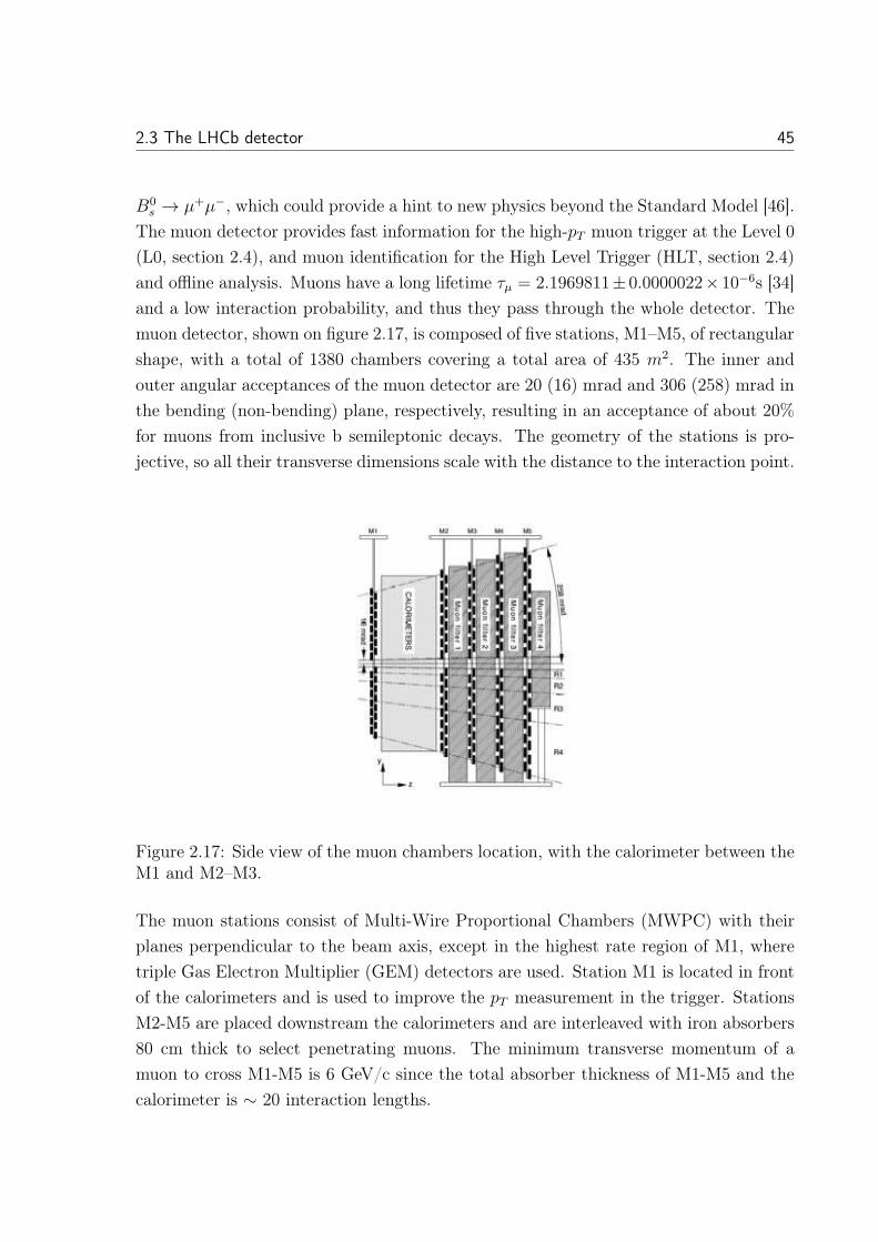
2.3 The LHCb detector 45
B0s → μ+μ−, which could provide a hint to new physics beyond the Standard Model [46].
The muon detector provides fast information for the high-pT muon trigger at the Level 0(L0, section 2.4), and muon identification for the High Level Trigger (HLT, section 2.4)and offline analysis. Muons have a long lifetime τμ = 2.1969811± 0.0000022× 10⁻⁶s [34]and a low interaction probability, and thus they pass through the whole detector. Themuon detector, shown on figure 2.17, is composed of five stations, M1–M5, of rectangularshape, with a total of 1380 chambers covering a total area of 435 m2. The inner andouter angular acceptances of the muon detector are 20 (16) mrad and 306 (258) mrad inthe bending (non-bending) plane, respectively, resulting in an acceptance of about 20%for muons from inclusive b semileptonic decays. The geometry of the stations is pro-jective, so all their transverse dimensions scale with the distance to the interaction point.
Figure 2.17: Side view of the muon chambers location, with the calorimeter between theM1 and M2–M3.
The muon stations consist of Multi-Wire Proportional Chambers (MWPC) with theirplanes perpendicular to the beam axis, except in the highest rate region of M1, wheretriple Gas Electron Multiplier (GEM) detectors are used. Station M1 is located in frontof the calorimeters and is used to improve the pT measurement in the trigger. StationsM2-M5 are placed downstream the calorimeters and are interleaved with iron absorbers80 cm thick to select penetrating muons. The minimum transverse momentum of amuon to cross M1-M5 is 6 GeV/c since the total absorber thickness of M1-M5 and thecalorimeter is ∼ 20 interaction lengths.
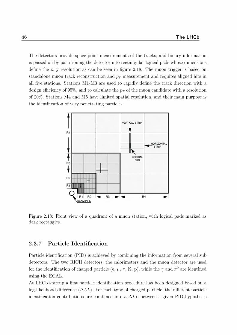
46 The LHCb
The detectors provide space point measurements of the tracks, and binary informationis passed on by partitioning the detector into rectangular logical pads whose dimensionsdefine the x, y resolution as can be seen in figure 2.18. The muon trigger is based onstandalone muon track reconstruction and pT measurement and requires aligned hits inall five stations. Stations M1-M3 are used to rapidly define the track direction with adesign efficiency of 95%, and to calculate the pT of the muon candidate with a resolutionof 20%. Stations M4 and M5 have limited spatial resolution, and their main purpose isthe identification of very penetrating particles.
Figure 2.18: Front view of a quadrant of a muon station, with logical pads marked asdark rectangles.
2.3.7 Particle Identification
Particle identification (PID) is achieved by combining the information from several subdetectors. The two RICH detectors, the calorimeters and the muon detector are usedfor the identification of charged particle (e, μ, π, K, p), while the γ and π0 are identifiedusing the ECAL.At LHCb startup a first particle identification procedure has been designed based on alog-likelihood difference (ΔLL). For each type of charged particle, the different particleidentification contributions are combined into a ΔLL between a given PID hypothesis
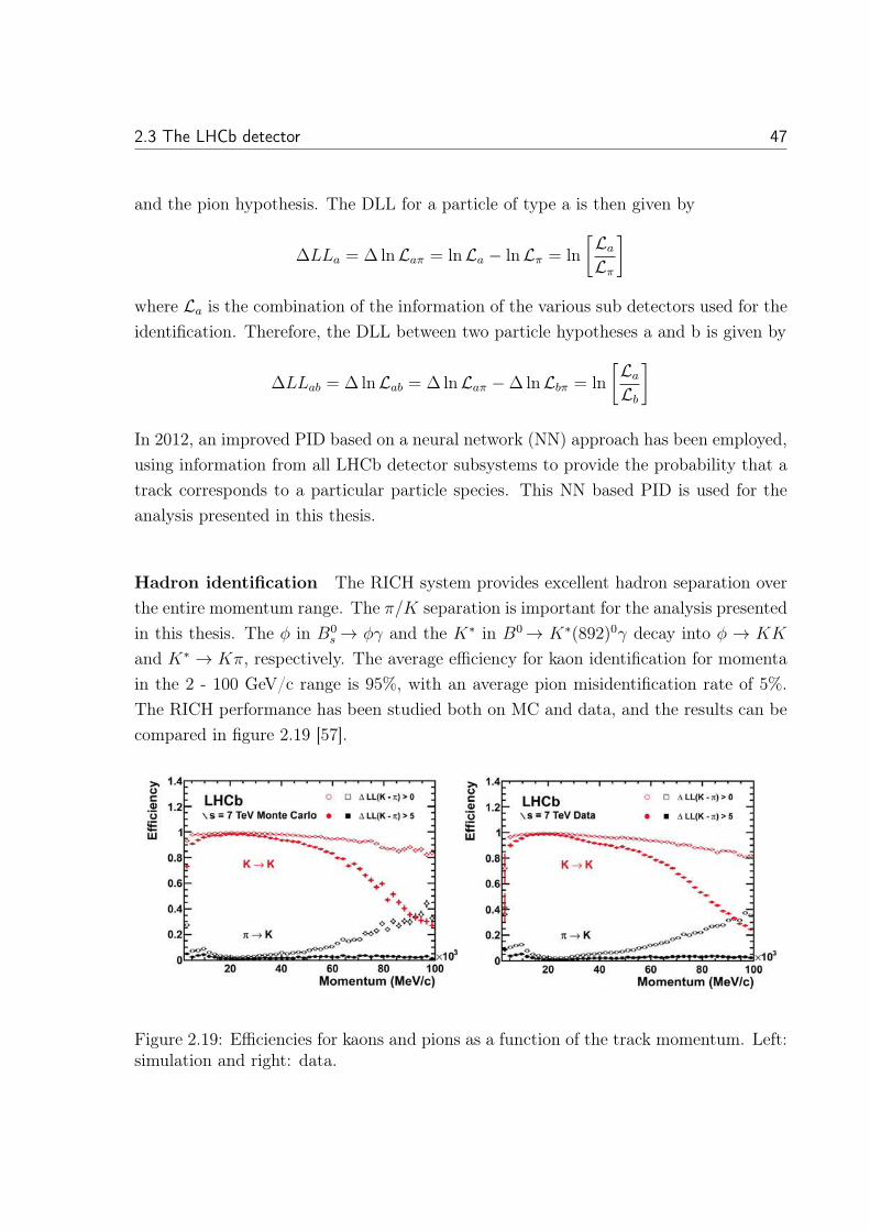
2.3 The LHCb detector 47
and the pion hypothesis. The DLL for a particle of type a is then given by
ΔLLa = Δ lnLaπ = lnLa − lnLπ = ln
[La
Lπ
]where La is the combination of the information of the various sub detectors used for theidentification. Therefore, the DLL between two particle hypotheses a and b is given by
ΔLLab = Δ lnLab = Δ lnLaπ −Δ lnLbπ = ln
[La
Lb
]
In 2012, an improved PID based on a neural network (NN) approach has been employed,using information from all LHCb detector subsystems to provide the probability that atrack corresponds to a particular particle species. This NN based PID is used for theanalysis presented in this thesis.
Hadron identification The RICH system provides excellent hadron separation overthe entire momentum range. The π/K separation is important for the analysis presentedin this thesis. The φ in B0
s → φγ and the K∗ in B0→ K∗(892)0γ decay into φ → KK
and K∗ → Kπ, respectively. The average efficiency for kaon identification for momentain the 2 - 100 GeV/c range is 95%, with an average pion misidentification rate of 5%.The RICH performance has been studied both on MC and data, and the results can becompared in figure 2.19 [57].
Figure 2.19: Efficiencies for kaons and pions as a function of the track momentum. Left:simulation and right: data.
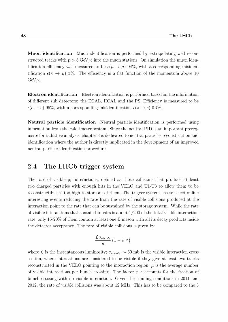
48 The LHCb
Muon identification Muon identification is performed by extrapolating well recon-structed tracks with p > 3 GeV/c into the muon stations. On simulation the muon iden-tification efficiency was measured to be ε(μ → μ) 94%, with a corresponding misiden-tification ε(π → μ) 3%. The efficiency is a flat function of the momentum above 10GeV/c.
Electron identification Electron identification is performed based on the informationof different sub detectors: the ECAL, HCAL and the PS. Efficiency is measured to beε(e → e) 95%, with a corresponding misidentification ε(π → e) 0.7%.
Neutral particle identification Neutral particle identification is performed usinginformation from the calorimeter system. Since the neutral PID is an important prereq-uisite for radiative analysis, chapter 3 is dedicated to neutral particles reconstruction andidentification where the author is directly implicated in the development of an improvedneutral particle identification procedure.
2.4 The LHCb trigger system
The rate of visible pp interactions, defined as those collisions that produce at leasttwo charged particles with enough hits in the VELO and T1-T3 to allow them to bereconstructible, is too high to store all of them. The trigger system has to select onlineinteresting events reducing the rate from the rate of visible collisions produced at theinteraction point to the rate that can be sustained by the storage system. While the rateof visible interactions that contain bb pairs is about 1/200 of the total visible interactionrate, only 15-20% of them contain at least one B meson with all its decay products insidethe detector acceptance. The rate of visible collisions is given by
Lσvisible
μ
(1− e−μ
)where L is the instantaneous luminosity; σvisible ∼ 60 mb is the visible interaction crosssection, where interactions are considered to be visible if they give at least two tracksreconstructed in the VELO pointing to the interaction region; μ is the average numberof visible interactions per bunch crossing. The factor e−μ accounts for the fraction ofbunch crossing with no visible interaction. Given the running conditions in 2011 and2012, the rate of visible collisions was about 12 MHz. This has to be compared to the 3
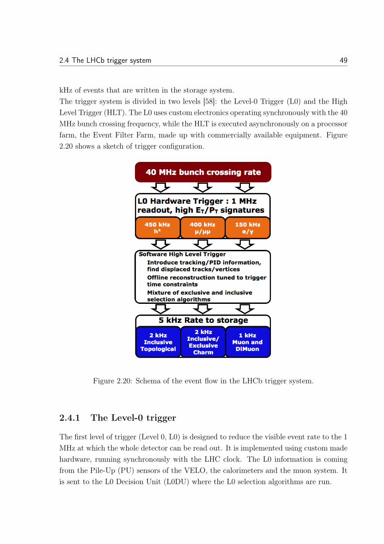
2.4 The LHCb trigger system 49
kHz of events that are written in the storage system.The trigger system is divided in two levels [58]: the Level-0 Trigger (L0) and the HighLevel Trigger (HLT). The L0 uses custom electronics operating synchronously with the 40MHz bunch crossing frequency, while the HLT is executed asynchronously on a processorfarm, the Event Filter Farm, made up with commercially available equipment. Figure2.20 shows a sketch of trigger configuration.
Figure 2.20: Schema of the event flow in the LHCb trigger system.
2.4.1 The Level-0 trigger
The first level of trigger (Level 0, L0) is designed to reduce the visible event rate to the 1MHz at which the whole detector can be read out. It is implemented using custom madehardware, running synchronously with the LHC clock. The L0 information is comingfrom the Pile-Up (PU) sensors of the VELO, the calorimeters and the muon system. Itis sent to the L0 Decision Unit (L0DU) where the L0 selection algorithms are run.
50 The LHCb
The PU system has been implemented to reject events with several primary vertices.It uses the information of the PU sensors of the VELO. Given that the experiment isrunning at higher μ than foreseen in the design, events with pile-up are not rejected. Itis used to trigger on beam-gas events providing the number of hits in the PU stations,which are the only detector elements upstream of the interaction point.The L0 calorimeter trigger system uses information from the four components of thecalorimeter, SPD, PS, ECAL and HCAL. It computes the transverse energy depositedin 2×2 calorimeter cells clusters. From these clusters, the following three types of can-didates are built. L0Hadron is the highest ET HCAL cluster added with the energy ofthe associated ECAL cluster. L0Photon is the highest ET ECAL cluster with an energythreshold of 5 MIP in the PS and no hit in the SPD cells corresponding to the PS cells.L0Electron has the same requirements as L0Photon, with the additional condition of atleast one SPD cell hit in front of the PS cells. The ET of each candidate is compared toa fixed threshold and events containing at least one candidate above threshold fire theL0 trigger. The total number of hits in the SPD is also determined, and is used to vetoevents that would take a disproportionately large fraction of the available processingtime in the HLT.The muon chambers perform a stand-alone muon reconstruction with a pT resolutionof ∼ 25%. Tracks are searched combining the pad data from the five muon stationsto form towers pointing towards the interaction region. The muon stations are dividedin quadrants and there is no exchange of information between the quadrants. In eachquadrant, the two muon candidates with highest pT are selected.
To select radiative decays, the event selection is triggered with L0Photon. Since around30% of the photons are converted into electrons before the SPD detector, the L0Electronchannel has to be incorporated as well to have a better efficiency.In L0, L0Electron and L0Photon select events with an electromagnetic deposit in theECAL with a transverse energy with respect to the beam direction, ET , greater than agiven threshold, placed at 2.5 GeV in 2011, 2.72 GeV beginning of 2012 and 2.96 GeVmid-2012. Additionally, a subset of the events that pass these two lines also pass theL0ElectronHi and L0PhotonHi lines, which require a higher ET value of 4.2 GeV.
2.4 The LHCb trigger system 51
2.4.2 The High Level Trigger
The High Level Trigger (HLT) filters events using a software application. It uses theOnline Event Filter Farm (EFF), which contains up to 20,000 CPU cores, to process andreduce the rate at which events are kept down to 3 kHz. The high rate of incoming eventsfrom the L0 trigger and the computing power limitation of the EFF do not allow theup-front use of the full event data information in the decision-making process. Thus, theHLT is divided in two stages: the first stage (HLT1) uses only a partial reconstructionto reduce the rate by a factor of 20 so that the second stage (HLT2) is able to performfull event reconstruction to further discriminate signal events. The HLT processing timeper event is close to 30 ms.
2.4.2.1 HLT1
The HLT1 is designed to minimize the impact of varying running conditions on its per-formance. It is based around a single track trigger, which searches for a single trackwith high momentum, a large impact parameter (IP, shortest distance between a trackand the primary vertex) with respect to all primary vertices (PV) in the event, and agood track quality [59]. the track should have an IP larger than 125 μm with respectto any PV, pT > 1.8 GeV/c and p > 12.5 GeV/c. For events triggered by the Level 0photon and electron lines, the pT requirement is relaxed to 0.8 GeV/c.HLT1 takes 15 ms to process an L0 accepted minimum bias event, and accepts 5% ofsuch events with an efficiency of more than 80% on signal events for most of LHCb’sbenchmark B decay modes [59,60]. The 50kHz selected by HLT1 are passed to HLT2.
In the HLT1, Hlt1TrackAllL0 and Hlt1TrackPhoton single track lines are the relevantlines for radiative B decays. They select events based on the transverse momentum ofthe tracks with respect to the beam direction and their impact parameter (IP, short-est distance between the track and the decay vertex). On one side, Hlt1TrackAllL0selects low-ET photons with a harder cut in the required track; on the other side,Hlt1TrackPhotonL0 allows to lower the transverse momentum requirement for the trackat the cost of a harder ET cut on the photon.
52 The LHCb
2.4.2.2 HLT2
The HLT2 input rate is sufficiently low to perform an almost-full-offline reconstruction,the main difference being that in the HLT2 only tracks with pT > 500 MeV/c and p> 5000 MeV/c are reconstructed. Having fully reconstructed events allows the HLT2trigger lines to use event selection criteria more in line with those used in offline analyses.Moreover, Global Event Cuts (GEC), such as the reconstructed track multiplicity, areused to reject complex events which require a big amount of processing time.The HLT2 runs exclusive and inclusive selections. The inclusive ones search for genericB decay features such as displaced vertices or dilepton pairs and the exclusive lines selectspecific decays using similar selections to those used offline. Special inclusive lines havebeen developed to trigger on partially reconstructed b-hadron decays. These so-calledtopological lines are based on displaced vertices with 2, 3 or 4 associated tracks. Thetopological lines were first implemented as cut based selections. Moreover, to improvethe performances, additional lines using a multivariate approach were then added [61,62].
In HLT2, two strategies, exclusive and inclusive, have been included to trigger on radia-tive B decays both with a relatively high efficiency.
The mean efficiency for the L0 muon triggers is evaluated to be about 90 %. The meanefficiency of the HLT to select decays with muons is about 80 %. The total triggerefficiency is then 70 % [63]. As for hadrons, the mean efficiency of the L0Hadron triggeris evaluated to be about 50 %, the HLT trigger efficiency to be 80 % and the totalefficiency to be about 40 % [63]. Whereas for the radiative decays trigger, the meanefficiency of the L0 trigger is about 60 %. At HLT, the efficiency is evaluated to bealmost 50 % resulting in a total trigger efficiency of 35 % [64].
2.5 The LHCb luminosity measurements
The number of selected events of a given process per unit of time, denoted asdn
dt, is
given by
dn
dt= σLε
where σ is the process cross section, L is the instantaneous luminosity and ε is the totalefficiency accounting for the detector acceptance as well as the reconstruction and selec-
2.6 The LHCb software 53
tion efficiencies.Hence, the determination of the luminosity is an essential cornerstone for the measure-ment of any cross section. The average instantaneous luminosity of two colliding bunchescan be expressed as
L =fN1N2
4πσxσy
where f is the revolution frequency (11245 Hz at the LHC), N1 and N2 are the numberof protons in the two bunches, σx and σy are the transverse sizes of the bunch at theinteraction point along the x and y axis respectively.AT LHCb two methods to determine the absolute luminosity have been implemented[65]: the Van der Meer scan in which the beams are moved in transverse directionsin order to investigate the beam transverse profiles counting the interaction rate as afunction of the beam offsets and the beam-imaging gas method where the high acceptanceof the VELO around the interaction point is used to reconstruct beam-gas verticesproduced by the collision of protons in the beam with molecules in the remaining gas ofthe beam pipe. The positions of the beam-gas interactions are used to determine beamangles and profiles [66]. Combining the two methods, the absolute luminosity can bedetermined with a relative precision of 3.5%, this allows to calculate a reference crosssection of visible interactions. Then, dedicated luminosity counters are defined in orderto follow the evolution of the instantaneous luminosity during the data taking. Figure2.3 shows the LHCb integrated luminosity accumulated over the 2011-2012 run period.
2.6 The LHCb software
The LHCb software is based on the Gaudi [67,68] architecture, which provides an ObjectOriented framework for all the applications used within the experiment [69]. It hasthe flexibility needed for running the LHCb chain from the Monte Carlo generation tothe real data analysis using the same tools. Data persistency is based on the Rootsoftware [70, 71], a set of object-oriented frameworks designed to handle and analyzelarge amounts of data.The simulation project is called GAUSS [72,73]. PYTHIA 6.4 [74] with a configurationspecific to LHCb is used to generate pp collisions. The hadronic particle decays aredescribed by the EvtGen [75] package in which PHOTOS [76] is used to generate finalstate radiations. GAUSS then connects the PYTHIA output as input of GEANT 4 [77]
54 The LHCb
which implements the interaction of the particles with the detector and the response ofthe active materials. The simulation of the digitization of the signals produced in theactive materials is performed by the BOOLE application [78]. It includes simulation ofthe readout electronics as well as of the L0 hardware trigger. The simulation output isdigitized data that mimics the real data coming from the detector.The event reconstruction is performed by the BRUNEL application [79]. The MOOREapplication [80] can be used to run the HLT selection on reconstructed events. This isespecially useful to emulate the HLT response on the simulated data. Finally, DAVINCI[81], the analysis application, computes for each event the variables used in the analysisand stores them in standard files.
2.7 Data flow in LHCb
The raw data of the events selected by the trigger system coming from the experiment aretransferred to the CERN Tier-0 for further processing and archiving. These unprocesseddata are then used to reconstruct the physical particles, made up from tracks and particleidentification information, by making use of the raw information such as the hits or thecalorimeter cluster energies. This reconstruction process is performed in the Tier-1’s.Reconstructed events are saved in a Stripping Data Summary Tape (SDST) file, whichcontains the necessary information for further event filtering without including the rawdata.The SDST files are analyzed in order to further filter events for physical analyses bymaking use of the full reconstructed information and with looser timing constraints thanin the HLT. This sequence is known as Stripping, and finally produces a Data SummaryTape (DST) file, to which the raw data event information is attached. DSTs are the filesaccessible to scientists for physics analyses. The data are reprocessed several times ayear with the improvement of the reconstruction, alignment and stripping software andalgorithms.
Chapter 3
Photon reconstruction andidentification
Contents3.1 Photon reconstruction . . . . . . . . . . . . . . . . . . . . . . 56
3.1.1 Clusterization . . . . . . . . . . . . . . . . . . . . . . . . . . . . 56
3.1.2 Neutral clusters selection . . . . . . . . . . . . . . . . . . . . . 57
3.1.3 Photon reconstruction . . . . . . . . . . . . . . . . . . . . . . . 57
3.2 π0 reconstruction . . . . . . . . . . . . . . . . . . . . . . . . . . 59
3.2.1 Resolved π0 . . . . . . . . . . . . . . . . . . . . . . . . . . . . . 59
3.2.2 Merged π0 . . . . . . . . . . . . . . . . . . . . . . . . . . . . . . 60
3.3 Multivariate approaches . . . . . . . . . . . . . . . . . . . . . 60
3.4 Photon identification . . . . . . . . . . . . . . . . . . . . . . . 63
3.4.1 The ΔLL based Photon identification . . . . . . . . . . . . . . 63
3.4.2 Improved Photon identification . . . . . . . . . . . . . . . . . . 65
3.5 γ/π0 separation . . . . . . . . . . . . . . . . . . . . . . . . . . . 76
3.5.1 Calibration with real data . . . . . . . . . . . . . . . . . . . . . 83
55
56 Photon reconstruction and identification
The detection of photons and neutral pions decaying into photons pair is per-formed by the LHCb Electromagnetic CALorimeter (ECAL). Moreover, and in orderto have a precise determination of photon parameters, information from the PreShower(PS) and the Silicon Pad Detector (SPD) detectors are used. In this chapter, the re-construction technique of photons will be described in details, then, the procedure forphoton identification will be discussed. Also, photon and neutral pion separation will beexplained and discussed.
3.1 Photon reconstruction
3.1.1 Clusterization
The reconstruction of electromagnetic showers process begins with the identification ofthe ECAL cell that has an excess in energy deposition, referred to as local maximumor seed cell, compared to all its direct neighbors. The number of neighbor cells is 8 per’regular’ cells which are far from boundaries of ECAL areas, and it varies from 3 to 9for cells near the boundaries. These cells are selected only if the transverse energy islarger than 50 MeV [82]. The identified cell will originate the cluster according to theclusterisation procedure adopted by the Cellular Automaton algorithm [83]. As directconsequence of these formal definitions, the seed cells of two reconstructed clusters arealways separated at least by one cell. If a calorimeter cell is shared between two clustersthe energy of the cell is shared between the clusters depending on the total cluster energyand the distance between the clusters’ barycenter.The transversal barycenter and energy of the electromagnetic shower deposit in theECAL of the corresponding particle are calculated as
ε =∑i
εi xb =1
ε
∑i
xiεi yb =1
ε
∑i
yiεi
where εi represents the energy measured in each cell i of the cluster, xi and yi give theposition of the center of the cell. A 3 × 3 mask is applied around the seed cell for theevaluation ε and the transversal barycenter to limit the accumulation of electronic noise.
3.1 Photon reconstruction 57
3.1.2 Neutral clusters selection
The selection of neutral clusters are performed using an anti-matching techniques withreconstructed tracks. Reconstructed tracks in the event are extrapolated to the calorime-ter and then all-to-all matching with the reconstructed clusters are performed. A two-dimensional χ2
2D is then constructed as
χ22D(�P ) =
(�Ptr − �P
)TC−1tr
(�Ptr − �P
)+(�Pcl − �P
)TS−1
(�Pcl − �P
)where �Ptr is the extrapolated track 2D-point to the calorimeter plane, Ctr is the co-variance matrix of �Ptr parameters, �Pcl is cluster barycenter position and S is the corre-sponding 2×2 covariance matrix. The χ2
2D is minimized with respect to �P . The clusterswith minimal value of χ2
2D estimator in excess of 4 are selected as neutral clusters. Thiscriteria rejects the clusters due to electrons and significantly suppress the clusters dueto other charged particles keeping the high efficiency for clusters due to photons.
3.1.3 Photon reconstruction
There are two types of photons considered at LHCb, converted and unconverted. Due tothe material found between the interaction point and the calorimeter, 30% of the photonscoming from the interaction region convert into a e+e− pair before the calorimeter frontface. There are two kinds of converted photons. If the photon conversion occurs beforethe tracking system, the tracks of the two electrons can be reconstructed. Then thephoton information is coming from the reconstruction of the two separated electronstracks. If the conversion happens after the magnet, the electrons mostly end up in asingle ECAL cluster and the charged nature of the conversion can be identified usingthe signal left in the SPD. A cluster with no matching tracks but with a deposit in theSPD is the signature of a converted photon after the magnet. Dedicated correctionsexplained later are determined for converted photons.
3.1.3.1 Photon energy
The geometry of the calorimeter system has been chosen in such a way that the ECALcells correspond to the PS and SPD cells. The photon energy is evaluated by summingthe ECAL cluster energy with the energy deposit in the PS cells in front. The mainenergy loss comes from the fact that the cluster is reconstructed as a 3×3 matrix of ECAL
58 Photon reconstruction and identification
cells and the transversal energy deposited outside this matrix of cells is not accountedfor. Moreover, the dead material between the modules of the calorimeter cells introducesintrinsic losses that need to be compensated. These leakages are corrected following
E(γ) = αEECAL + βEPS
where EPS is the measured energy in the PS cells. The factor α is obtained from thephotons subsample with small energy deposits in the PS and it accounts for lateraland longitudinal leakages in the ECAL and the relative position of the energy-weightedbarycenter inside the cluster and inside the ECAL module frame. The passive-to-activeenergy -being the energy measured in the scintillator to that radiated in the lead- factorβ for PS is obtained from the complementary subsample once α is determined.
3.1.3.2 Photon momentum
The transversal barycenter of the shower, xc, yc, is evaluated from the energy-weightedbarycenter of the cluster (section 3.1.1) corrected from the non linear transversal profileof the shower shape (hereafter referred to as S-correction). Assuming the transversalshower shape fit with a single exponential, E(r) ∼ E0e
−r/b, the S-corrected barycenter,xc, yc, is then given by the single parameter S-function [84]
(xc, yc) = S0 [(xb , yb), b] = b asinh
[(xb , yb)
Δcosh
Δ
b
]where (xb , yb) are the x,y positions of the energy-weighted barycenter, Δ the half cellsize and b the decay constant of the exponential profile. The b parameter is tuned ondata using electron tracks matched clusters. It is found to be about 10%, 13% and 15%of the cell size for the outer, middle and inner ECAL regions, respectively.Moreover, the transversal barycenter position has to be corrected from left/right asym-metries in the X-direction (bottom/up in the Y-direction) that is due to the incidenceangle of the photon that induces a non spherical profile of the shower spot, also, andsince the single exponential is a rough approximation, an additional corrections to S0 isneeded; the S-correction is
(xc, yc) = S0 [(xb , yb), b] + S1 [(xb , yb)] + S2 [(xb , yb)]
having S1 and S2 as correcting from residual S-shape and geometrical asymmetries, re-
3.2 π0 reconstruction 59
spectively and improving the resolution on the impact position of the photon [85].
The first evaluation of the photon momentum is done assuming its origin is (0,0,0).When this photon is associated to a decay, its parameters are reevaluated according tothe decay vertex. The photon direction is pointing to the 3D barycenter of the showerxc, yc and zc. zc is obtained as the ECAL position corrected from the penetration depthof the photon. The correction is scaled as the logarithm of the energy and, in order totake into account the information provided by the PS about the position of the showerbeginning, a smooth dependance of the parameter βc with EPS is included
zc = zECAL + αc ln(Ec) + βc(EPS )
3.2 π0 reconstruction
π0 branching fraction into two photons is (98.823±0.034)% [86]. The π0 signature in theECAL depends on its kinematics, the higher is the momentum of the π0 the closer thetwo photons are at the entry of the calorimeter. These two photons can then producetwo separated clusters or share a single cluster in which their individual signals are notclearly distinguishable. The π0 are classified as resolved π0 in the former case and asmerged π0 in the latter one. The transverse momentum spectrum of merged π0 startsaround 2 GeV/c.
3.2.1 Resolved π0
To reconstruct resolved π0, photons are paired and their invariant mass, mγγ, is comparedwith the π0 mass. Only photons with transverse momentum greater than 200 MeV/c andwith a track matching χ2
2D greater than 4 are taken into account [85]. mγγ is required tobe in the range 105 to 165 MeV/c2. The measured resolution of mγγ is about 7 MeV/c2
in the 2011-2012 sample. Using those criteria and according to the simulation, the globalreconstruction and identification efficiency of resolved π0, with respect to events whereboth photons are in the ECAL acceptance, both with transverse momentum greaterthan 200 MeV/c, is about 50% [85]. The inefficiency is mostly due to photon showeringin the material upstream the calorimeter. Part of this inefficiency can be measured byconsidering photon conversion reconstructed as a pair of electrons.
60 Photon reconstruction and identification
3.2.2 Merged π0
Each electromagnetic cluster is split in two subclusters defined from the two most en-ergetic cells in the cluster. An algorithm calculates the barycenter of each sub clusterusing the expected transverse shower shape of individual photons. The positions of thetwo barycenters depend on the energy sharing between the two subclusters, which itselfdepends on the positions of the two barycenters. According to that, the calculation isdone using an iterative procedure [85].
After the preparation of the two photon subclusters, the following criteria are appliedto identify the cluster as coming from a π0.
• The cluster is identified as coming from a neutral particle requiring a track match-ing χ2
2D > 1.
• The cluster energy has to be compatible with the merged π0 hypothesis. To assurethat, a cut is applied on the minimal distance allowed by the kinematics betweenthe impacts of the two photons on the ECAL front face
dγγ = 2× zECAL ×mπ0/Eπ0 < 1.8Δ,
where Δ is the transverse size of the calorimeter cell, mπ0 is fixed to 135 MeV ,Eπ0 is the π0 energy and zECAL is the position of the ECAL front face with respectto the interaction point.
• The reconstructed merged π0 mass is required to be in the range 75 to 195 MeV/c2.The wider mass range compared to resolved π0 is due to the higher mγγ resolutionof 12-15 MeV/C2.
The performance of neutral pion reconstruction is illustrated in figure 3.1, which showsthe invariant mass distribution for D0 → K−π+π0 candidates for resolved and mergedπ0 candidates [87]. In this example, the estimated resolution of the invariant mass ofthe reconstructed D0 is 30 MeV/c for the merged π0 candidates and 20 MeV/c for theresolved ones.
3.3 Multivariate approaches
Particle identification algorithms at LHCb are based on multivariate approaches. Mul-tivariate classifiers combine correlated input variables into a discriminant output. They
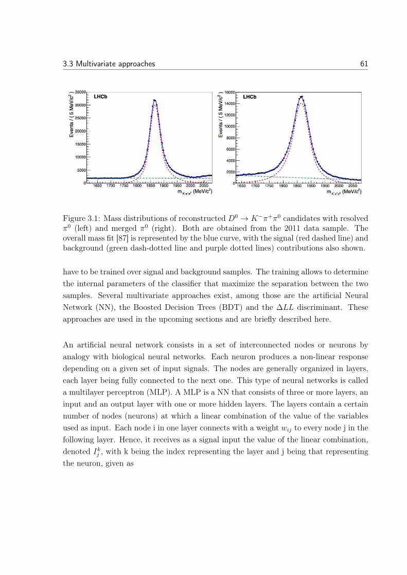
3.3 Multivariate approaches 61
Figure 3.1: Mass distributions of reconstructed D0 → K−π+π0 candidates with resolvedπ0 (left) and merged π0 (right). Both are obtained from the 2011 data sample. Theoverall mass fit [87] is represented by the blue curve, with the signal (red dashed line) andbackground (green dash-dotted line and purple dotted lines) contributions also shown.
have to be trained over signal and background samples. The training allows to determinethe internal parameters of the classifier that maximize the separation between the twosamples. Several multivariate approaches exist, among those are the artificial NeuralNetwork (NN), the Boosted Decision Trees (BDT) and the ΔLL discriminant. Theseapproaches are used in the upcoming sections and are briefly described here.
An artificial neural network consists in a set of interconnected nodes or neurons byanalogy with biological neural networks. Each neuron produces a non-linear responsedepending on a given set of input signals. The nodes are generally organized in layers,each layer being fully connected to the next one. This type of neural networks is calleda multilayer perceptron (MLP). A MLP is a NN that consists of three or more layers, aninput and an output layer with one or more hidden layers. The layers contain a certainnumber of nodes (neurons) at which a linear combination of the value of the variablesused as input. Each node i in one layer connects with a weight wij to every node j in thefollowing layer. Hence, it receives as a signal input the value of the linear combination,denoted Ikj , with k being the index representing the layer and j being that representingthe neuron, given as
62 Photon reconstruction and identification
Ikj =∑i
wijOk−1i
with,
Okj = g(Ikj )
being the value assigned to each neuron j in the layer k with O1j = λj where λ is the
value of the input variable. g is the activation function of a node which defines its outputgiven an input or set of inputs. The used activation function is of the type sigmoid. Therole of the weights that are applied to the neural net between the input layer and thefirst hidden layer is to construct linear combinations of the input variables in such a wayas to separate two types of classes, giving one of them high positive values of the linearcombination and giving the other low negative values. Hence, the global informationthat is present at the input layer is propagated via the hidden layers to the output layer(forward propagation). The value of the output neuron presents the best separationbetween the two classes of object’s.
The learning phase (training phase) of the NN consists in adjusting the weights in orderto achieve the optimal separation. When the number of training cycles is large that, inthe limit of a finite training sample, the pattern recognition is fine tuned for events inthe training sample and give worse performance on a different sample, the classifier issaid to be overtrained. Learning is based on an algorithm that necessitate the activationfunction to be continuous and differentiable. When the neural net is used to separatetwo overlapping classes of objects in the variable space, the continuity of the transferfunction permits to consider the neural net as an approximation of an ideal classifierbased on the probability that the events belongs to certain class. In the NN, the prob-ability density of a certain class is deduced throughout the learning phase and need notbe known in advance [88].Hence, each object is presented to the NN and the weights are adjusted accordingly. Theprocedure is repeated iteratively for many times where each iteration defines a learningcycle.The weight correction applied to the weights associated to the layers n-1 and n take intoaccount the corrections applied to the weights associated to the layers n and n+1, hencebackpropagating the error from the output layer through the hidden layers to the inputlayer.
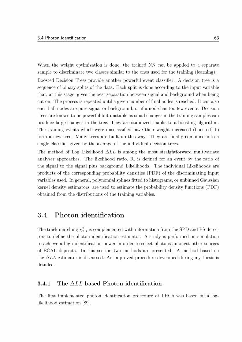
3.4 Photon identification 63
When the weight optimization is done, the trained NN can be applied to a separatesample to discriminate two classes similar to the ones used for the training (learning).
Boosted Decision Trees provide another powerful event classifier. A decision tree is asequence of binary splits of the data. Each split is done according to the input variablethat, at this stage, gives the best separation between signal and background when beingcut on. The process is repeated until a given number of final nodes is reached. It can alsoend if all nodes are pure signal or background, or if a node has too few events. Decisiontrees are known to be powerful but unstable as small changes in the training samples canproduce large changes in the tree. They are stabilized thanks to a boosting algorithm.The training events which were misclassified have their weight increased (boosted) toform a new tree. Many trees are built up this way. They are finally combined into asingle classifier given by the average of the individual decision trees.
The method of Log Likelihood ΔLL is among the most straightforward multivariateanalyser approaches. The likelihood ratio, R, is defined for an event by the ratio ofthe signal to the signal plus background Likelihoods. The individual Likelihoods areproducts of the corresponding probability densities (PDF) of the discriminating inputvariables used. In general, polynomial splines fitted to histograms, or unbinned Gaussiankernel density estimators, are used to estimate the probability density functions (PDF)obtained from the distributions of the training variables.
3.4 Photon identification
The track matching χ22D is complemented with information from the SPD and PS detec-
tors to define the photon identification estimator. A study is performed on simulationto achieve a high identification power in order to select photons amongst other sourcesof ECAL deposits. In this section two methods are presented. A method based onthe ΔLL estimator is discussed. An improved procedure developed during my thesis isdetailed.
3.4.1 The ΔLL based Photon identification
The first implemented photon identification procedure at LHCb was based on a log-likelihood estimation [89].

64 Photon reconstruction and identification
3.4.1.1 Samples definition
Performance evaluation and separation optimization is performed on simulated data(MC). For that purpose, signal and background samples are defined in the followingway:
Signal: a reconstructed photon that is associated to a simulated (MC) photon origi-nating from the interaction region defined by (Δr ≤ 10mm,Δz ≤ 150mm) and whoseenergy is correctly measured in the interval
ΔE =‖Eγ
Rec − EγMC‖
EγRec
≤ 25%.
Background: all reconstructed photon candidates that do not match signal definition.
It is worth noting that the background sample contains real photons not originatingfrom the interaction region.
3.4.1.2 Discriminating variables
The main variable used for this photon identification tool is the χ22D of the cluster. In
addition, the energy deposits in the PS of the calorimeter system is also used. The PSenergy deposit is high for particles interacting electromagnetically and allows an efficientseparation of the signal with charged pion background [89].The χ2
2D of the cluster (section 3.1.1) permits to apply an accurate track veto and toremove a large fraction of the electron background which is not identified by the SPDcriteria. The background is very high for small χ2
2D value, although the signal is notparticularly peaked.The photons distributions are built separately for converted, i.e. having an SPD sig-nal in the cell facing the calorimeter cluster center, or not and histograms where builtfor each photon energy interval. The Probability Density Functions (PDF) where builtfor each photon energy bin. This was necessary to improve the selection efficiency asthe distributions of the variables of interest depend on the cluster reconstructed energy.The energy bin width depends on the statistics in the energy region considered in orderto populate the distributions and on the rapidity of the variations of the variables withrespect to the energy. The non-constant bin size is to have a similar statistics in each bin.
The variables are combined as follows
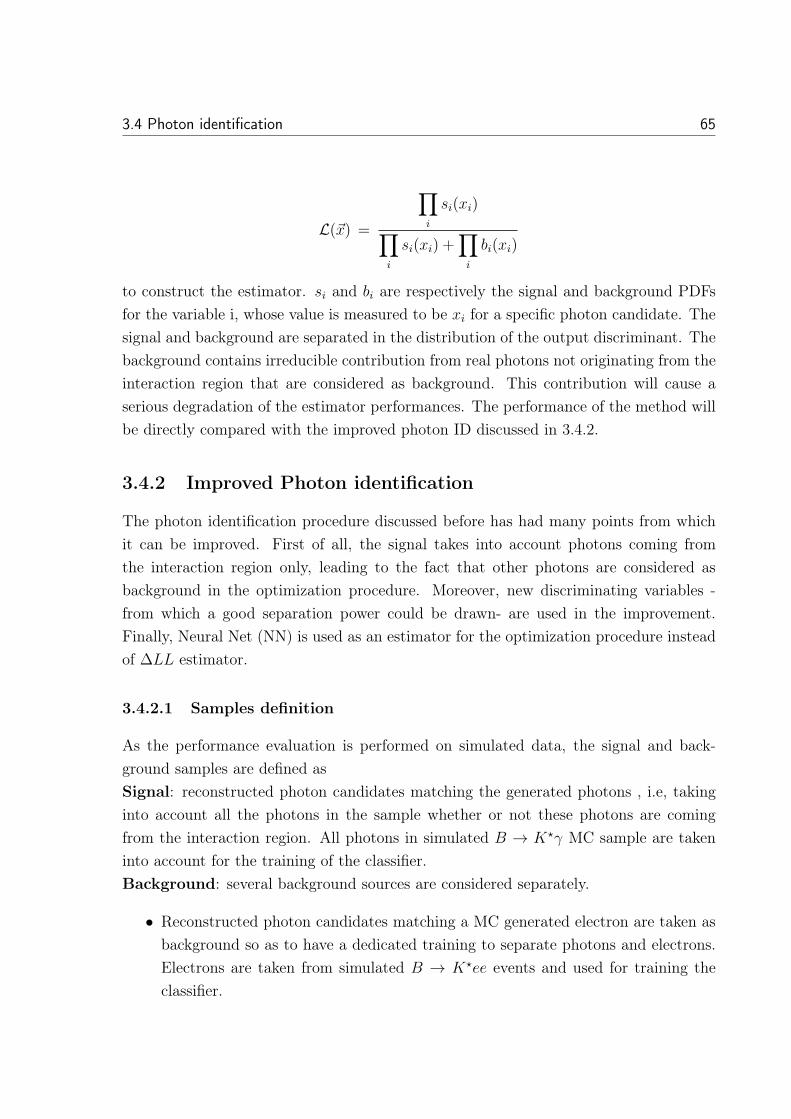
3.4 Photon identification 65
L(�x) =
∏i
si(xi)∏i
si(xi) +∏i
bi(xi)
to construct the estimator. si and bi are respectively the signal and background PDFsfor the variable i, whose value is measured to be xi for a specific photon candidate. Thesignal and background are separated in the distribution of the output discriminant. Thebackground contains irreducible contribution from real photons not originating from theinteraction region that are considered as background. This contribution will cause aserious degradation of the estimator performances. The performance of the method willbe directly compared with the improved photon ID discussed in 3.4.2.
3.4.2 Improved Photon identification
The photon identification procedure discussed before has had many points from whichit can be improved. First of all, the signal takes into account photons coming fromthe interaction region only, leading to the fact that other photons are considered asbackground in the optimization procedure. Moreover, new discriminating variables -from which a good separation power could be drawn- are used in the improvement.Finally, Neural Net (NN) is used as an estimator for the optimization procedure insteadof ΔLL estimator.
3.4.2.1 Samples definition
As the performance evaluation is performed on simulated data, the signal and back-ground samples are defined asSignal: reconstructed photon candidates matching the generated photons , i.e, takinginto account all the photons in the sample whether or not these photons are comingfrom the interaction region. All photons in simulated B → K γ MC sample are takeninto account for the training of the classifier.Background: several background sources are considered separately.
• Reconstructed photon candidates matching a MC generated electron are taken asbackground so as to have a dedicated training to separate photons and electrons.Electrons are taken from simulated B → K ee events and used for training theclassifier.
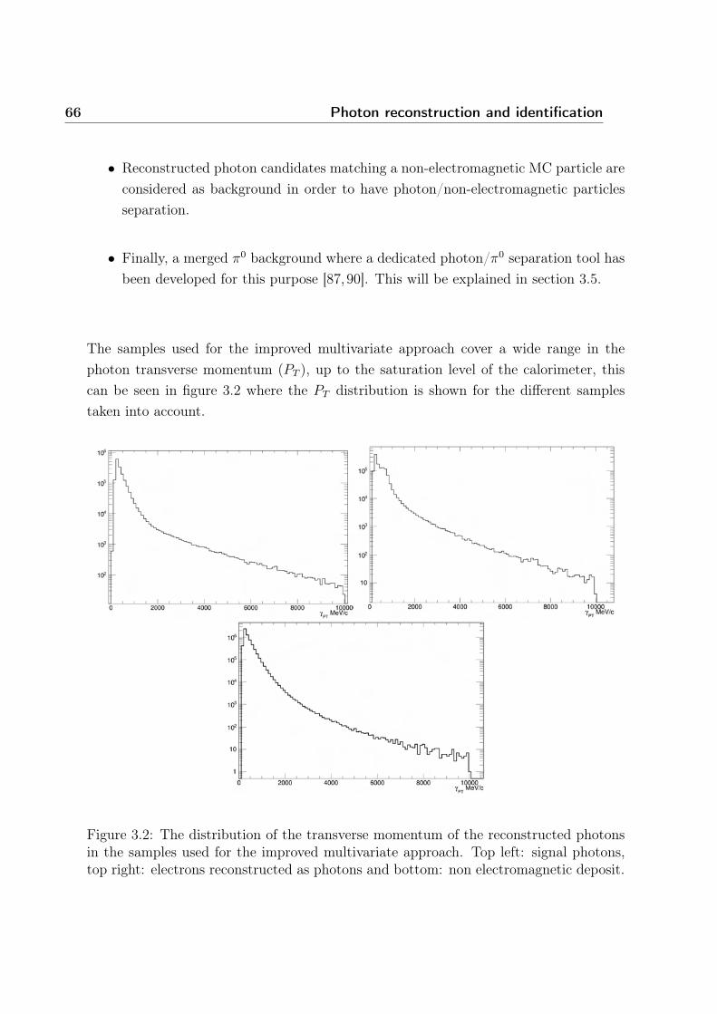
66 Photon reconstruction and identification
• Reconstructed photon candidates matching a non-electromagnetic MC particle areconsidered as background in order to have photon/non-electromagnetic particlesseparation.
• Finally, a merged π0 background where a dedicated photon/π0 separation tool hasbeen developed for this purpose [87,90]. This will be explained in section 3.5.
The samples used for the improved multivariate approach cover a wide range in thephoton transverse momentum (PT ), up to the saturation level of the calorimeter, thiscan be seen in figure 3.2 where the PT distribution is shown for the different samplestaken into account.
Figure 3.2: The distribution of the transverse momentum of the reconstructed photonsin the samples used for the improved multivariate approach. Top left: signal photons,top right: electrons reconstructed as photons and bottom: non electromagnetic deposit.

3.4 Photon identification 67
3.4.2.2 Discriminating variables
The improved multivariate separation uses the same set of variables described in section3.4.1.2 together with new discriminating variables described below
• The ratio of the energy of the seed cell to that of the total cluster in the ECAL:(Eseed/E3×3)ECAL.
• The ratio of the energy in the PS cell in front of the seed cell to that of the totalPS energy: (E1/E3×3)PS.
• The ratio of the energy in the HCAL, in the projective area matching the cluster,to the energy in the ECAL: EHCAL/EECAL.
• The 2× 2 matrix of PS cells with the highest energy deposit in front of the 3× 3
reconstructed cluster: PSE4Max.
• The second order energy-weighted momentum of the cluster defined from
SXX =
∑Ni=1 ei(xi − xc)
2∑Ni=1 ei
,
SY Y =
∑Ni=1 ei(yi − yc)
2∑Ni=1 ei
,
SXY = SY X =
∑Ni=1 ei(xi − xc)(yi − yc)∑N
i=1 ei
where (xc, yc) is the position of the photon defined in section 3.1. The clusterspread is defined as SXX + SY Y
• The number of PS cells in front of the cluster with non-zero energy deposit: PS-Multi.
• The multiplicity of hits in the 3× 3 SPD cells matrix in front of the reconstructedcluster: SPDMulti.
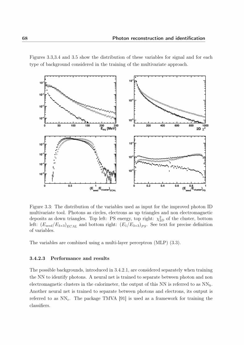
68 Photon reconstruction and identification
Figures 3.3,3.4 and 3.5 show the distribution of these variables for signal and for eachtype of background considered in the training of the multivariate approach.
Figure 3.3: The distribution of the variables used as input for the improved photon IDmultivariate tool. Photons as circles, electrons as up triangles and non electromagneticdeposits as down triangles. Top left: PS energy, top right: χ2
2D of the cluster, bottomleft: (Eseed/E3×3)ECAL and bottom right: (E1/E3×3)PS. See text for precise definitionof variables.
The variables are combined using a multi-layer perceptron (MLP) (3.3).
3.4.2.3 Performance and results
The possible backgrounds, introduced in 3.4.2.1, are considered separately when trainingthe NN to identify photons. A neural net is trained to separate between photon and nonelectromagnetic clusters in the calorimeter, the output of this NN is referred to as NNh.Another neural net is trained to separate between photons and electrons, its output isreferred to as NNe. The package TMVA [91] is used as a framework for training theclassifiers.
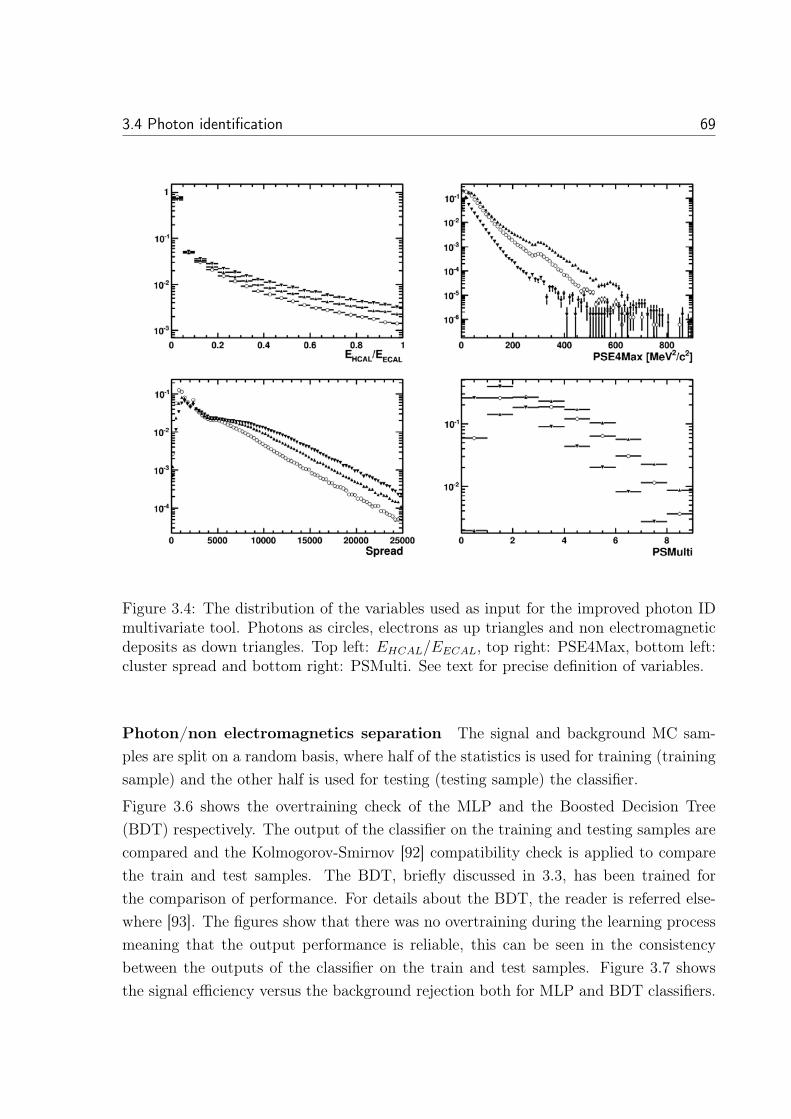
3.4 Photon identification 69
Figure 3.4: The distribution of the variables used as input for the improved photon IDmultivariate tool. Photons as circles, electrons as up triangles and non electromagneticdeposits as down triangles. Top left: EHCAL/EECAL, top right: PSE4Max, bottom left:cluster spread and bottom right: PSMulti. See text for precise definition of variables.
Photon/non electromagnetics separation The signal and background MC sam-ples are split on a random basis, where half of the statistics is used for training (trainingsample) and the other half is used for testing (testing sample) the classifier.
Figure 3.6 shows the overtraining check of the MLP and the Boosted Decision Tree(BDT) respectively. The output of the classifier on the training and testing samples arecompared and the Kolmogorov-Smirnov [92] compatibility check is applied to comparethe train and test samples. The BDT, briefly discussed in 3.3, has been trained forthe comparison of performance. For details about the BDT, the reader is referred else-where [93]. The figures show that there was no overtraining during the learning processmeaning that the output performance is reliable, this can be seen in the consistencybetween the outputs of the classifier on the train and test samples. Figure 3.7 showsthe signal efficiency versus the background rejection both for MLP and BDT classifiers.
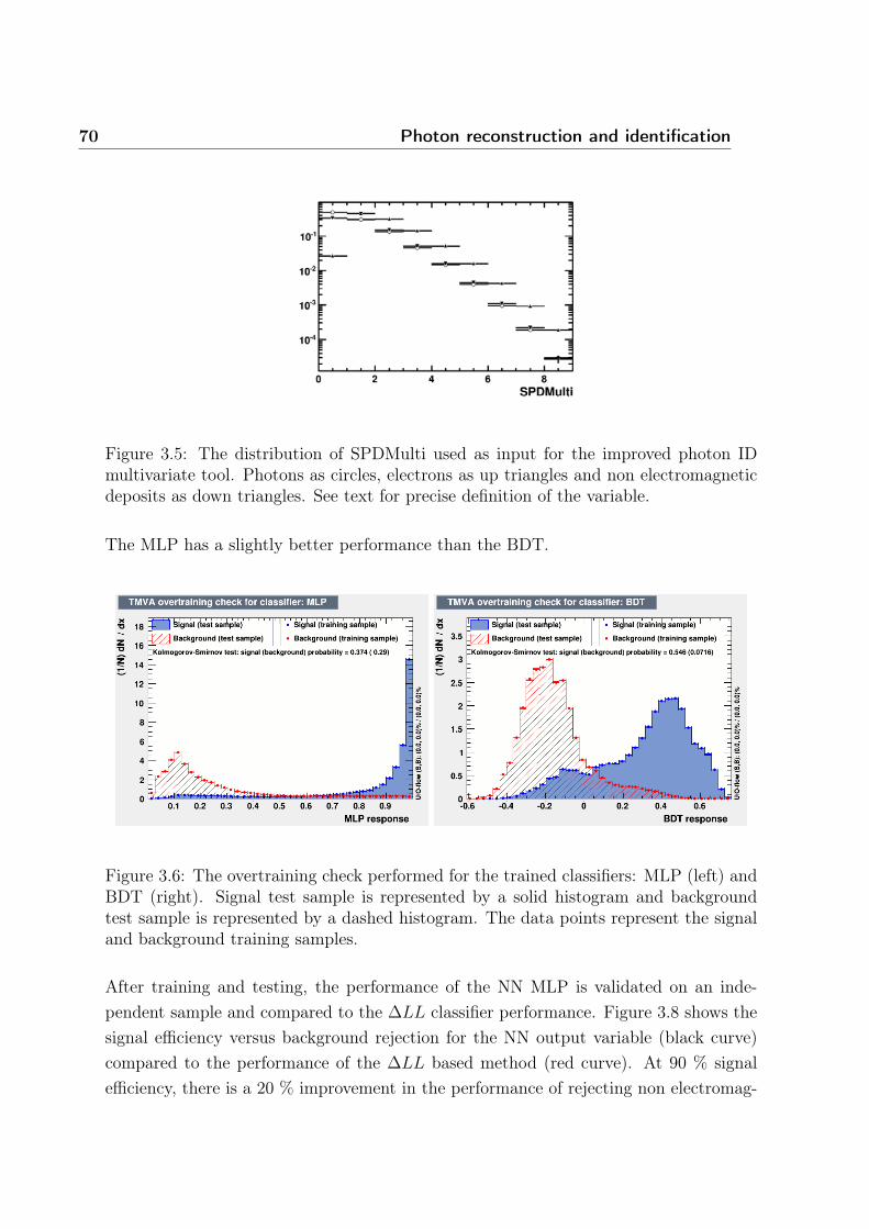
70 Photon reconstruction and identification
Figure 3.5: The distribution of SPDMulti used as input for the improved photon IDmultivariate tool. Photons as circles, electrons as up triangles and non electromagneticdeposits as down triangles. See text for precise definition of the variable.
The MLP has a slightly better performance than the BDT.
Figure 3.6: The overtraining check performed for the trained classifiers: MLP (left) andBDT (right). Signal test sample is represented by a solid histogram and backgroundtest sample is represented by a dashed histogram. The data points represent the signaland background training samples.
After training and testing, the performance of the NN MLP is validated on an inde-pendent sample and compared to the ΔLL classifier performance. Figure 3.8 shows thesignal efficiency versus background rejection for the NN output variable (black curve)compared to the performance of the ΔLL based method (red curve). At 90 % signalefficiency, there is a 20 % improvement in the performance of rejecting non electromag-
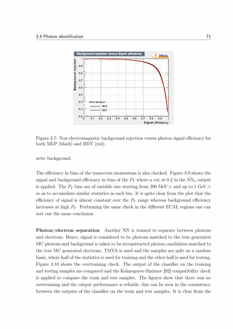
3.4 Photon identification 71
Figure 3.7: Non electromagnetic background rejection versus photon signal efficiency forboth MLP (black) and BDT (red).
netic background.
The efficiency in bins of the transverse momentum is also checked. Figure 3.9 shows thesignal and background efficiency in bins of the PT where a cut at 0.2 in the NNh outputis applied. The PT bins are of variable size starting from 200 MeV/c and up to 1 GeV/cso as to accumulate similar statistics in each bin. It is quite clear from the plot that theefficiency of signal is almost constant over the PT range whereas background efficiencyincreases at high PT . Performing the same check in the different ECAL regions one cansort out the same conclusion.
Photon/electron separation Another NN is trained to separate between photonsand electrons. Hence, signal is considered to be photons matched to the true generatedMC photons and background is taken to be reconstructed photon candidates matched tothe true MC generated electrons. TMVA is used and the samples are split on a randombasis, where half of the statistics is used for training and the other half is used for testing.Figure 3.10 shows the overtraining check. The output of the classifier on the trainingand testing samples are compared and the Kolmogorov-Smirnov [92] compatibility checkis applied to compare the train and test samples. The figures show that there was noovertraining and the output performance is reliable, this can be seen in the consistencybetween the outputs of the classifier on the train and test samples. It is clear from the
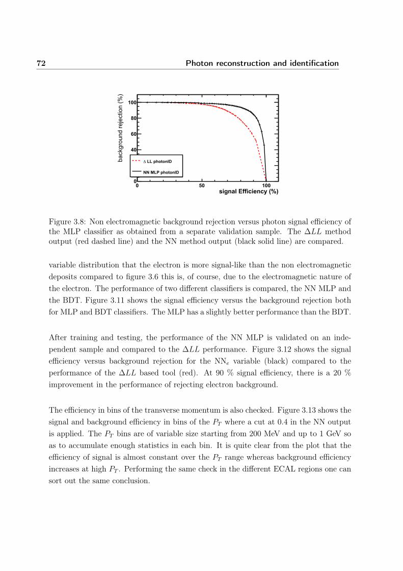
72 Photon reconstruction and identification
������������� ����� �� ���
��� ����� �����������
�
��
��
��
��
���
�������������Δ
��� �!���������
Figure 3.8: Non electromagnetic background rejection versus photon signal efficiency ofthe MLP classifier as obtained from a separate validation sample. The ΔLL methodoutput (red dashed line) and the NN method output (black solid line) are compared.
variable distribution that the electron is more signal-like than the non electromagneticdeposits compared to figure 3.6 this is, of course, due to the electromagnetic nature ofthe electron. The performance of two different classifiers is compared, the NN MLP andthe BDT. Figure 3.11 shows the signal efficiency versus the background rejection bothfor MLP and BDT classifiers. The MLP has a slightly better performance than the BDT.
After training and testing, the performance of the NN MLP is validated on an inde-pendent sample and compared to the ΔLL performance. Figure 3.12 shows the signalefficiency versus background rejection for the NNe variable (black) compared to theperformance of the ΔLL based tool (red). At 90 % signal efficiency, there is a 20 %improvement in the performance of rejecting electron background.
The efficiency in bins of the transverse momentum is also checked. Figure 3.13 shows thesignal and background efficiency in bins of the PT where a cut at 0.4 in the NN outputis applied. The PT bins are of variable size starting from 200 MeV and up to 1 GeV soas to accumulate enough statistics in each bin. It is quite clear from the plot that theefficiency of signal is almost constant over the PT range whereas background efficiencyincreases at high PT . Performing the same check in the different ECAL regions one cansort out the same conclusion.
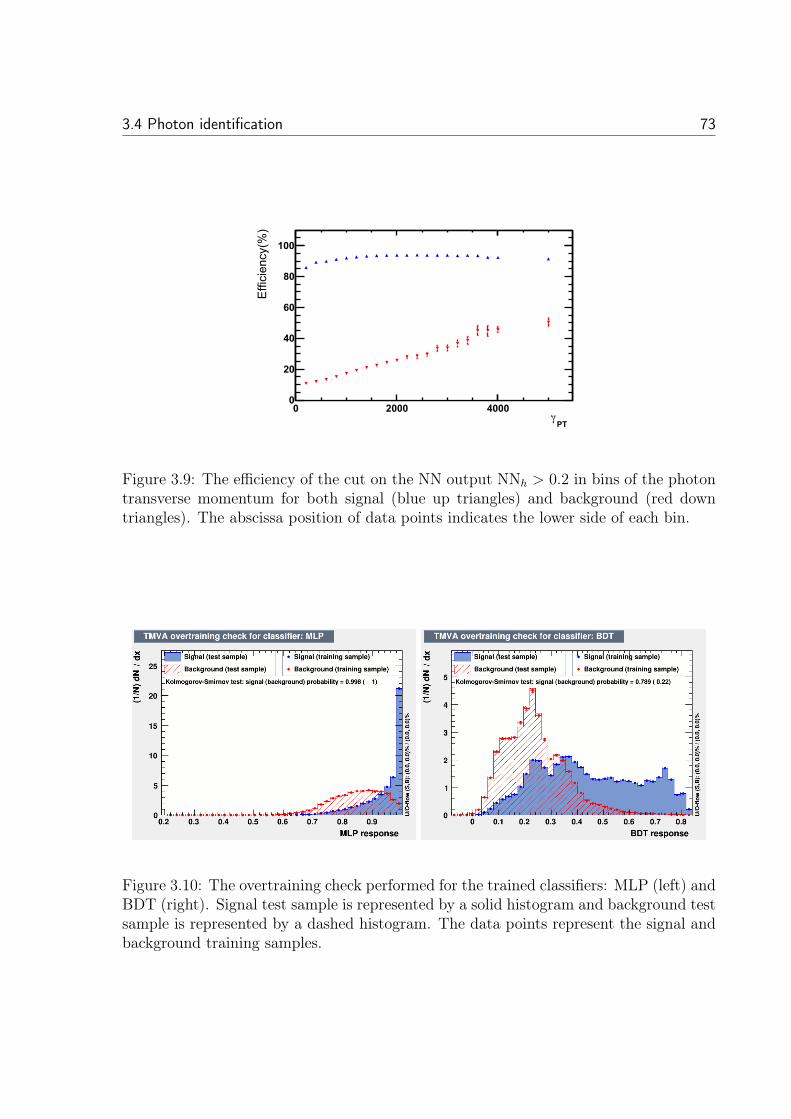
3.4 Photon identification 73
�!"γ
� ���� ����
�����������
�
��
��
��
��
���
Figure 3.9: The efficiency of the cut on the NN output NNh > 0.2 in bins of the photontransverse momentum for both signal (blue up triangles) and background (red downtriangles). The abscissa position of data points indicates the lower side of each bin.
Figure 3.10: The overtraining check performed for the trained classifiers: MLP (left) andBDT (right). Signal test sample is represented by a solid histogram and background testsample is represented by a dashed histogram. The data points represent the signal andbackground training samples.
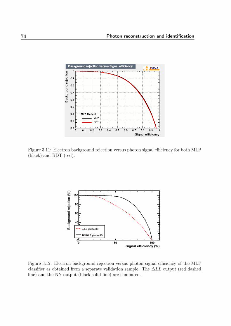
74 Photon reconstruction and identification
Figure 3.11: Electron background rejection versus photon signal efficiency for both MLP(black) and BDT (red).
#������������� ����� �� ���
���� ����� �����������
�
��
��
��
��
���
�������������Δ
��� �!���������
Figure 3.12: Electron background rejection versus photon signal efficiency of the MLPclassifier as obtained from a separate validation sample. The ΔLL output (red dashedline) and the NN output (black solid line) are compared.
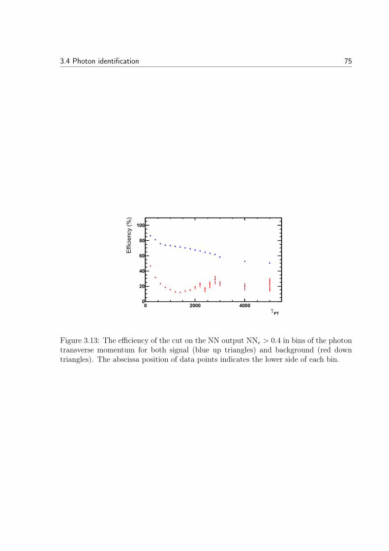
3.4 Photon identification 75
�!"γ
� ���� ����
������������
�
��
��
��
��
���
Figure 3.13: The efficiency of the cut on the NN output NNe > 0.4 in bins of the photontransverse momentum for both signal (blue up triangles) and background (red downtriangles). The abscissa position of data points indicates the lower side of each bin.
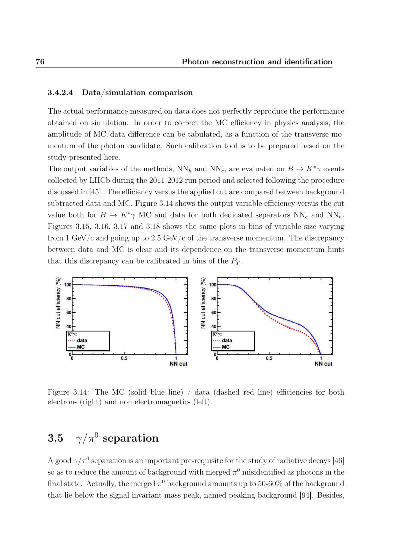
76 Photon reconstruction and identification
3.4.2.4 Data/simulation comparison
The actual performance measured on data does not perfectly reproduce the performanceobtained on simulation. In order to correct the MC efficiency in physics analysis, theamplitude of MC/data difference can be tabulated, as a function of the transverse mo-mentum of the photon candidate. Such calibration tool is to be prepared based on thestudy presented here.The output variables of the methods, NNh and NNe, are evaluated on B → K∗γ eventscollected by LHCb during the 2011-2012 run period and selected following the procedurediscussed in [45]. The efficiency versus the applied cut are compared between backgroundsubtracted data and MC. Figure 3.14 shows the output variable efficiency versus the cutvalue both for B → K∗γ MC and data for both dedicated separators NNe and NNh.Figures 3.15, 3.16, 3.17 and 3.18 shows the same plots in bins of variable size varyingfrom 1 GeV/c and going up to 2.5 GeV/c of the transverse momentum. The discrepancybetween data and MC is clear and its dependence on the transverse momentum hintsthat this discrepancy can be calibrated in bins of the PT .
Figure 3.14: The MC (solid blue line) / data (dashed red line) efficiencies for bothelectron- (right) and non electromagnetic- (left).
3.5 γ/π0 separation
A good γ/π0 separation is an important pre-requisite for the study of radiative decays [46]so as to reduce the amount of background with merged π0 misidentified as photons in thefinal state. Actually, the merged π0 background amounts up to 50-60% of the backgroundthat lie below the signal invariant mass peak, named peaking background [94]. Besides,
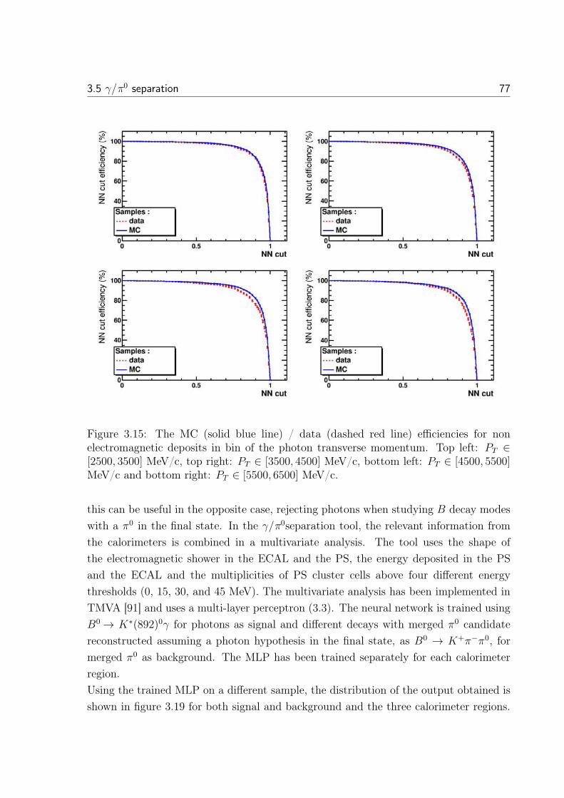
3.5 γ/π0 separation 77
Figure 3.15: The MC (solid blue line) / data (dashed red line) efficiencies for nonelectromagnetic deposits in bin of the photon transverse momentum. Top left: PT ∈[2500, 3500] MeV/c, top right: PT ∈ [3500, 4500] MeV/c, bottom left: PT ∈ [4500, 5500]MeV/c and bottom right: PT ∈ [5500, 6500] MeV/c.
this can be useful in the opposite case, rejecting photons when studying B decay modeswith a π0 in the final state. In the γ/π0separation tool, the relevant information fromthe calorimeters is combined in a multivariate analysis. The tool uses the shape ofthe electromagnetic shower in the ECAL and the PS, the energy deposited in the PSand the ECAL and the multiplicities of PS cluster cells above four different energythresholds (0, 15, 30, and 45 MeV). The multivariate analysis has been implemented inTMVA [91] and uses a multi-layer perceptron (3.3). The neural network is trained usingB0 → K∗(892)0γ for photons as signal and different decays with merged π0 candidatereconstructed assuming a photon hypothesis in the final state, as B0 → K+π−π0, formerged π0 as background. The MLP has been trained separately for each calorimeterregion.Using the trained MLP on a different sample, the distribution of the output obtained isshown in figure 3.19 for both signal and background and the three calorimeter regions.
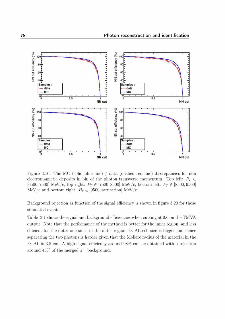
78 Photon reconstruction and identification
Figure 3.16: The MC (solid blue line) / data (dashed red line) discrepancies for nonelectromagnetic deposits in bin of the photon transverse momentum. Top left: PT ∈[6500, 7500] MeV/c, top right: PT ∈ [7500, 8500] MeV/c, bottom left: PT ∈ [8500, 9500]MeV/c and bottom right: PT ∈ [9500, saturation] MeV/c.
Background rejection as function of the signal efficiency is shown in figure 3.20 for thosesimulated events.
Table 3.1 shows the signal and background efficiencies when cutting at 0.6 on the TMVAoutput. Note that the performance of the method is better for the inner region, and lessefficient for the outer one since in the outer region, ECAL cell size is bigger and henceseparating the two photons is harder given that the Moliere radius of the material in theECAL is 3.5 cm. A high signal efficiency around 98% can be obtained with a rejectionaround 45% of the merged π0 background.
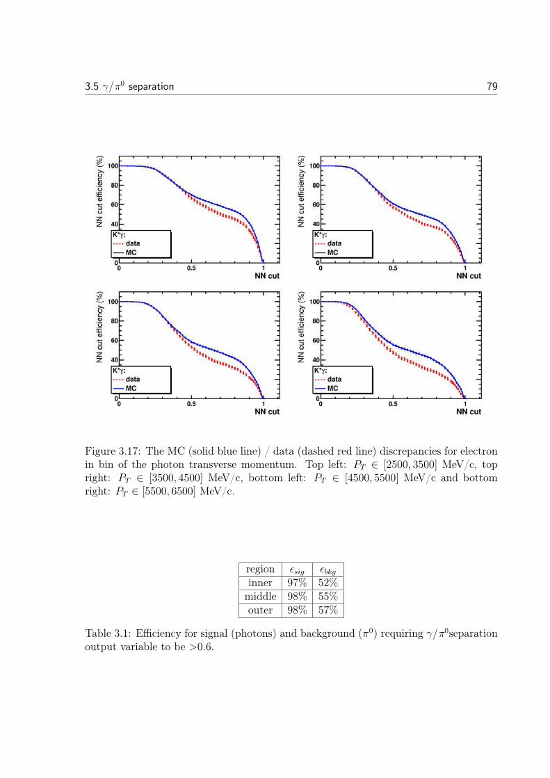
3.5 γ/π0 separation 79
Figure 3.17: The MC (solid blue line) / data (dashed red line) discrepancies for electronin bin of the photon transverse momentum. Top left: PT ∈ [2500, 3500] MeV/c, topright: PT ∈ [3500, 4500] MeV/c, bottom left: PT ∈ [4500, 5500] MeV/c and bottomright: PT ∈ [5500, 6500] MeV/c.
region εsig εbkginner 97% 52%
middle 98% 55%outer 98% 57%
Table 3.1: Efficiency for signal (photons) and background (π0) requiring γ/π0separationoutput variable to be >0.6.
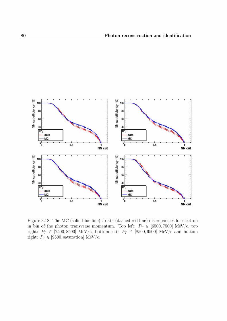
80 Photon reconstruction and identification
Figure 3.18: The MC (solid blue line) / data (dashed red line) discrepancies for electronin bin of the photon transverse momentum. Top left: PT ∈ [6500, 7500] MeV/c, topright: PT ∈ [7500, 8500] MeV/c, bottom left: PT ∈ [8500, 9500] MeV/c and bottomright: PT ∈ [9500, saturation] MeV/c.
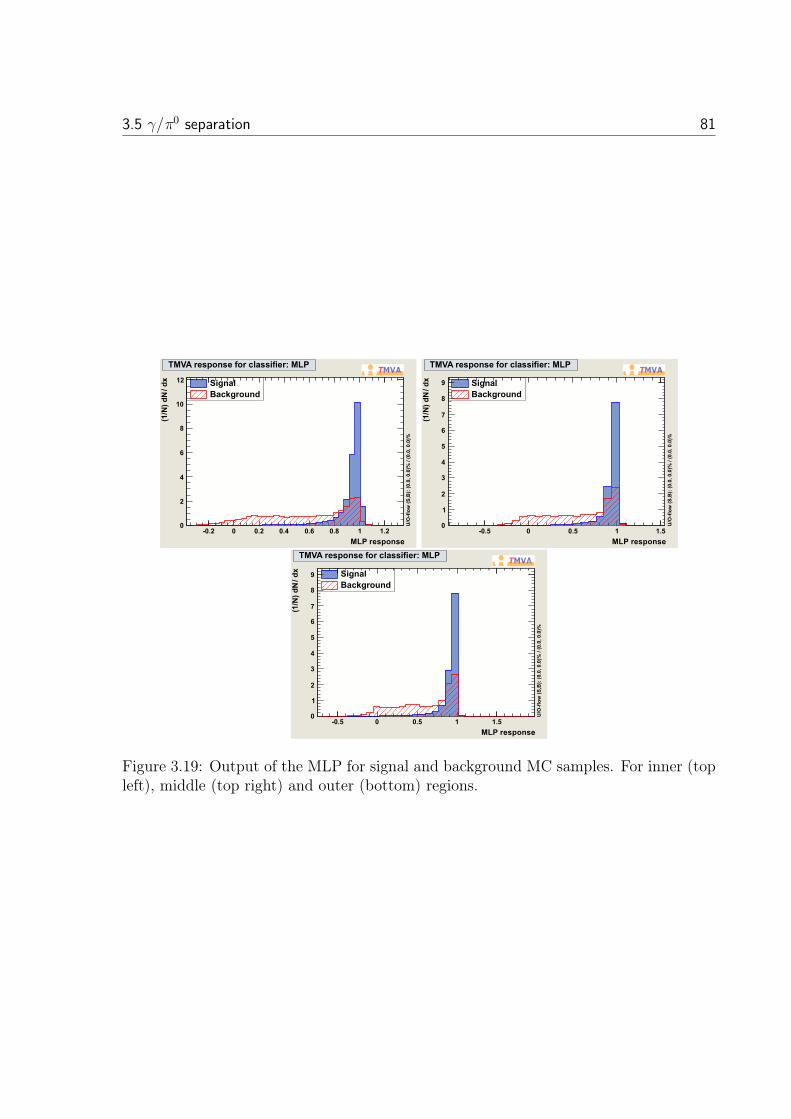
3.5 γ/π0 separation 81
�!�$�������%�&� � �&� �&� �&� �&� � �&�
'(� )���)���'�
�
�
�
�
�
��
�� #�����*��+�$�,�'
-).%��/��#0*�1���&�0��&����)���&�0��&���
" 23�$���������$���������$1� �!
�!�$�������%�&� � �&� � �&�
'(� )���)���'�
�
�
�
4
�
�
�
5
�
6 #�����*��+�$�,�'
-).%��/��#0*�1���&�0��&����)���&�0��&���
" 23�$���������$���������$1� �!
�!�$�������%�&� � �&� � �&�
'(� )���)���'�
�
�
�
4
�
�
�
5
�
6 #�����*��+�$�,�'
-).%��/��#0*�1���&�0��&����)���&�0��&���
" 23�$���������$���������$1� �!
Figure 3.19: Output of the MLP for signal and background MC samples. For inner (topleft), middle (top right) and outer (bottom) regions.
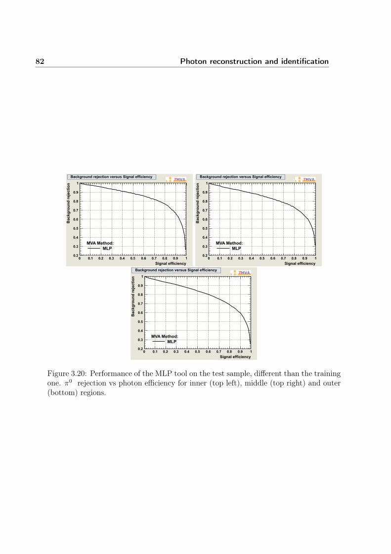
82 Photon reconstruction and identification
#������������� � �&� �&� �&4 �&� �&� �&� �&5 �&� �&6 �
*��+�$�,�'�$�7������
�&�
�&4
�&�
�&�
�&�
�&5
�&�
�&6
�
23� ����'1 �!
*��+�$�,�'�$�7�������8�$�,��#�������������
#������������� � �&� �&� �&4 �&� �&� �&� �&5 �&� �&6 �
*��+�$�,�'�$�7������
�&�
�&4
�&�
�&�
�&�
�&5
�&�
�&6
�
23� ����'1 �!
*��+�$�,�'�$�7�������8�$�,��#�������������
#������������� � �&� �&� �&4 �&� �&� �&� �&5 �&� �&6 �
*��+�$�,�'�$�7������
�&�
�&4
�&�
�&�
�&�
�&5
�&�
�&6
�
23� ����'1 �!
*��+�$�,�'�$�7�������8�$�,��#�������������
Figure 3.20: Performance of the MLP tool on the test sample, different than the trainingone. π0 rejection vs photon efficiency for inner (top left), middle (top right) and outer(bottom) regions.
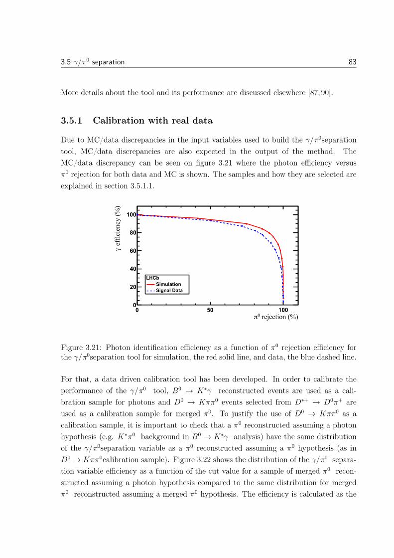
3.5 γ/π0 separation 83
More details about the tool and its performance are discussed elsewhere [87,90].
3.5.1 Calibration with real data
Due to MC/data discrepancies in the input variables used to build the γ/π0separationtool, MC/data discrepancies are also expected in the output of the method. TheMC/data discrepancy can be seen on figure 3.21 where the photon efficiency versusπ0 rejection for both data and MC is shown. The samples and how they are selected areexplained in section 3.5.1.1.
�� � ����������π� �� ���
� ����� �������
γ
�
��
��
��
��
���
�9:;#�<,�������#����������
Figure 3.21: Photon identification efficiency as a function of π0 rejection efficiency forthe γ/π0separation tool for simulation, the red solid line, and data, the blue dashed line.
For that, a data driven calibration tool has been developed. In order to calibrate theperformance of the γ/π0 tool, B0 → K∗γ reconstructed events are used as a cali-bration sample for photons and D0 → Kππ0 events selected from D∗+ → D0π+ areused as a calibration sample for merged π0. To justify the use of D0 → Kππ0 as acalibration sample, it is important to check that a π0 reconstructed assuming a photonhypothesis (e.g. K∗π0 background in B0 → K∗γ analysis) have the same distributionof the γ/π0separation variable as a π0 reconstructed assuming a π0 hypothesis (as inD0 → Kππ0calibration sample). Figure 3.22 shows the distribution of the γ/π0 separa-tion variable efficiency as a function of the cut value for a sample of merged π0 recon-structed assuming a photon hypothesis compared to the same distribution for mergedπ0 reconstructed assuming a merged π0 hypothesis. The efficiency is calculated as the
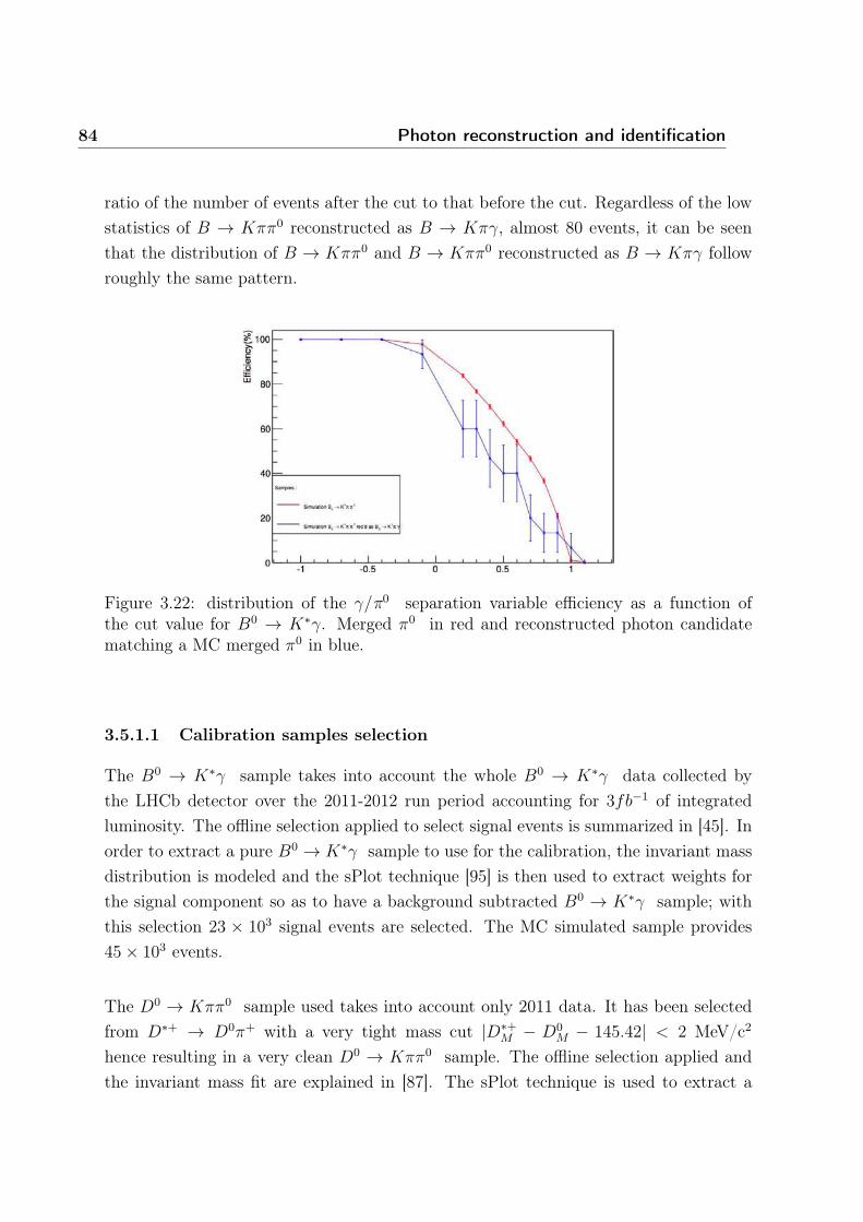
84 Photon reconstruction and identification
ratio of the number of events after the cut to that before the cut. Regardless of the lowstatistics of B → Kππ0 reconstructed as B → Kπγ, almost 80 events, it can be seenthat the distribution of B → Kππ0 and B → Kππ0 reconstructed as B → Kπγ followroughly the same pattern.
Figure 3.22: distribution of the γ/π0 separation variable efficiency as a function ofthe cut value for B0 → K∗γ. Merged π0 in red and reconstructed photon candidatematching a MC merged π0 in blue.
3.5.1.1 Calibration samples selection
The B0 → K∗γ sample takes into account the whole B0 → K∗γ data collected bythe LHCb detector over the 2011-2012 run period accounting for 3fb−1 of integratedluminosity. The offline selection applied to select signal events is summarized in [45]. Inorder to extract a pure B0 → K∗γ sample to use for the calibration, the invariant massdistribution is modeled and the sPlot technique [95] is then used to extract weights forthe signal component so as to have a background subtracted B0 → K∗γ sample; withthis selection 23 × 103 signal events are selected. The MC simulated sample provides45× 103 events.
The D0 → Kππ0 sample used takes into account only 2011 data. It has been selectedfrom D∗+ → D0π+ with a very tight mass cut |D∗+
M − D0M − 145.42| < 2 MeV/c2
hence resulting in a very clean D0 → Kππ0 sample. The offline selection applied andthe invariant mass fit are explained in [87]. The sPlot technique is used to extract a
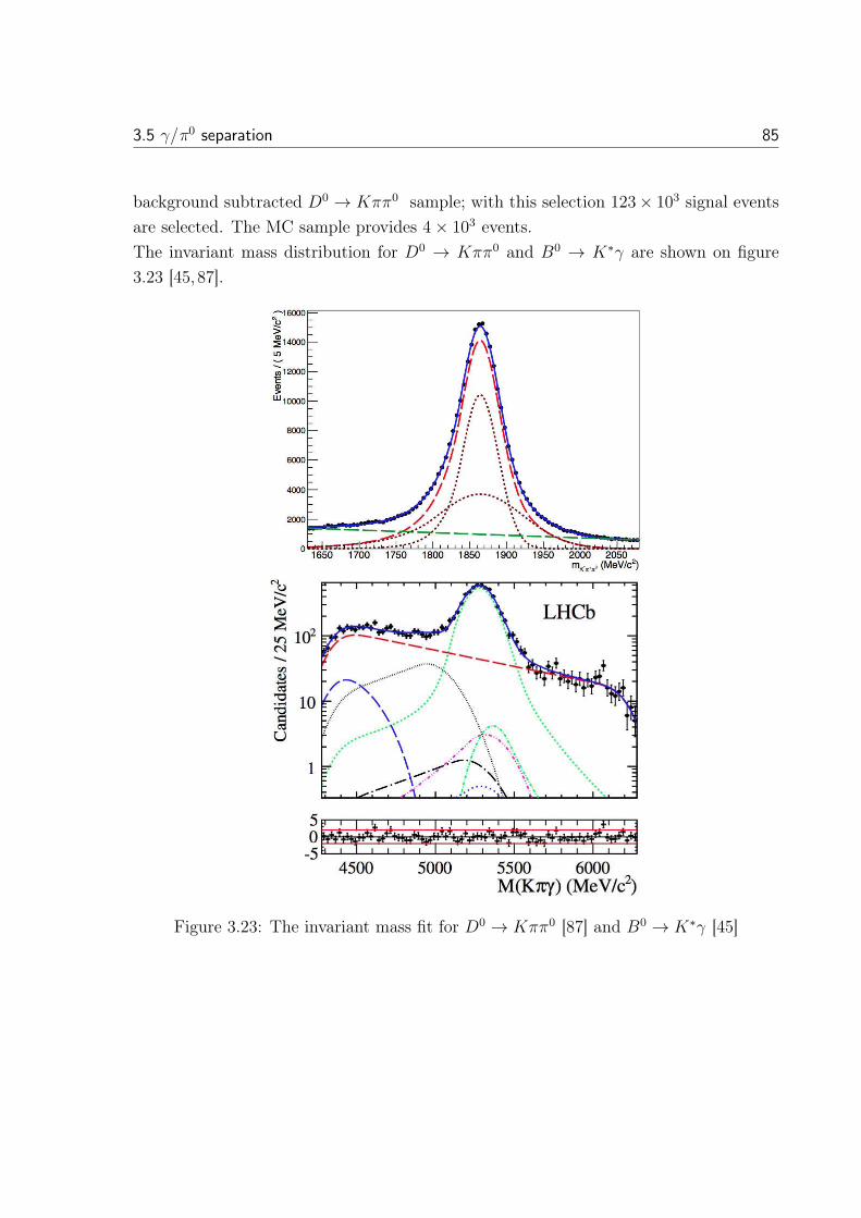
3.5 γ/π0 separation 85
background subtracted D0 → Kππ0 sample; with this selection 123× 103 signal eventsare selected. The MC sample provides 4× 10³ events.The invariant mass distribution for D0 → Kππ0 and B0 → K∗γ are shown on figure3.23 [45,87].
Figure 3.23: The invariant mass fit for D0 → Kππ0 [87] and B0 → K∗γ [45]
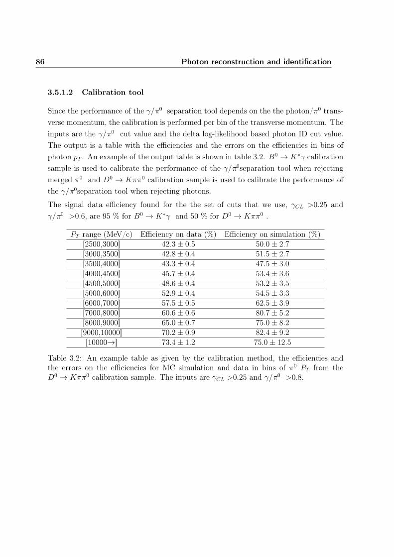
86 Photon reconstruction and identification
3.5.1.2 Calibration tool
Since the performance of the γ/π0 separation tool depends on the the photon/π0 trans-verse momentum, the calibration is performed per bin of the transverse momentum. Theinputs are the γ/π0 cut value and the delta log-likelihood based photon ID cut value.The output is a table with the efficiencies and the errors on the efficiencies in bins ofphoton pT . An example of the output table is shown in table 3.2. B0 → K∗γ calibrationsample is used to calibrate the performance of the γ/π0separation tool when rejectingmerged π0 and D0 → Kππ0 calibration sample is used to calibrate the performance ofthe γ/π0separation tool when rejecting photons.
The signal data efficiency found for the the set of cuts that we use, γCL >0.25 andγ/π0 >0.6, are 95 % for B0 → K∗γ and 50 % for D0 → Kππ0 .
PT range (MeV/c) Efficiency on data (%) Efficiency on simulation (%)[2500,3000] 42.3± 0.5 50.0± 2.7[3000,3500] 42.8± 0.4 51.5± 2.7[3500,4000] 43.3± 0.4 47.5± 3.0[4000,4500] 45.7± 0.4 53.4± 3.6[4500,5000] 48.6± 0.4 53.2± 3.5[5000,6000] 52.9± 0.4 54.5± 3.3[6000,7000] 57.5± 0.5 62.5± 3.9[7000,8000] 60.6± 0.6 80.7± 5.2[8000,9000] 65.0± 0.7 75.0± 8.2[9000,10000] 70.2± 0.9 82.4± 9.2[10000→] 73.4± 1.2 75.0± 12.5
Table 3.2: An example table as given by the calibration method, the efficiencies andthe errors on the efficiencies for MC simulation and data in bins of π0 PT from theD0 → Kππ0 calibration sample. The inputs are γCL >0.25 and γ/π0 >0.8.
Chapter 4
The measurement of the photonpolarization in B0
s→ φγ
Contents4.1 Introduction . . . . . . . . . . . . . . . . . . . . . . . . . . . . 88
4.2 Signal and control channels selection . . . . . . . . . . . . . . 91
4.2.1 Trigger . . . . . . . . . . . . . . . . . . . . . . . . . . . . . . . . 91
4.2.2 Signal reconstruction and selection . . . . . . . . . . . . . . . . 93
4.2.3 Mass models and background subtraction . . . . . . . . . . . . 95
4.3 The proper time . . . . . . . . . . . . . . . . . . . . . . . . . . 102
4.3.1 The proper time reconstruction . . . . . . . . . . . . . . . . . . 102
4.3.2 Proper time distribution model for signal . . . . . . . . . . . . 103
4.4 Proper time acceptance study on MC . . . . . . . . . . . . . 113
4.4.1 Acceptance at low proper time, B0→ J/ψX weighing and cutscaling procedure. . . . . . . . . . . . . . . . . . . . . . . . . . 113
4.4.2 Proper time in simulated data . . . . . . . . . . . . . . . . . . . 117
4.4.3 Acceptance at high proper time introduced by the trigger . . . 124
4.4.4 Proper time distribution of control samples in data . . . . . . . 125
4.4.5 Measurement strategies . . . . . . . . . . . . . . . . . . . . . . 127
87
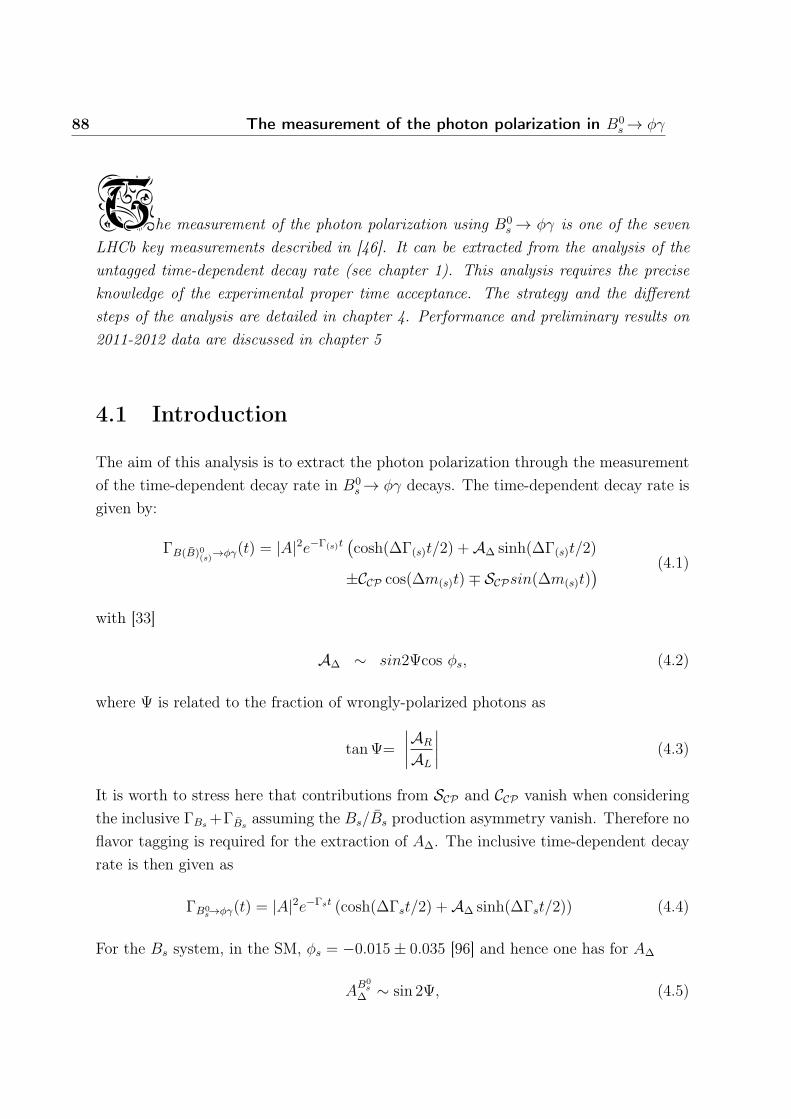
88 The measurement of the photon polarization in B0s → φγ
The measurement of the photon polarization using B0s → φγ is one of the seven
LHCb key measurements described in [46]. It can be extracted from the analysis of theuntagged time-dependent decay rate (see chapter 1). This analysis requires the preciseknowledge of the experimental proper time acceptance. The strategy and the differentsteps of the analysis are detailed in chapter 4. Performance and preliminary results on2011-2012 data are discussed in chapter 5
4.1 Introduction
The aim of this analysis is to extract the photon polarization through the measurementof the time-dependent decay rate in B0
s → φγ decays. The time-dependent decay rate isgiven by:
ΓB(B)0(s)
→φγ(t) = |A|2e−Γ(s)t(cosh(ΔΓ(s)t/2) +AΔ sinh(ΔΓ(s)t/2)
±CCP cos(Δm(s)t)∓ SCPsin(Δm(s)t)) (4.1)
with [33]
AΔ ∼ sin2Ψcos φs, (4.2)
where Ψ is related to the fraction of wrongly-polarized photons as
tanΨ=
∣∣∣∣AR
AL
∣∣∣∣ (4.3)
It is worth to stress here that contributions from SCP and CCP vanish when consideringthe inclusive ΓBs+ΓBs
assuming the Bs/Bs production asymmetry vanish. Therefore noflavor tagging is required for the extraction of AΔ. The inclusive time-dependent decayrate is then given as
ΓB0s→φγ(t) = |A|2e−Γst (cosh(ΔΓst/2) +AΔ sinh(ΔΓst/2)) (4.4)
For the Bs system, in the SM, φs = −0.015± 0.035 [96] and hence one has for AΔ
AB0
sΔ ∼ sin 2Ψ, (4.5)
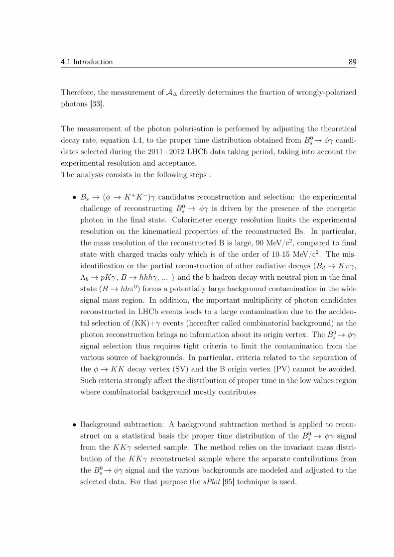
4.1 Introduction 89
Therefore, the measurement of AΔ directly determines the fraction of wrongly-polarizedphotons [33].
The measurement of the photon polarisation is performed by adjusting the theoreticaldecay rate, equation 4.4, to the proper time distribution obtained from B0
s → φγ candi-dates selected during the 2011+2012 LHCb data taking period, taking into account theexperimental resolution and acceptance.The analysis consists in the following steps :
• Bs → (φ → K+K−)γ candidates reconstruction and selection: the experimentalchallenge of reconstructing B0
s → φγ is driven by the presence of the energeticphoton in the final state. Calorimeter energy resolution limits the experimentalresolution on the kinematical properties of the reconstructed Bs. In particular,the mass resolution of the reconstructed B is large, 90 MeV/c2, compared to finalstate with charged tracks only which is of the order of 10-15 MeV/c2. The mis-identification or the partial reconstruction of other radiative decays (Bd → Kπγ,Λb → pKγ , B → hhhγ, ... ) and the b-hadron decay with neutral pion in the finalstate (B → hhπ0) forms a potentially large background contamination in the widesignal mass region. In addition, the important multiplicity of photon candidatesreconstructed in LHCb events leads to a large contamination due to the acciden-tal selection of (KK)+γ events (hereafter called combinatorial background) as thephoton reconstruction brings no information about its origin vertex. The B0
s → φγ
signal selection thus requires tight criteria to limit the contamination from thevarious source of backgrounds. In particular, criteria related to the separation ofthe φ → KK decay vertex (SV) and the B origin vertex (PV) cannot be avoided.Such criteria strongly affect the distribution of proper time in the low values regionwhere combinatorial background mostly contributes.
• Background subtraction: A background subtraction method is applied to recon-struct on a statistical basis the proper time distribution of the B0
s → φγ signalfrom the KKγ selected sample. The method relies on the invariant mass distri-bution of the KKγ reconstructed sample where the separate contributions fromthe B0
s → φγ signal and the various backgrounds are modeled and adjusted to theselected data. For that purpose the sPlot [95] technique is used.
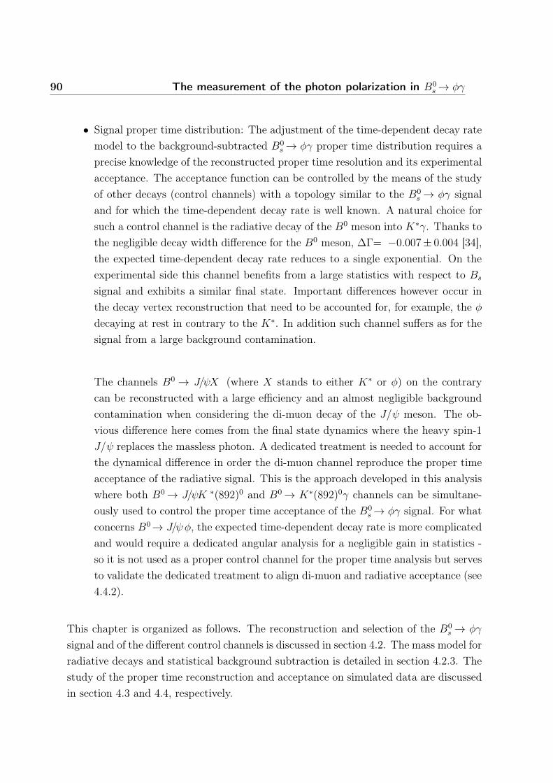
90 The measurement of the photon polarization in B0s → φγ
• Signal proper time distribution: The adjustment of the time-dependent decay ratemodel to the background-subtracted B0
s → φγ proper time distribution requires aprecise knowledge of the reconstructed proper time resolution and its experimentalacceptance. The acceptance function can be controlled by the means of the studyof other decays (control channels) with a topology similar to the B0
s → φγ signaland for which the time-dependent decay rate is well known. A natural choice forsuch a control channel is the radiative decay of the B0 meson into K∗γ. Thanks tothe negligible decay width difference for the B0 meson, ΔΓ= −0.007± 0.004 [34],the expected time-dependent decay rate reduces to a single exponential. On theexperimental side this channel benefits from a large statistics with respect to Bs
signal and exhibits a similar final state. Important differences however occur inthe decay vertex reconstruction that need to be accounted for, for example, the φ
decaying at rest in contrary to the K∗. In addition such channel suffers as for thesignal from a large background contamination.
The channels B0 → J/ψX (where X stands to either K∗ or φ) on the contrarycan be reconstructed with a large efficiency and an almost negligible backgroundcontamination when considering the di-muon decay of the J/ψ meson. The ob-vious difference here comes from the final state dynamics where the heavy spin-1J/ψ replaces the massless photon. A dedicated treatment is needed to account forthe dynamical difference in order the di-muon channel reproduce the proper timeacceptance of the radiative signal. This is the approach developed in this analysiswhere both B0 → J/ψK ∗(892)0 and B0 → K∗(892)0γ channels can be simultane-ously used to control the proper time acceptance of the B0
s → φγ signal. For whatconcerns B0→ J/ψφ, the expected time-dependent decay rate is more complicatedand would require a dedicated angular analysis for a negligible gain in statistics -so it is not used as a proper control channel for the proper time analysis but servesto validate the dedicated treatment to align di-muon and radiative acceptance (see4.4.2).
This chapter is organized as follows. The reconstruction and selection of the B0s → φγ
signal and of the different control channels is discussed in section 4.2. The mass model forradiative decays and statistical background subtraction is detailed in section 4.2.3. Thestudy of the proper time reconstruction and acceptance on simulated data are discussedin section 4.3 and 4.4, respectively.
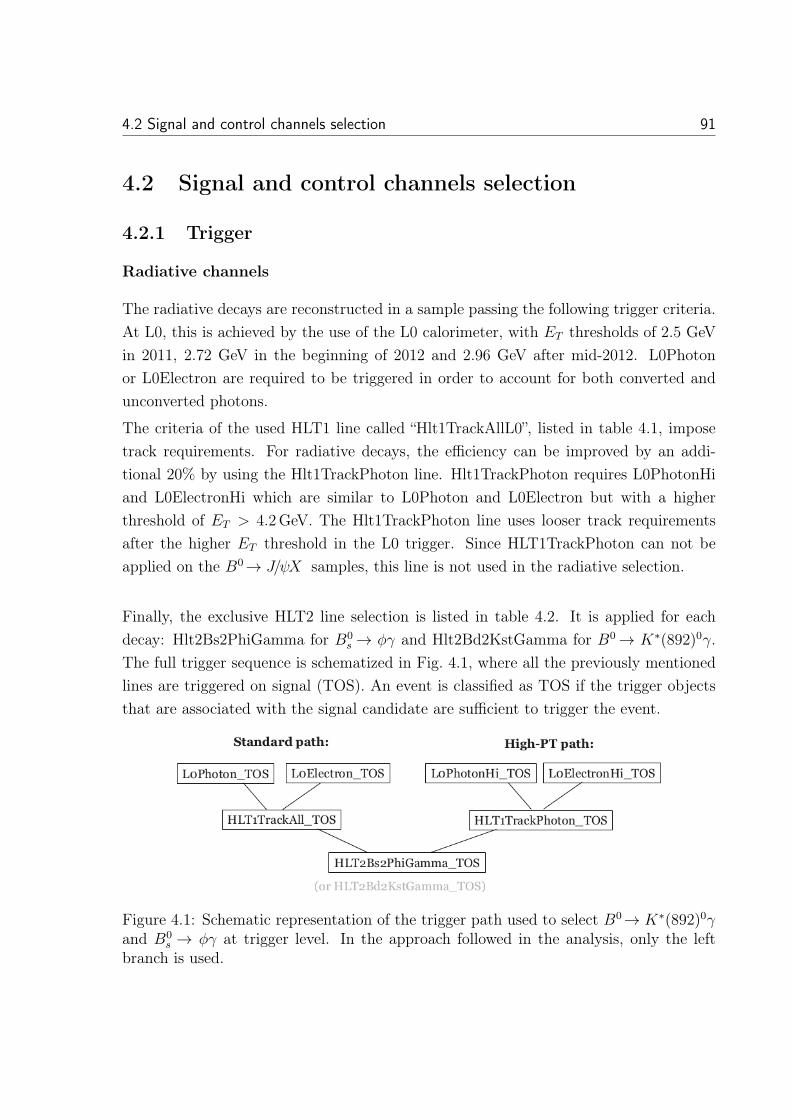
4.2 Signal and control channels selection 91
4.2 Signal and control channels selection
4.2.1 Trigger
Radiative channels
The radiative decays are reconstructed in a sample passing the following trigger criteria.At L0, this is achieved by the use of the L0 calorimeter, with ET thresholds of 2.5 GeVin 2011, 2.72 GeV in the beginning of 2012 and 2.96 GeV after mid-2012. L0Photonor L0Electron are required to be triggered in order to account for both converted andunconverted photons.
The criteria of the used HLT1 line called “Hlt1TrackAllL0”, listed in table 4.1, imposetrack requirements. For radiative decays, the efficiency can be improved by an addi-tional 20% by using the Hlt1TrackPhoton line. Hlt1TrackPhoton requires L0PhotonHiand L0ElectronHi which are similar to L0Photon and L0Electron but with a higherthreshold of ET > 4.2GeV. The Hlt1TrackPhoton line uses looser track requirementsafter the higher ET threshold in the L0 trigger. Since HLT1TrackPhoton can not beapplied on the B0→ J/ψX samples, this line is not used in the radiative selection.
Finally, the exclusive HLT2 line selection is listed in table 4.2. It is applied for eachdecay: Hlt2Bs2PhiGamma for B0
s → φγ and Hlt2Bd2KstGamma for B0 → K∗(892)0γ.The full trigger sequence is schematized in Fig. 4.1, where all the previously mentionedlines are triggered on signal (TOS). An event is classified as TOS if the trigger objectsthat are associated with the signal candidate are sufficient to trigger the event.
Figure 4.1: Schematic representation of the trigger path used to select B0→ K∗(892)0γand B0
s → φγ at trigger level. In the approach followed in the analysis, only the leftbranch is used.
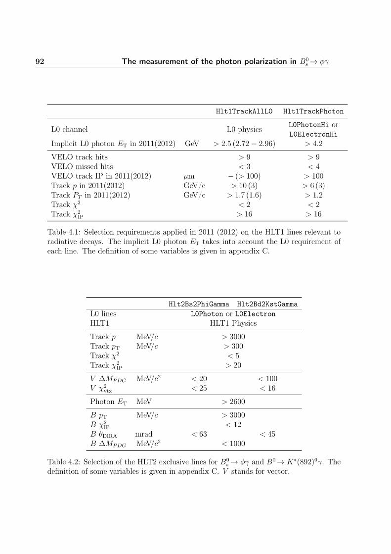
92 The measurement of the photon polarization in B0s → φγ
Hlt1TrackAllL0 Hlt1TrackPhoton
L0 channel L0 physics L0PhotonHi orL0ElectronHi
Implicit L0 photon ET in 2011(2012) GeV > 2.5 (2.72− 2.96) > 4.2
VELO track hits > 9 > 9VELO missed hits < 3 < 4VELO track IP in 2011(2012) μm − (> 100) > 100Track p in 2011(2012) GeV/c > 10 (3) > 6 (3)Track PT in 2011(2012) GeV/c > 1.7 (1.6) > 1.2Track χ2 < 2 < 2Track χ2
IP > 16 > 16
Table 4.1: Selection requirements applied in 2011 (2012) on the HLT1 lines relevant toradiative decays. The implicit L0 photon ET takes into account the L0 requirement ofeach line. The definition of some variables is given in appendix C.
Hlt2Bs2PhiGamma Hlt2Bd2KstGammaL0 lines L0Photon or L0ElectronHLT1 HLT1 Physics
Track p MeV/c > 3000Track pT MeV/c > 300Track χ2 < 5Track χ2
IP > 20
V ΔMPDG MeV/c2 < 20 < 100V χ2
vtx < 25 < 16
Photon ET MeV > 2600
B pT MeV/c > 3000B χ2
IP < 12B θDIRA mrad < 63 < 45B ΔMPDG MeV/c2 < 1000
Table 4.2: Selection of the HLT2 exclusive lines for B0s → φγ and B0→ K∗(892)0γ. The
definition of some variables is given in appendix C. V stands for vector.
4.2 Signal and control channels selection 93
Dimuon channels
The trigger path chosen for the B0 → J/ψX candidates is based on the muon trigger.This trigger path is proper time unbiased since it contains no explicit cuts on variablesthat induce a proper time acceptance. Nevertheless, residual bias in the proper time isobserved and discussed in details in section 4.4.3. The trigger path is
• The L0 trigger used is L0Muon or L0DiMuon.
• In HLT1, the Hlt1DiMuonHighMass line is used, with a further TOS requirementon HLT1TrackAllL0 to align the selection to the radiative one. As will be shownin Section 4.4.3, only the HLT1 has an impact on the acceptance at high propertime relatively to the offline selection.
• In HLT2, the Hlt2DiMuonJPsiHighPT line is used.
4.2.2 Signal reconstruction and selection
At LHCb, the excellent vertex resolution of the VELO and the large boost of the Bhadrons produced at the LHC makes possible to distinguish the primary vertex (PV),where the b-hadron is produced, from the secondary vertex (SV) where its decay takesplace. Moreover, the high mass of the B mesons drives the kinematics of the decay andhence, most of the mass of the B is transformed in kinetic energy of the decay productswhich tend to scatter with large angles with respect to the direction of flight of the B.As a result, the B decay products have high transverse momenta.
For radiative decays as Bs → (φ → K+K−)γ and B0 → (K∗(892)0 → K+π−)γ, thefinal state consists of two tracks and a photon. To reconstruct such decays one looks fortwo tracks that form a well separated SV. The B candidate is associated with a PV ona geometrical basis requiring the angle between the reconstructed B momentum and theline connecting the PV and the SV to be small. Require that the particles associated tothe selected tracks are of opposite charges and of high transverse momentum. Finally,the energy of the photon is reconstructed relying on the calorimeter. The invariant massof the three body final state, i.e. the two hadrons and the photon, is required to be inthe ±1GeV/c2 range around the nominal B mass value.
For the selection of B0 → (J/ψ → μ+μ−)(K∗(892)0 → K+π−) and Bs → (J/ψ →μ+μ−)(φ → K+K−) decays, similar criteria is applied. Performing tracks selection, SV

94 The measurement of the photon polarization in B0s → φγ
reconstruction, associating the reconstructed B hadron to the PV and applying PID andPT cuts to select the desired particles.
The di-muon channels B0→ J/ψK ∗(892)0 and B0s → J/ψφ are used as control samples
for the proper time acceptance. For this to be possible, and since the di-muon and ra-diative channels have the same hadronic part, the J/ψ in the di-muon channels shouldmimic the behavior of the photon in radiative decays. This is achieved by excludingthe di-muon system from the B decay vertex reconstruction by increasing the covariancematrix element associated to the di-muon tracks to a very high value at which they nolonger participate in the vertex computation of the B.
The main selection criteria are
• The two tracks are required to be of good quality. It can be tested looking at theχ2/ndof of the track fit.
• The two tracks do not come from a PV, meaning that the impact parameter (IP)- being the shortest distance from the track to the PV - of their trajectories withrespect to any PV has to be large.
• The two tracks form a secondary vertex. The χ2 of the vertex fit is required to besmall.
• The B meson comes from a PV. Its reconstructed IP is required to be small withrespect to this point.
• The direction of flight of the B from the primary to the secondary vertices shouldmatch the direction of the momentum of the B, obtained as the vector sum of themomentum of the final particles. The matching is measured by the angle betweenthe direction of flight of the B and the direction of the momentum of the B, θDIRA.θDIRA is required to be small.
• The transverse momentum (PT ) of the decay daughters is high.
• The invariant mass of the reconstructed decay final state is required to be in the±1GeV/c2 range around the B mass.
The offline selection cuts applied are listed in table 4.3. As the HLT2 trigger lines con-tain a cut on the online θDIRA angle ( θDIRA < 0.063 for B0
s → φγ and θDIRA < 0.045 forB0 → K∗(892)0γ). Having these θDIRA angle cuts applied in the trigger was the main
4.2 Signal and control channels selection 95
reason that drove the application of an offline θDIRA angle cut. As the online evaluationof θDIRA is not exactly the same as it’s offline determination due to different trackingresolution and different photon reconstruction, the θDIRA is selected with a cut valuethat is slightly harder than the online cut to avoid edge resolution effect. The kine-matical differences between B0 → J/ψX and radiative channels induce different θDIRA
and track-IP distributions. To obtain the same proper time acceptance when cutting onthose variables a weighing and scaling procedure is applied as explained in section 4.4.1.
The fiducial cuts on tracks pseudo-rapidity (η), the z coordinate of the B vertex (ZPV)and the IP χ2 with respect to the next best PV (IPχ2
next) are implemented following whathave been done in the B → J/ψX lifetime measurements [97, 98]. The reconstructionefficiency depends on the location and phase space of the particle especially at the edgesof the detector where a homogeneous reconstruction efficiency can not be guaranteed.Hence, these regions are cut away by imposing tracks to be within 2< η <4.5 and PVz position to be ±100 mm around zero. The cut on the χ2
IP of the B candidate withrespect to the next best PV is introduced in order to reduce the component originatingfrom wrongly associated PV. The B candidate is imposed to be consistent with only onePV requiring IPχ2
next > 50.
4.2.3 Mass models and background subtraction
A detailed study is performed in [45] to understand the shape and the level of contribu-tion of each background source in the radiative channels. For this purpose the simulatedsamples of each background source are reconstructed assuming the K∗(892)0 γ (φγ) hy-pothesis and the resulting invariant B mass shape is studied. The level of contaminationexpected from these sources is computed as a fraction of the signal yield, denoted by C
in the following
CHb→X =N sel(Hb → X)
N sel(SIGNAL)=
εMC(Hb → X)
εMC(SIGNAL)× fHb
fSIGNAL
× BR(Hb → X)
BR(SIGNAL)(4.6)
Only background contributions with a contamination level above 0.1 % are included inthe mass fits.
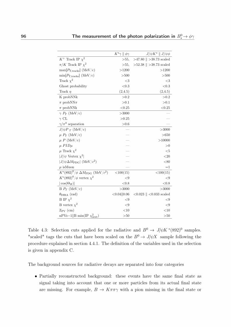
96 The measurement of the photon polarization in B0s → φγ
K γ ‖ φγ J/ψK ‖ J/ψφ
K+ Track IP χ2 >55, >47.80 ‖ >38.73 scaledπ/K Track IP χ2 >55, >52.38 ‖ >38.73 scaledmax[PT,tracks] (MeV/c) >1200 >1200min[PT,tracks] (MeV/c) >500 >500Track χ2 <3 <3Ghost probability <0.3 <0.3Track η (2,4.5) (2,4.5)K probNNk >0.2 >0.2π probNNπ >0.1 >0.1π probNNk <0.25 <0.25γ PT (MeV/c) >3000 —γ CL >0.25 —γ/π0 separation >0.6 —J/ψP T (MeV/c) — >3000μ PT (MeV/c) — >650μ P (MeV/c) — >10000μ PIDμ — >0μ Track χ2 — <5|J/ψ Vertex χ2| — <20|J/ψΔMPDG| (MeV/c2) — <80μ isMuon — =1K∗(892)0/φ ΔMPDG (MeV/c2) <100(15) <100(15)K∗(892)0/φ vertex χ2 <9 <9| cos(ΘH)| <0.8 <0.8B PT (MeV/c) >3000 >3000θDIRA (rad) <0.04‖0.06 <0.023 ‖ <0.033 scaledB IP χ2 <9 <9B vertex χ2 <9 <9ZPV (cm) <10 <10nPVs=1‖B min(IP χ2
next) >50 >50
Table 4.3: Selection cuts applied for the radiative and B0 → J/ψK ∗(892)0 samples."scaled" tags the cuts that have been scaled on the B0 → J/ψX sample following theprocedure explained in section 4.4.1. The definition of the variables used in the selectionis given in appendix C.
The background sources for radiative decays are separated into four categories
• Partially reconstructed background: these events have the same final state assignal taking into account that one or more particles from its actual final stateare missing. For example, B → Kππγ with a pion missing in the final state or
4.2 Signal and control channels selection 97
B → Kπππ0 with a pion missing in the final state and the π0 is misidentified as aphoton as background for B0→ K∗(892)0γ.
• Decays with π0 in the final state as B0 → Kππ0 background in B0→ K∗(892)0γ
where the π0 can be misidentified as a photon. Such decays constitute almost 50%of the peaking backgrounds and are reduced by the γ/π0separation cut and thehelicity angle cut.
• The baryonic radiative decay, Λb → Λ∗γ, is one of the peaking backgrounds underthe signal distribution.
• Background of the type B → Xγ in the B0→ K∗(892)0γ where X can be a φ, ρ orw (mis-ID reflections). This background is present when a misidentification in oneof the final state particles occurs. For example B0
s → φγ can contribute when oneof the kaons from the φ decays is misidentified as a pion. B0 → ρ0γ contributeswhen one of the pions from the ρ0 decays is misidentified as a kaon.
It is important to mention that in the case of B0s → φγ, the background is much reduced
thanks to the narrow φ resonance.
The background subtraction method used in this analysis is the sPlot technique [95].The sPlot technique is a statistical tool that unfolds the contributions of the differentsources to the distribution of a data sample in a given variable “v”. It can, on a sta-tistical basis, subtract the background contributions from the data sample by assigningweights accordingly to the different contributions modeled in the sample. The validityof this technique is based on two main criteria. The first one is that the variable “v”has a good discriminating power between the different contributions to the distribution.The second criterium is that this variable “v” must be uncorrelated with other variablesespecially the ones that is used for the analysis, in this case the proper time. The bestchoice of such a variable is the invariant mass.In the invariant mass distribution, the different contributions of signal and backgroundare modeled to a very good approximation. Moreover, the proper time evaluated witha B mass constraint, as explained in section 4.3.2.1, is uncorrelated with the invariantmass.Therefore, to subtract the background, the invariant mass distribution is fitted takinginto account the different background contributions and then the sPlot technique is ap-plied. The use of sPlot guaranties, to a very good extent, that the signal events are
98 The measurement of the photon polarization in B0s → φγ
separated from the background one on a statistical basis.
As for the di-muon channels, the background sources are mainly:
• Combinatorial background.
• Partially reconstructed backgrounds as B0→ J/ψK ∗(892)0 + pion background forB0→ J/ψK ∗(892)0 signal.
• The mis-ID reflection in B0→ J/ψK ∗(892)0 (B0s → J/ψφ) from B0
s → J/ψφ (B0→J/ψK ∗(892)0).
• Background from Λb → (pK)J/ψ assuming a proton misidentification.
The mass models for radiative and di-muon decays are explained in the following. Themass fits are performed as extended unbinned likelihood fits using RooFit [99].
A 0.5 % bias in the reconstructed B mass of radiative decays has been observed. Theorigin of this bias is due to a photon energy bias of the order of 1 % at high energy.This bias is due to the calorimeter calibration at low energies using π0 [54]. In radiativeanalysis [100], an ad-hoc calibration has been applied to the photon energy, the mass ishenceforth calibrated. Photon calibration is explained in appendix B.
4.2.3.1 Mass model for radiative channels
Once the expected background contaminations are determined, the mass fit is built.In the final mass fit to the B0 → K∗(892)0γ (B0
s → φγ) signal, the normalizationof all the background components is left free with the exception of Λb → Λ(pK)γ,B0 → K∗(892)0π0 (B0
s → φπ0) and B0s → φγ for B0 → K∗(892)0γ signal. The fit
function to the invariant mass of B0 (B0s ) is built as an extended PDF
P(m) = NS · S(m) +∑i
Ni · Bi(m) (4.7)
where S(m) is the signal PDF and Bi(m) is the background PDF where the index i
refers to the different contributions of the background. The invariant mass fit model isdefined as
4.2 Signal and control channels selection 99
• Combinatorial background is modeled with an exponential function.
Comb(m; τ) = exp(m/τ) (4.8)
• Partially reconstructed background
– Partially reconstructed background with a pion/kaon missing (B+ → K+π−π+γ
or B → φK+γ) is modeled with an Argus PDF [101] convoluted with a Gaus-sian resolution with the parameters fixed from simulation
Partial(m; c, p, μ,σ ) = Argus(m; c, μ− μ0, p)⊗ Gauss(0, σ) (4.9)
where μ0 = mπ for B0→ K∗(892)0γ and μ0 = mK for B0s → φγ.
– Partially reconstructed background of B0 → K+π−π0X for B0→ K∗(892)0γ
channel is modeled with an exponentially modified Gaussian (EMG) function,with parameters fixed from simulation except for the yields.
EMG(m;μ, σ,λ ) =λ
2e
λ2(2x+λσ2−2μ) · erfc(x+ λσ2 − μ√
2σ) (4.10)
• Background from Λ0b is modeled with a Crystal-Ball function [102], with parameters
fixed from simulation
• Background from B0 → Kππ0 is modeled with a Crystal-Ball function, with pa-rameters fixed from simulation. Since there is no simulated sample for B0
s → φπ0,the parameters are assumed to be the same as B0 → Kππ0 reconstructed asB0→ K∗(892)0γ, with mean value shifted due to higher B0
s mass.
• Background from B → V γ , with V being either ρ, φ or ω, is modeled with a PDFconsisting of two gaussian components.
4.2.3.2 Mass model for di-muon channels
The fit model for B0→ J/ψK ∗(892)0 mass spectrum has the following components
• Combinatorial background modeled by an exponential function:
Comb(m; τ) = exp (m/τ)
100 The measurement of the photon polarization in B0s → φγ
• Partially reconstructed B0 → J/ψK ∗(892)0 + pion modeled by an Argus [101]convoluted with a Gaussian resolution:
Partial(m; c, p, μ,σ ) = Argus(m; c, μ− μ0, p) ∗ Gauss(0, σ)
• The mis-ID reflection from B0 → J/ψφ, i.e. reconstructing B0 → J/ψφ as beingB0→ J/ψK ∗(892)0 by misidentifying one of the kaons to be a pion, modeled by adouble tail Crystal-Ball function [102] with parameters fixed from MC simulation:
CB(m;μ, σ, α, n) =
⎧⎪⎪⎪⎪⎪⎨⎪⎪⎪⎪⎪⎩AL(BL − m− μ
σ)−nL , for
m− μ
σ≤ −αL
exp(−(m− μ)2
2σ2), for − αL <
m− μ
σ< αR
AR(BR +m− μ
σ)−nR , for
m− μ
σ≥ αR
where αL(R) > 0 and
Ai = (ni
|αi|)ni exp(−|αi|2
2)
Bi =ni
|αi| − |αi|
• The background from Λb → (pK)J/ψ modeled by an Argus convoluted with aGaussian resolution:
Partial(m; c, p, μ,σ ) = Argus(m; c, μ− μ0, p) ∗ Gauss(0, σ)
• The signal B0 → J/ψK ∗(892)0 is modeled by a CB function with an Apollonioscore [103] and tail parameters fixed from MC simulation:
A(m;μ, b, δ, a, n) ∝⎧⎨⎩e−b
√1+ t2
b , if t ≥ −a
e−b.A × (1− anA
.(a+ t))−n , otherwise
where t is the reduced mass t = (m−μ)δ
and A =√
1 + a2
b.
A similar model is used for the B0s → J/ψφ mass fit.
The yields for the mis-ID reflections are constrained to the signal yield using gaussianconstraints calculated from the ratios of branching fractions and of selection efficiencies,
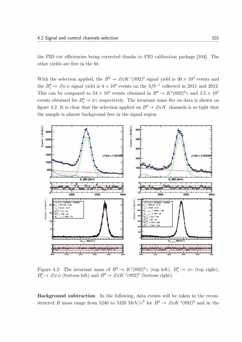
4.2 Signal and control channels selection 101
the PID cut efficiencies being corrected thanks to PID calibration package [104]. Theother yields are free in the fit.
With the selection applied, the B0 → J/ψK ∗(892)0 signal yield is 30 × 103 events andthe B0
s → J/ψφ signal yield is 4 × 10³ events on the 3fb−1 collected in 2011 and 2012.This can be compared to 24 × 103 events obtained in B0 → K∗(892)0γ and 3.5 × 10³
events obtained for B0s → φγ respectively. The invariant mass fits on data is shown on
figure 4.2. It is clear that the selection applied on B0→ J/ψX channels is so tight thatthe sample is almost background free in the signal region.
���� �2)�ψ�=)φ<
���������������� �!�
�
��
���
���
�����&�����±��>�%�&�������ψ�=)φ�γ
��&�6±�>���45�&�6��*
µ
��&45±�>����&�4��*
σ
�4�±�>�������<;&ψ�=)φ�
���±�>��������$�&ψ�=)φ�
�5�±�>�������ψ�=)φ�→��*�
���� ���� ���� �4�� ���� ����%�
�
�
���� �2)��ψ�=)?�@<
���������������� �!�
�
���
���
���
���
����
����
����
��&�����±��>�%�&�������Aψ=)?��@γ��&��±�>�����4&64�
'*µ
��&��±�>����&���'*
σ
����±�>��4�4�5�ψ=)?��@→�'*
����±�>��4���ψ=)?��@→��*
�
����±�>���44��$�&Λ
ψ=)?�@��4�±�>���6�
�$�&�*
ψ=)?�@��4�6±�>���4�����<;&
ψ=)?�@����4±�>���645���$�&
ψ=)?�@�
���� ���� ���� �4�� ���� ����%�
�
�
Figure 4.2: The invariant mass of B0 → K∗(892)0γ (top left), B0s → φγ (top right),
B0s → J/ψφ (bottom left) and B0→ J/ψK ∗(892)0 (bottom right).
Background subtraction In the following, data events will be taken in the recon-structed B mass range from 5240 to 5320 MeV/c2 for B0 → J/ψK ∗(892)0 and in the
102 The measurement of the photon polarization in B0s → φγ
range 5326 and 5406 for B0s → J/ψφ. As shown in figure 4.2, backgrounds are negligible
in this region and hence, no dedicated background subtraction is needed.
As for the radiative channels, the sPlot technique [95] is used. Peaking backgrounds aretaken as part of the signal distribution when performing the sPlot since for this type ofbackground, the yields are fixed.
An alternative background subtraction method is also used by our collaborators. Thismethod consists in evaluating the proper time distribution of the different backgroundsfrom simulation and subtract it from the proper time distribution in data using theyields obtained for each type of background from the mass fit. For the combinatorialbackground, the proper time distribution in the sidebands of the mass distribution of thedata is subtracted from the whole proper time distribution. This background subtractionmethod is indifferent to the correlations between the mass and proper time in contraryto the sPlot technique.
4.3 The proper time
4.3.1 The proper time reconstruction
The proper time is reconstructed as
ct =L
βγ=
M
P× L (4.11)
where L is the measured flight distance between the PV and the SV, M and P arethe measured mass and momentum of the B meson. The proper time results from anadjustment with a B mass constraint applied. The choice of the B mass constrainedproper time improves the proper time resolution. Moreover, this proper time has, bydefinition, uncorrelated errors with the reconstructed B mass. This is essential for theuse of the sPlot technique [95] since this technique requires that the variable used tounfold the different contributions in the data sample should be uncorrelated with theother variables that are used to perform the analysis.
The photon energy bias (appendix B) affects the proper time. This effect has beenstudied and corrected for, the procedure is explained in section 4.3.2.3.
4.3 The proper time 103
4.3.2 Proper time distribution model for signal
The probability density function used to fit the proper time is defined as
PDF = [Decay rate× Acceptance] ∗ Resolution
where decay rate =
⎧⎨⎩e−t/τB0 for B0→ K∗(892)0γ and B0→ J/ψK∗(892)0
e−t/τ
B0s × (cosh(ΔΓst/2)− AΔ × sinh(ΔΓst/2) for B0
s → φγ,
acceptance =(a[t− t0])
n
1 + (a[t− t0])n× e−δΓt
and resolution = e−b
√√√√1+
(t− μ)2
σ2 . (4.12)
The time-dependent decay rate is introduced in 4.1. It can be seen that for the B sys-tem, the decay rate reduces down to a single exponential when neglecting ΔΓ. Whereasfor the B0
s system the decay rate maintains the form with the hyperbolic sine and cosine.
The proper time resolution model is discussed in section 4.3.2.1. In the same section,proper time bias and its correction are discussed. The proper time acceptance and itsparameterization are discussed in section 4.3.2.4.
An unbinned maximum likelihood fit is applied to the proper time distribution of theselected events using the Likelihood defined in 4.12 to extract AΔ.
4.3.2.1 Proper time resolution
The proper time resolution obtained for the radiative decays is of the order of 40-50 fs.This resolution is evaluated using simulation. The effect of non perfect knowledge ofthe proper time resolution on the measurement of AΔ has been studied in [105] and hasbeen found to be negligible. Nevertheless, understanding and modeling the proper timeresolution is an important issue.
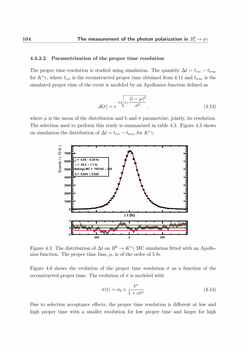
104 The measurement of the photon polarization in B0s → φγ
4.3.2.2 Parametrization of the proper time resolution
The proper time resolution is studied using simulation. The quantity Δt = trec − ttrue
for K∗γ, where trec is the reconstructed proper time obtained from 4.11 and ttrue is thesimulated proper time of the event is modeled by an Apollonios function defined as
A(t) = e−b
√√√√1+
(t− μ)2
σ2 . (4.13)
where μ is the mean of the distribution and b and σ parametrize, jointly, its resolution.The selection used to perform this study is summarized in table 4.3. Figure 4.3 showson simulation the distribution of Δt = trec − ttrue for K∗γ.
������Δ
�����������"#�����
�
����
����
4���
����
����
����
5���
��&����±�>���&���µ
��&���±�>��46&��σ
�4��±��+����� :�>���������
��&�4�±;�>���&����
%��� � ���%�
�
�
Figure 4.3: The distribution of Δt on B0 → K∗γ MC simulation fitted with an Apollo-nios function. The proper time bias, μ, is of the order of 5 fs.
Figure 4.6 shows the evolution of the proper time resolution σ as a function of thereconstructed proper time. The evolution of σ is modeled with
σ(t) = σ0 × tn
1 + αtn(4.14)
Due to selection acceptance effects, the proper time resolution is different at low andhigh proper time with a smaller resolution for low proper time and larger for high
4.3 The proper time 105
proper time. This is shown in figures 4.4 and 4.5 for B0→ K∗(892)0γ events where theΔt distribution is fitted in different bins of the proper time with an Apollonios functionfixing the parameter b to the fit value over the whole proper time range so as to evolutionof σ. The resolution increases starting from 26 fs for a proper time in [0,0.5] ps rangeand going up to 59 fs for a proper time in [6.5,10] ps range.
Resolution parameters K∗γ J/ψK∗ φγ J/ψφ
μ fs 4.04 ± 0.20 1.61 ± 0.34 4.38 ± 0.29 2.62 ± 0.17b 1.11 ± 0.06 0.87 ± 0.06 1.11 ± 0.06 0.89 ± 0.03σ0 fs 110.4 ± 10.0 143.7 ± 12.1 115.3 ± 9.9 174.1 ± 8.2α 1.78 ± 0.24 2.51 ± 0.32 1.73 ± 0.22 2.90 ± 0.17n 0.62 ± 0.06 0.84 ± 0.08 0.65 ± 0.05 0.82 ± 0.03
Table 4.4: Resolution parameters of the radiative and di-muon channels obtained fromMC.
In the proper time fits, the proper time resolution parameter of equation (4.13) isparametrized according to this. Table 4.4 summarizes the resolution parameters ob-tained from MC for the radiative and di-muon channels.
4.3.2.3 Proper time bias study
The procedure to correct the photon energy-induced bias in the proper time is discussedin this section.
To investigate the bias properly, the distribution of Δt = trec − ttrue for K∗γ is plottedfor each photon type (converted or unconverted) and for each region of the calorimeter(inner, middle or outer). The distribution is fitted with an Apollonios function. Figures4.7 show the fits to B0
s → φγ MC events of unconverted photon type (as per example,same conclusion is obtained for converted photons). Table 4.5 summarizes the results ofthe fits for the different categories of the fits (converted or unconverted: inner, middleand outer calorimeter regions).
It can be easily seen, looking at the means of the Apollonios function reported in table4.5, that the distribution Δt is biased: ∼6 fs, ∼15 fs and ∼30 fs for the outer, middleand inner regions of the calorimeter respectively.
Calibrating the momentum of the B by calibrating the photon momentum (appendixB), reduced the proper time bias to a residual bias of about 5 fs constant over the dif-ferent calorimeter regions and the different photon types. The calibration is performed
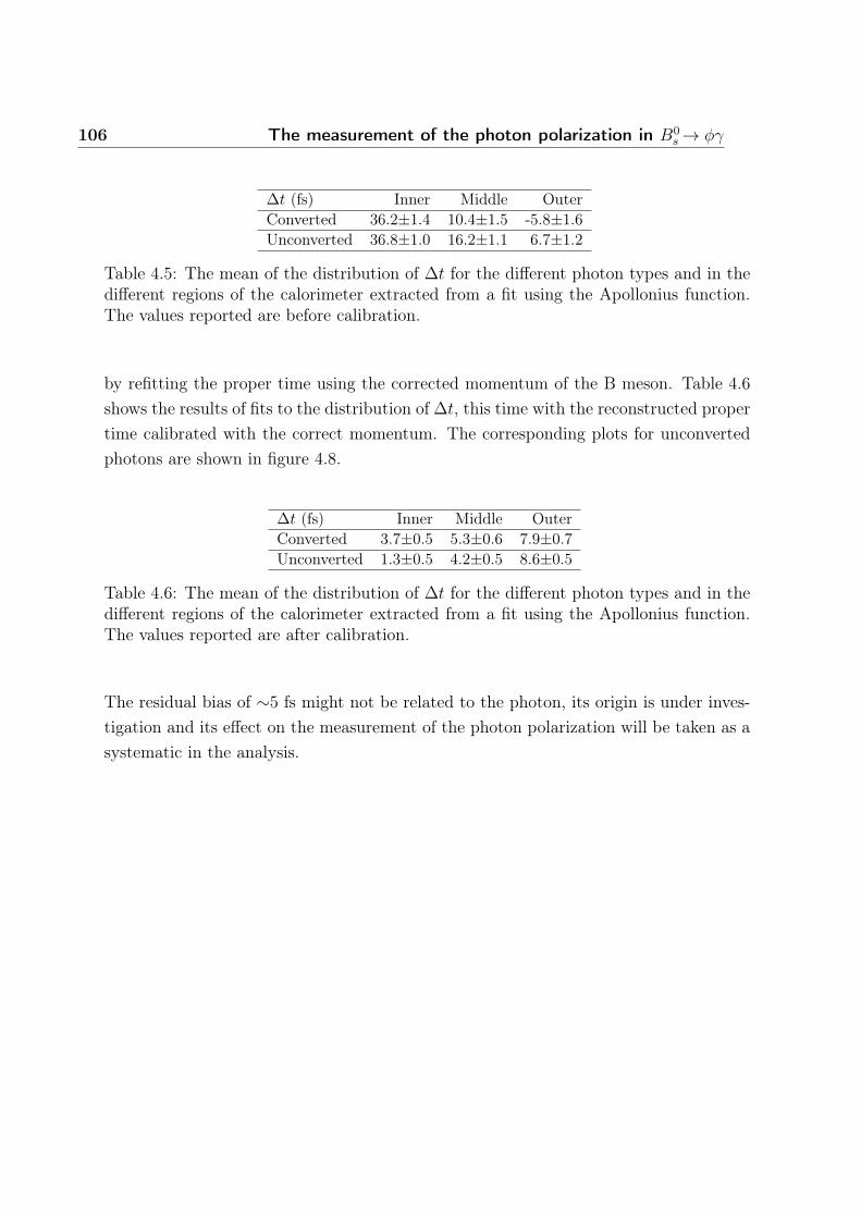
106 The measurement of the photon polarization in B0s → φγ
Δt (fs) Inner Middle OuterConverted 36.2±1.4 10.4±1.5 -5.8±1.6Unconverted 36.8±1.0 16.2±1.1 6.7±1.2
Table 4.5: The mean of the distribution of Δt for the different photon types and in thedifferent regions of the calorimeter extracted from a fit using the Apollonius function.The values reported are before calibration.
by refitting the proper time using the corrected momentum of the B meson. Table 4.6shows the results of fits to the distribution of Δt, this time with the reconstructed propertime calibrated with the correct momentum. The corresponding plots for unconvertedphotons are shown in figure 4.8.
Δt (fs) Inner Middle OuterConverted 3.7±0.5 5.3±0.6 7.9±0.7Unconverted 1.3±0.5 4.2±0.5 8.6±0.5
Table 4.6: The mean of the distribution of Δt for the different photon types and in thedifferent regions of the calorimeter extracted from a fit using the Apollonius function.The values reported are after calibration.
The residual bias of ∼5 fs might not be related to the photon, its origin is under inves-tigation and its effect on the measurement of the photon polarization will be taken as asystematic in the analysis.
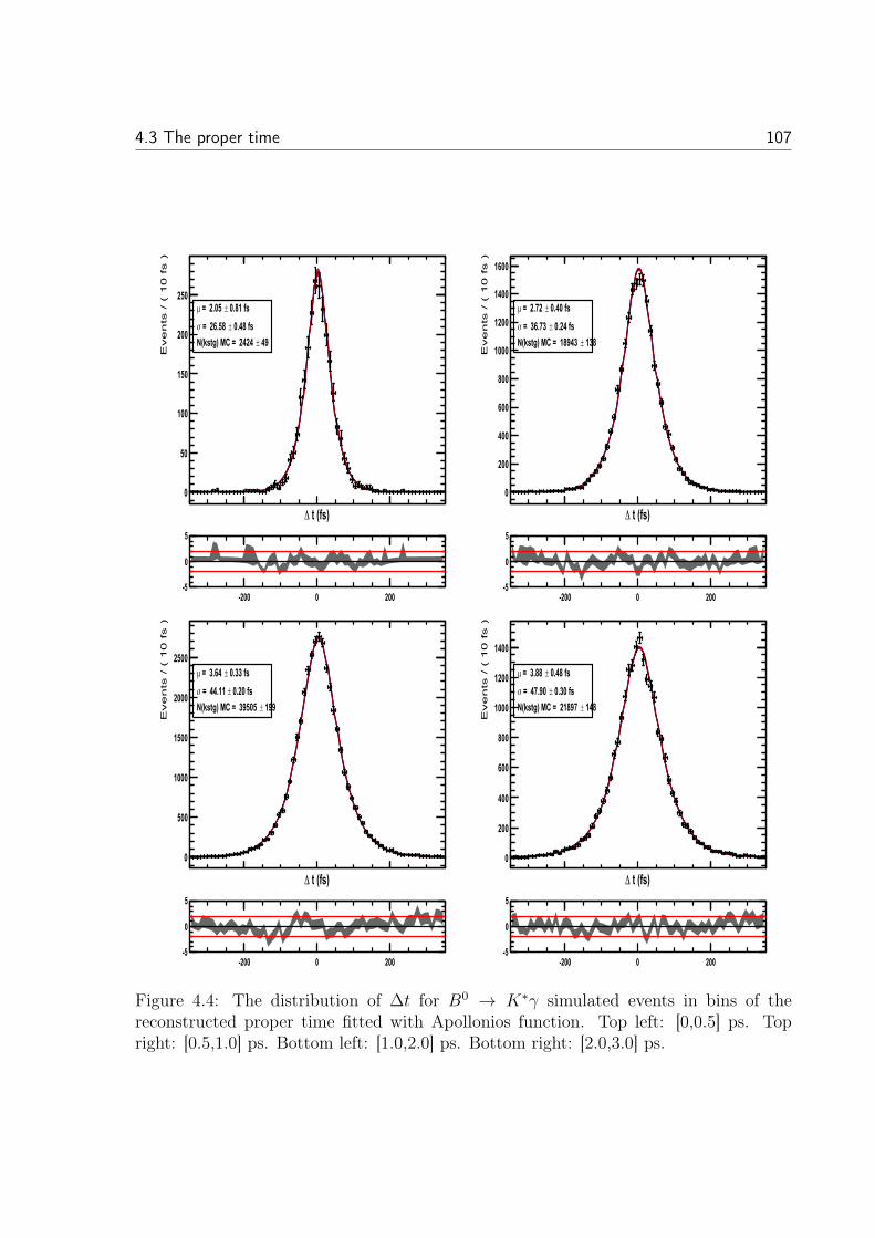
4.3 The proper time 107
������Δ
�����������"#�����
�
��
���
���
���
�����&����±�>���&���µ
��&����±�>����&���σ
��6±��+����� :�>�������
%��� � ���%�
�
�
������Δ
�����������"#�����
�
���
���
���
���
����
����
����
����
��&����±�>���&5��µ
��&����±�>��4�&54�σ
��4�±��+����� :�>����6�4�
%��� � ���%�
�
�
������Δ
�����������"#�����
�
���
����
����
����
������&44��±�>��4&���µ
��&����±�>����&���σ
��66±��+����� :�>��46����
%��� � ���%�
�
�
������Δ
�����������"#�����
�
���
���
���
���
����
����
����
��&����±�>��4&���µ
��&4���±�>���5&6��σ
����±��+����� :�>�����65�
%��� � ���%�
�
�
Figure 4.4: The distribution of Δt for B0 → K∗γ simulated events in bins of thereconstructed proper time fitted with Apollonios function. Top left: [0,0.5] ps. Topright: [0.5,1.0] ps. Bottom left: [1.0,2.0] ps. Bottom right: [2.0,3.0] ps.
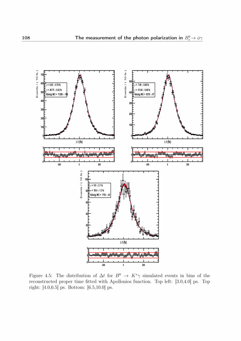
108 The measurement of the photon polarization in B0s → φγ
������Δ
�����������"#�����
�
���
���
4��
���
���
���
5��
��&5���±�>���&���µ
��&�4��±�>���6&5��σ
����±��+����� :�>������6�
%��� � ���%�
�
�
������Δ
�����������"#�����
�
���
���
4��
���
�����&����±�>��5&�6�µ
��&�6��±�>����&���σ
�65±��+����� :�>��645��
%��� � ���%�
�
�
������Δ
�����������"#�����
�
��
��
��
��
���
��&���±�>��6&6�µ
��&4��±�>���6&��σ
���±��+����� :�>���5�4�
%��� � ���%�
�
�
Figure 4.5: The distribution of Δt for B0 → K∗γ simulated events in bins of thereconstructed proper time fitted with Apollonios function. Top left: [3.0,4.0] ps. Topright: [4.0,6.5] ps. Bottom: [6.5,10.0] ps.
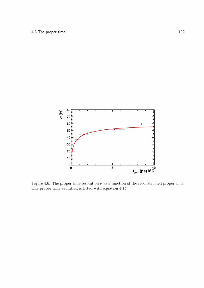
4.3 The proper time 109
������ :γ@?�� � ��
�����
σ
�
��
��
4�
��
��
��
5�
��
Figure 4.6: The proper time resolution σ as a function of the reconstructed proper time.The proper time evolution is fitted with equation 4.14.
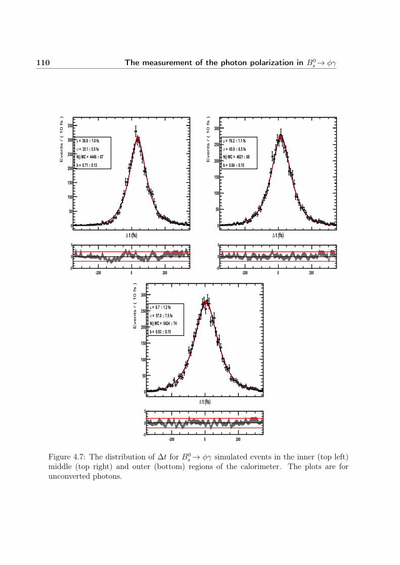
110 The measurement of the photon polarization in B0s → φγ
������Δ
�����������"#�����
�
��
���
���
���
���
4��
4��
��&���±�>��4�&��µ
��&���±�>��4�&��σ
��5±���� :�>���������&�4±;�>���&5��
%��� � ���%�
�
�
������Δ
�����������"#�����
�
��
���
���
���
���
4��
��&���±�>����&��µ
��&���±�>����&6�σ
���±���� :�>���������&��±;�>���&���
%��� � ���%�
�
�
������Δ
�����������"#�����
�
��
���
���
���
���
4��
��&���±�>���&5�µ
�5&���±�>���5&��σ
�5�±���� :�>���������&��±;�>���&64�
%��� � ���%�
�
�
Figure 4.7: The distribution of Δt for B0s → φγ simulated events in the inner (top left)
middle (top right) and outer (bottom) regions of the calorimeter. The plots are forunconverted photons.
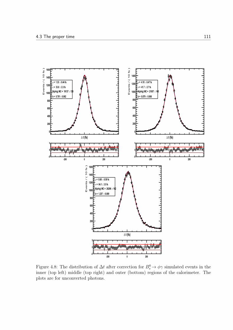
4.3 The proper time 111
������Δ
�����������"#�����
�
���
���
���
���
����
����
����
����
��&����±�>���&44�µ
��&4��±�>��44&��σ
��4�±�������� :�>���6�45�
��&���±;�>���&5���
%��� � ���%�
�
�
������Δ
�����������"#�����
�
���
���
���
���
����
����
����
��&�5��±�>���&���µ
��&5��±�>����&5�σ
����±�������� :�>������5�
��&���±;�>���&�56�
%��� � ���%�
�
�
������Δ
�����������"#�����
�
���
���
���
���
����
����
����
����
��&����±�>���&���µ
�4&���±�>����&��σ
����±�������� :�>�����6��
��&��6±;�>���&��5�
%��� � ���%�
�
�
Figure 4.8: The distribution of Δt after correction for B0s → φγ simulated events in the
inner (top left) middle (top right) and outer (bottom) regions of the calorimeter. Theplots are for unconverted photons.
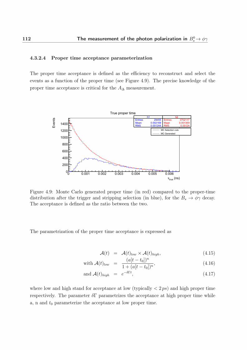
112 The measurement of the photon polarization in B0s → φγ
4.3.2.4 Proper time acceptance parameterization
The proper time acceptance is defined as the efficiency to reconstruct and select theevents as a function of the proper time (see Figure 4.9). The precise knowledge of theproper time acceptance is critical for the AΔ measurement.
$���� ���� �%&#�""& ����� �#'##"%()* +��� �#'##"��
������ ��τ# #'##" #'##� #'##% #'##� #'##, #'##(
������
#
�##
�##
(##
-##
"###
"�##
"�##
$���� ���� �%&#�""& ����� �#'##"%()* +��� �#'##"��
$"��� ���� ��)�,, ����� �#'##�"()* +��� �#'##"���
. ���/ �/� ���0�
��+�1��������� ������ �����
Figure 4.9: Monte Carlo generated proper time (in red) compared to the proper-timedistribution after the trigger and stripping selection (in blue), for the Bs → φγ decay.The acceptance is defined as the ratio between the two.
The parametrization of the proper time acceptance is expressed as
A(t) = A(t)low ×A(t)high, (4.15)
with A(t)low =(a[t− t0])
n
1 + (a[t− t0])n, (4.16)
and A(t)high = e−δΓt, (4.17)
where low and high stand for acceptance at low (typically < 2 ps) and high proper timerespectively. The parameter δΓ parametrizes the acceptance at high proper time whilea, n and t0 parameterize the acceptance at low proper time.
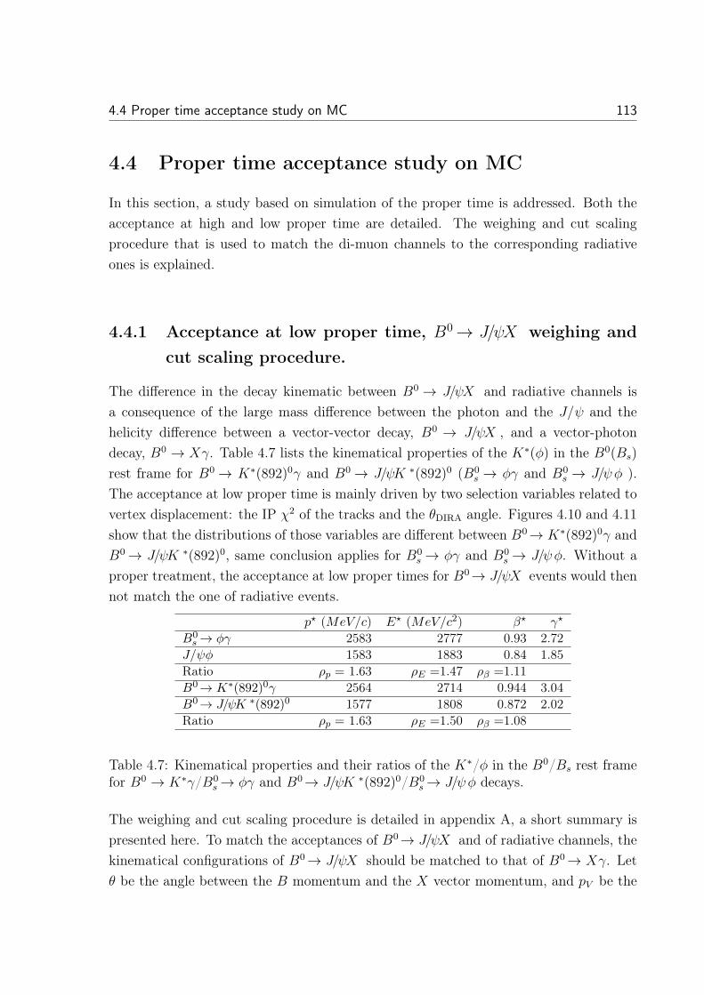
4.4 Proper time acceptance study on MC 113
4.4 Proper time acceptance study on MC
In this section, a study based on simulation of the proper time is addressed. Both theacceptance at high and low proper time are detailed. The weighing and cut scalingprocedure that is used to match the di-muon channels to the corresponding radiativeones is explained.
4.4.1 Acceptance at low proper time, B0→ J/ψX weighing andcut scaling procedure.
The difference in the decay kinematic between B0 → J/ψX and radiative channels isa consequence of the large mass difference between the photon and the J/ψ and thehelicity difference between a vector-vector decay, B0 → J/ψX , and a vector-photondecay, B0 → Xγ. Table 4.7 lists the kinematical properties of the K∗(φ) in the B0(Bs)
rest frame for B0 → K∗(892)0γ and B0 → J/ψK ∗(892)0 (B0s → φγ and B0
s → J/ψφ ).The acceptance at low proper time is mainly driven by two selection variables related tovertex displacement: the IP χ2 of the tracks and the θDIRA angle. Figures 4.10 and 4.11show that the distributions of those variables are different between B0→ K∗(892)0γ andB0 → J/ψK ∗(892)0, same conclusion applies for B0
s → φγ and B0s → J/ψφ. Without a
proper treatment, the acceptance at low proper times for B0→ J/ψX events would thennot match the one of radiative events.
p (MeV/c) E (MeV/c2) β γ
B0s → φγ 2583 2777 0.93 2.72
J/ψφ 1583 1883 0.84 1.85Ratio ρp = 1.63 ρE =1.47 ρβ =1.11B0→ K∗(892)0γ 2564 2714 0.944 3.04B0→ J/ψK ∗(892)0 1577 1808 0.872 2.02Ratio ρp = 1.63 ρE =1.50 ρβ =1.08
Table 4.7: Kinematical properties and their ratios of the K∗/φ in the B0/Bs rest framefor B0 → K∗γ/B0
s → φγ and B0→ J/ψK ∗(892)0/B0s → J/ψφ decays.
The weighing and cut scaling procedure is detailed in appendix A, a short summary ispresented here. To match the acceptances of B0→ J/ψX and of radiative channels, thekinematical configurations of B0→ J/ψX should be matched to that of B0→ Xγ. Letθ be the angle between the B momentum and the X vector momentum, and pV be the
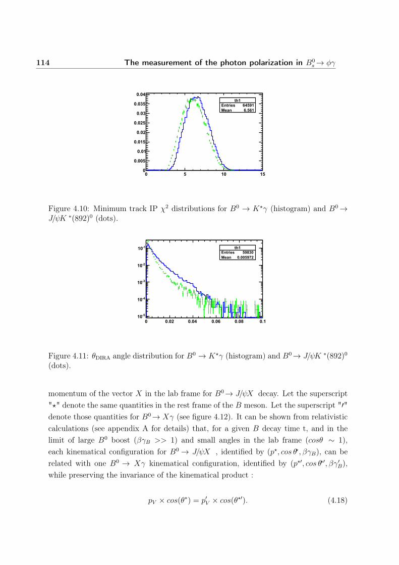
114 The measurement of the photon polarization in B0s → φγ
� � �� ���
�&���
�&��
�&���
�&��
�&���
�&�4
�&�4�
�&�����
��$���� ����6� ����� ���&���
Figure 4.10: Minimum track IP χ2 distributions for B0 → K γ (histogram) and B0→J/ψK ∗(892)0 (dots).
� �&�� �&�� �&�� �&�� �&�%���
%���
%4��
%���
%��� �����$���� ��6�4� ����� ��&���65�
Figure 4.11: θDIRA angle distribution for B0 → K γ (histogram) and B0→ J/ψK ∗(892)0
(dots).
momentum of the vector X in the lab frame for B0→ J/ψX decay. Let the superscript"�" denote the same quantities in the rest frame of the B meson. Let the superscript "′"denote those quantities for B0→ Xγ (see figure 4.12). It can be shown from relativisticcalculations (see appendix A for details) that, for a given B decay time t, and in thelimit of large B0 boost (βγB >> 1) and small angles in the lab frame (cosθ ∼ 1),each kinematical configuration for B0 → J/ψX , identified by (p , cos θ , βγB), can berelated with one B0 → Xγ kinematical configuration, identified by (p ′, cos θ ′, βγ′
B),while preserving the invariance of the kinematical product :
pV × cos(θ∗) = p′V × cos(θ ′). (4.18)
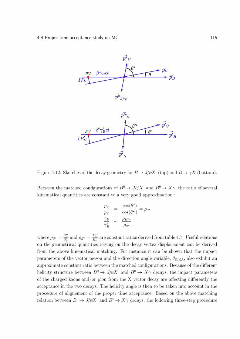
4.4 Proper time acceptance study on MC 115
Figure 4.12: Sketches of the decay geometry for B→ J/ψX (top) and B→ γX (bottom).
Between the matched configurations of B0→ J/ψX and B0→ Xγ, the ratio of severalkinematical quantities are constant to a very good approximation :
p′VpV
=cos(θ∗)cos(θ ′)
= ρβ∗
γBγ′B
∼ ρE∗∗ρβ∗
where ρβ� =β�′V
β�V
and ρE� =E�′
V
E�V
are constant ratios derived from table 4.7. Useful relationson the geometrical quantities relying on the decay vertex displacement can be derivedfrom the above kinematical matching. For instance it can be shown that the impactparameters of the vector meson and the direction angle variable, θDIRA, also exhibit anapproximate constant ratio between the matched configurations. Because of the differenthelicity structure between B0 → J/ψX and B0 → Xγ decays, the impact parametersof the charged kaons and/or pion from the X vector decay are affecting differently theacceptance in the two decays. The helicity angle is then to be taken into account in theprocedure of alignement of the proper time acceptance. Based on the above matchingrelation between B0→ J/ψX and B0→ Xγ decays, the following three-step procedure
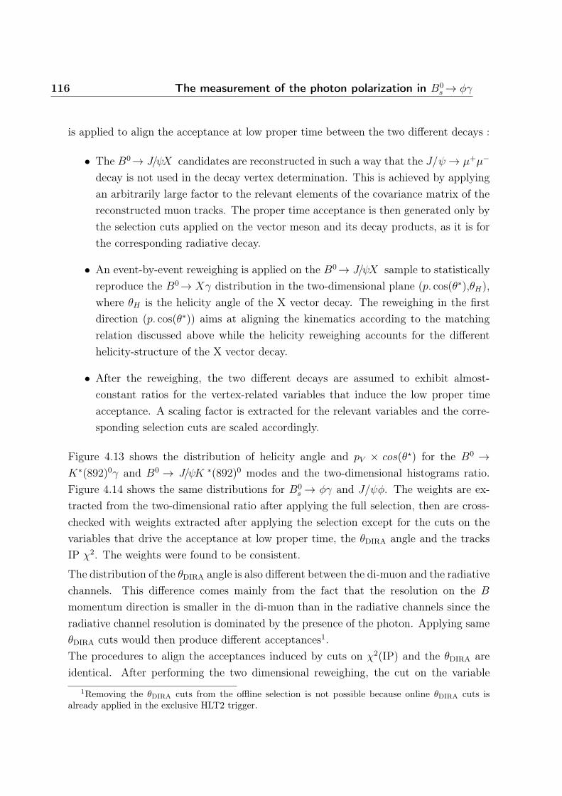
116 The measurement of the photon polarization in B0s → φγ
is applied to align the acceptance at low proper time between the two different decays :
• The B0→ J/ψX candidates are reconstructed in such a way that the J/ψ → μ+μ−
decay is not used in the decay vertex determination. This is achieved by applyingan arbitrarily large factor to the relevant elements of the covariance matrix of thereconstructed muon tracks. The proper time acceptance is then generated only bythe selection cuts applied on the vector meson and its decay products, as it is forthe corresponding radiative decay.
• An event-by-event reweighing is applied on the B0→ J/ψX sample to statisticallyreproduce the B0→ Xγ distribution in the two-dimensional plane (p. cos(θ∗),θH),where θH is the helicity angle of the X vector decay. The reweighing in the firstdirection (p. cos(θ∗)) aims at aligning the kinematics according to the matchingrelation discussed above while the helicity reweighing accounts for the differenthelicity-structure of the X vector decay.
• After the reweighing, the two different decays are assumed to exhibit almost-constant ratios for the vertex-related variables that induce the low proper timeacceptance. A scaling factor is extracted for the relevant variables and the corre-sponding selection cuts are scaled accordingly.
Figure 4.13 shows the distribution of helicity angle and pV × cos(θ ) for the B0 →K∗(892)0γ and B0 → J/ψK ∗(892)0 modes and the two-dimensional histograms ratio.Figure 4.14 shows the same distributions for B0
s → φγ and J/ψφ. The weights are ex-tracted from the two-dimensional ratio after applying the full selection, then are cross-checked with weights extracted after applying the selection except for the cuts on thevariables that drive the acceptance at low proper time, the θDIRA angle and the tracksIP χ2. The weights were found to be consistent.
The distribution of the θDIRA angle is also different between the di-muon and the radiativechannels. This difference comes mainly from the fact that the resolution on the B
momentum direction is smaller in the di-muon than in the radiative channels since theradiative channel resolution is dominated by the presence of the photon. Applying sameθDIRA cuts would then produce different acceptances1.The procedures to align the acceptances induced by cuts on χ2(IP) and the θDIRA areidentical. After performing the two dimensional reweighing, the cut on the variable
1Removing the θDIRA cuts from the offline selection is not possible because online θDIRA cuts isalready applied in the exclusive HLT2 trigger.
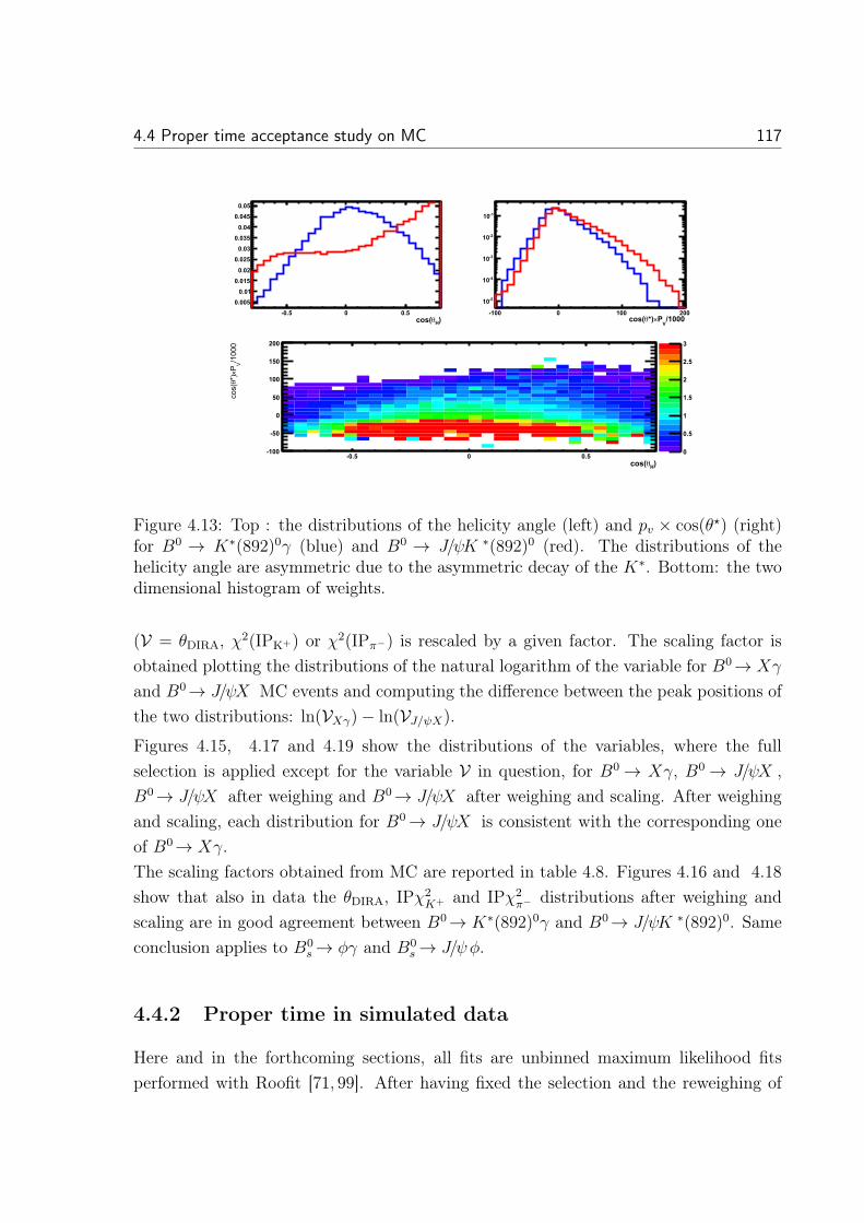
4.4 Proper time acceptance study on MC 117
�9���%�&� � �&�
�&����&���&����&��
�&����&�4�&�4��&��
�&����&��
)����2!×?�θ����
%��� � ��� ���
%���
%���
%4��
%���
%���
�9���%�&� � �&�
�"###
!2×3�θ
���
%���
%��
�
��
���
���
���
�
�&�
�
�&�
�
�&�
4
Figure 4.13: Top : the distributions of the helicity angle (left) and pv × cos(θ ) (right)for B0 → K∗(892)0γ (blue) and B0 → J/ψK ∗(892)0 (red). The distributions of thehelicity angle are asymmetric due to the asymmetric decay of the K∗. Bottom: the twodimensional histogram of weights.
(V = θDIRA, χ2(IPK+) or χ2(IPπ−) is rescaled by a given factor. The scaling factor isobtained plotting the distributions of the natural logarithm of the variable for B0→ Xγ
and B0→ J/ψX MC events and computing the difference between the peak positions ofthe two distributions: ln(VXγ)− ln(VJ/ψX).
Figures 4.15, 4.17 and 4.19 show the distributions of the variables, where the fullselection is applied except for the variable V in question, for B0 → Xγ, B0 → J/ψX ,B0→ J/ψX after weighing and B0→ J/ψX after weighing and scaling. After weighingand scaling, each distribution for B0→ J/ψX is consistent with the corresponding oneof B0→ Xγ.The scaling factors obtained from MC are reported in table 4.8. Figures 4.16 and 4.18show that also in data the θDIRA, IPχ2
K+ and IPχ2π− distributions after weighing and
scaling are in good agreement between B0→ K∗(892)0γ and B0→ J/ψK ∗(892)0. Sameconclusion applies to B0
s → φγ and B0s → J/ψφ.
4.4.2 Proper time in simulated data
Here and in the forthcoming sections, all fits are unbinned maximum likelihood fitsperformed with Roofit [71, 99]. After having fixed the selection and the reweighing of
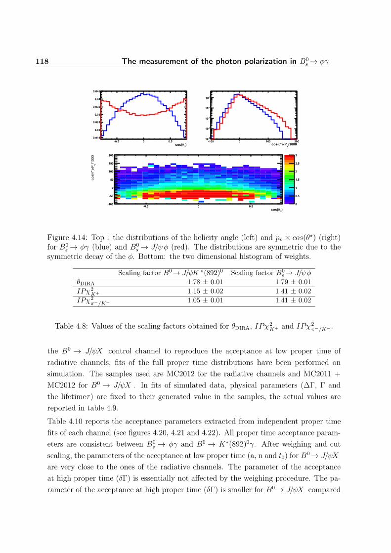
118 The measurement of the photon polarization in B0s → φγ
�9���%�&� � �&�
�&���
�&��
�&���
�&�4
�&�4�
�&��
�&���
)����2!×?�θ����
%��� � ��� ���%���
%���
%4��
%���
%���
�9���%�&� � �&�
�"###
!2×3�θ
���
%���
%��
�
��
���
���
���
�
�&�
�
�&�
�
�&�
4
Figure 4.14: Top : the distributions of the helicity angle (left) and pv × cos(θ ) (right)for B0
s → φγ (blue) and B0s → J/ψφ (red). The distributions are symmetric due to the
symmetric decay of the φ. Bottom: the two dimensional histogram of weights.
Scaling factor B0→ J/ψK ∗(892)0 Scaling factor B0s → J/ψφ
θDIRA 1.78 ± 0.01 1.79 ± 0.01IPχ2
K+ 1.15 ± 0.02 1.41 ± 0.02IPχ2
π−/K− 1.05 ± 0.01 1.41 ± 0.02
Table 4.8: Values of the scaling factors obtained for θDIRA, IPχ2K+ and IPχ2
π−/K− .
the B0 → J/ψX control channel to reproduce the acceptance at low proper time ofradiative channels, fits of the full proper time distributions have been performed onsimulation. The samples used are MC2012 for the radiative channels and MC2011 +MC2012 for B0 → J/ψX . In fits of simulated data, physical parameters (ΔΓ, Γ andthe lifetimeτ) are fixed to their generated value in the samples, the actual values arereported in table 4.9.
Table 4.10 reports the acceptance parameters extracted from independent proper timefits of each channel (see figures 4.20, 4.21 and 4.22). All proper time acceptance param-eters are consistent between B0
s → φγ and B0 → K∗(892)0γ. After weighing and cutscaling, the parameters of the acceptance at low proper time (a, n and t0) for B0→ J/ψX
are very close to the ones of the radiative channels. The parameter of the acceptanceat high proper time (δΓ) is essentially not affected by the weighing procedure. The pa-rameter of the acceptance at high proper time (δΓ) is smaller for B0→ J/ψX compared
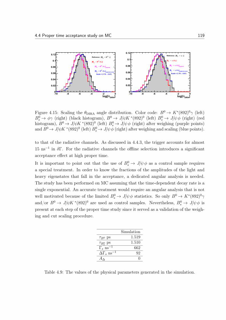
4.4 Proper time acceptance study on MC 119
B��C3���D%�� %� %� %� %� ��
�&��
�&��
�&��
�&��
�&�
�&��Bγ�?��@→�
'�C��$�����1�D*
Bψ�=)?��@→�'
�D*
/������'Bψ�=)?��@→�
'�D*
/������'E�����'Bψ�=)?��@→�
'�D*
��&���±�#�����>���&5��
B��C3���D%�� %� %� %� %� ��
�&��
�&��
�&��
�&��
�&�
�&��Bγ�φ�→���C��$�����1�D*
Bψ�=)φ�→���D*
/������'Bψ�=)φ�→���D*
/������'E�����'Bψ�=)φ�→���D*
��&���±�#�����>���&56�
Figure 4.15: Scaling the θDIRA angle distribution. Color code: B0 → K∗(892)0γ (left)B0
s → φγ (right) (black histogram), B0 → J/ψK ∗(892)0 (left) B0s → J/ψφ (right) (red
histogram), B0→ J/ψK ∗(892)0 (left) B0s → J/ψφ (right) after weighing (purple points)
and B0→ J/ψK ∗(892)0 (left) B0s → J/ψφ (right) after weighing and scaling (blue points).
to that of the radiative channels. As discussed in 4.4.3, the trigger accounts for almost15 ns−1 in δΓ. For the radiative channels the offline selection introduces a significantacceptance effect at high proper time.
It is important to point out that the use of B0s → J/ψφ as a control sample requires
a special treatment. In order to know the fractions of the amplitudes of the light andheavy eigenstates that fall in the acceptance, a dedicated angular analysis is needed.The study has been performed on MC assuming that the time-dependent decay rate is asingle exponential. An accurate treatment would require an angular analysis that is notwell motivated because of the limited B0
s → J/ψφ statistics. So only B0 → K∗(892)0γ
and/or B0 → J/ψK ∗(892)0 are used as control samples. Nevertheless, B0s → J/ψφ is
present at each step of the proper time study since it served as a validation of the weigh-ing and cut scaling procedure.
SimulationτB0 ps 1.519τB0
sps 1.510
Γs ns−1 662ΔΓs ns−1 92AΔ 0
Table 4.9: The values of the physical parameters generated in the simulation.
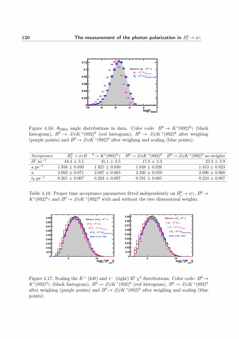
120 The measurement of the photon polarization in B0s → φγ
B��C3��D%�� %� %� %� %� ��
�&��
�&��
�&��
�&��
�&�
�&��
Bγ�?��@→�'
�C��$�����1�D*
/������'Bψ�=)?��@→�
'�D*
/������'E�����'Bψ�=)?��@→�
'�D*
Figure 4.16: θDIRA angle distributions in data. Color code: B0 → K∗(892)0γ (blackhistogram), B0 → J/ψK ∗(892)0 (red histogram), B0 → J/ψK ∗(892)0 after weighing(purple points) and B0→ J/ψK ∗(892)0 after weighing and scaling (blue points).
Acceptance B0s → φγB 0→ K∗(892)0γ B0→ J/ψK ∗(892)0 B0→ J/ψK ∗(892)0 no weights
δΓ ns−1 44.4 ± 3.5 45.1 ± 3.5 17.0 ± 3.3 23.3 ± 3.9a ps−1 1.956 ± 0.030 1.925 ± 0.030 1.838 ± 0.026 1.453 ± 0.023n 2.093 ± 0.071 2.087 ± 0.065 2.330 ± 0.059 2.096 ± 0.060t0 ps−1 0.201 ± 0.007 0.203 ± 0.007 0.191 ± 0.005 0.224 ± 0.007
Table 4.10: Proper time acceptance parameters fitted independently on B0s → φγ, B0→
K∗(892)0γ and B0→ J/ψK ∗(892)0 with and without the two dimensional weights.
�B<��
��!�χ���D� ��
�
�&���&���&�4�&��
�&���&���&�5�&��
�&�6Bγ�?��@→�
'0*E�C��$�����1�D@
Bψ�=)?��@→�'
0*E�D@
/������'Bψ�=)?��@→�
'0*E�D@
/������'E�����'Bψ�=)?��@→�
'0*E�D@
��&���±�#�����>���&���
�B<��
��!�χ���D� ��
�
�&��
�&��
�&�4
�&��
�&��
�&��
�&�5
�&��
�&�6Bγ�?��@→�
'0*%π�C��$�����1�D
Bψ�=)?��@→�'
0*%π�D
/������'Bψ�=)?��@→�
'0*%π�D
/������'E�����'Bψ�=)?��@→�
'0*%π�D
��&���±�#�����>���&���
Figure 4.17: Scaling the K+ (left) and π− (right) IP χ2 distributions. Color code: B0→K∗(892)0γ (black histogram), B0 → J/ψK ∗(892)0 (red histogram), B0 → J/ψK ∗(892)0
after weighing (purple points) and B0→ J/ψK ∗(892)0 after weighing and scaling (bluepoints).
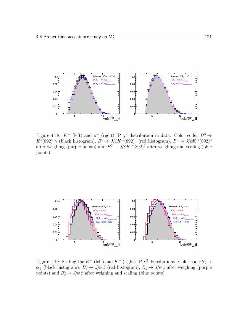
4.4 Proper time acceptance study on MC 121
�B<��
��!�χ���D� ��
�
�&��
�&��
�&��
�&��
�&� Bγ�?��@→�'
0*E�C��$�����1�D@
/������'Bψ�=)?��@→�
'0*E�D@
/������'E�����'Bψ�=)?��@→�
'0*E�D@
�B<��
��!�χ���D� ��
�
�&��
�&��
�&��
�&��
�&� Bγ�?��@→�'
0*%π�C��$�����1�D
/������'Bψ�=)?��@→�
'0*%π�D
/������'E�����'Bψ�=)?��@→�
'0*%π�D
Figure 4.18: K+ (left) and π− (right) IP χ2 distribution in data. Color code: B0 →K∗(892)0γ (black histogram), B0 → J/ψK ∗(892)0 (red histogram), B0 → J/ψK ∗(892)0
after weighing (purple points) and B0→ J/ψK ∗(892)0 after weighing and scaling (bluepoints).
�B<��
��!�χ���D� ��
�
�&��
�&��
�&��
�&��
�&�
Bγ�φ�→��0*E�C��$�����1�D@
Bψ�=)φ�→��0*E�D@
/������'Bψ�=)φ�→��0*
E�D@
/������'E�����'Bψ�=)φ�→��0*
E�D@
��&���±�#�����>���&���
�B<��
��!�χ���D� ��
�
�&��
�&��
�&��
�&��
�&�
Bγ�φ�→��0*%�C��$�����1�D@
Bψ�=)φ�→��0*%�D@
/������'Bψ�=)φ�→��0*
%�D@
/������'E�����'Bψ�=)φ�→��0*
%�D@
��&���±�#�����>���&���
Figure 4.19: Scaling the K+ (left) and K− (right) IP χ2 distributions. Color code:B0s →
φγ (black histogram), B0s → J/ψφ (red histogram), B0
s → J/ψφ after weighing (purplepoints) and B0
s → J/ψφ after weighing and scaling (blue points).
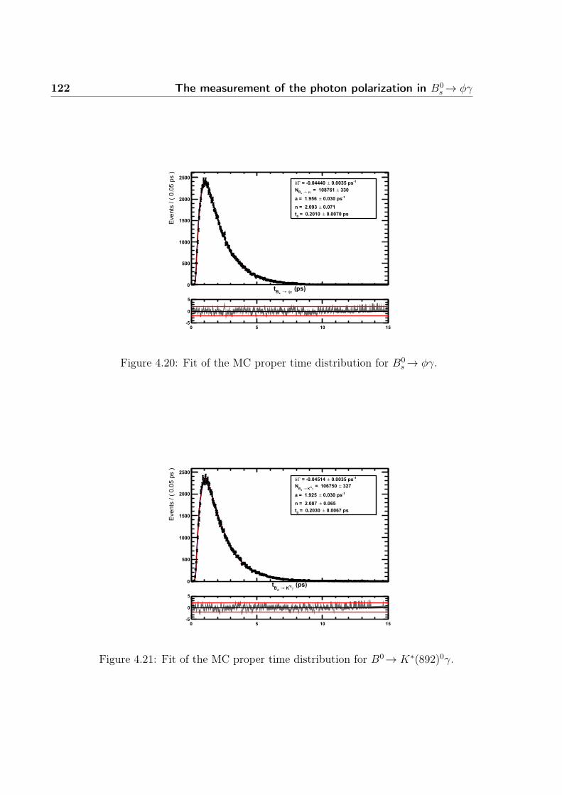
122 The measurement of the photon polarization in B0s → φγ
�����γφ�→��*
�
�����������#'#,�/���
�
���
����
����
����
����%���&��4����±�>�%�&������Γδ
�44�±�>�����5���γφ�→��*�
%���&�4����±��>���&6�����&�5�±��>���&�64���&��5����±�>���&�������
� � �� ��%�
�
�
Figure 4.20: Fit of the MC proper time distribution for B0s → φγ.
�����γ?��@→�'*
�
�����������#'#,�/���
�
���
����
����
����
����%���&��4����±�>�%�&������Γδ
�4�5±�>�����5���γ?��@→�'*
�%���&�4����±��>���&6���
��&���±��>���&��5���&���5���±�>���&��4����
� � �� ��%�
�
�
Figure 4.21: Fit of the MC proper time distribution for B0→ K∗(892)0γ.
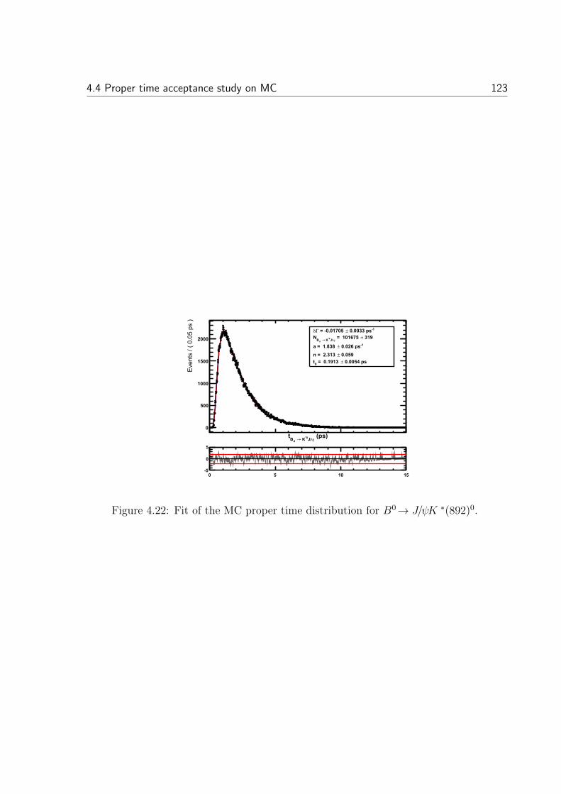
4.4 Proper time acceptance study on MC 123
�����ψ=)?��@→�'*
�
�����������#'#,�/���
�
���
����
����
����
%���&��44���±�>�%�&��5���Γδ�4�6±�>������5��
ψ=)?��@→�'*�
%���&������±��>���&�4����&��6±��>���&4�4���&�������±�>���&�6�4���
� � �� ��%�
�
�
Figure 4.22: Fit of the MC proper time distribution for B0→ J/ψK ∗(892)0.
124 The measurement of the photon polarization in B0s → φγ
4.4.3 Acceptance at high proper time introduced by the trigger
The global δΓ obtained fitting the proper time distributions on MC is ∼ 30 ns−1 for theB0 → J/ψX sample and ∼ 40 ns−1 for the radiative samples (see section 4.4.2). Thissection addresses a study of the proper time acceptance introduced at high proper time(> 2 ps) by the trigger. The main sources of inefficiency at high decay times comesfrom VELO geometrical acceptance and the reconstruction of tracks.
4.4.3.1 MC study
Using B0s → φγ, B0 → K∗(892)0γ, B0 → J/ψK ∗(892)0 or B0
s → J/ψφ MC sam-ples, the ratio of the proper time distribution with one specific trigger line appliedplus the offline selection over the proper time distribution with only the offline selec-tion applied is done. For each step of the trigger path this ratio is fitted startingfrom 2 ps with an exponential of the form e−δΓtriggerX.t where the term δΓtriggerX =
δΓ(trigger X+offline selection) − δΓ(offline selection) parametrizes the relative proper time accep-tance at high proper time induced by this specific trigger line.Figure 4.23 shows the ratio of the proper time distributions obtained from B0
s → φγ MCevents. Table 4.11 reports the values of the δΓtriggerX fitted on B0
s → φγ, B0→ K∗(892)0γ,B0→ J/ψK ∗(892)0 and B0
s → J/ψφ MC for different trigger criteria. As expected, theL0 tripper does not introduce any high proper time acceptance. The HLT2 containscuts that affect the acceptance at high proper time but the HLT2 event reconstructionis relatively close to the offline one and those cuts are already present in the offline selec-tion. Hence, the relative effect of the HLT2 with respect to the offline selection is verymodest. On the other hand, because the HLT1 tracking is different from the offline one,the HLT1 introduces a significant inefficiency at high proper time even relatively to theoffline selection. The overall δΓHLT1 introduced by the HLT1, or δΓtrigger introduced bythe whole trigger given that HLT1 fully dominates here, is similar for the three samples,and is of the order of 20 ns−1 for B0
s → φγ and 10 ns−1 for B0 → K∗(892)0γ and thedi-muon channels.
It has been shown in an other analysis [106] that about half of the acceptance slopeintroduced by the HLT1 TOS trigger requirement is related to a drop of the VELOreconstruction efficiency for tracks that are significantly displaced with respect to thebeam axis. This inefficiency has been exhaustively studied for the B(Λb) → J/ψX
lifetime measurements [106]. The VELO reconstruction is done by the FastVelo algo-
4.4 Proper time acceptance study on MC 125
rithm [107] with different online and offline versions. A detailed description can be foundin [108]. The track finding procedure assumes that tracks originate approximately fromthe beam line. The VELO track reconstruction efficiency depends also on the eventtrack multiplicity and pT of the track. The effect is even worse in the case of the φ
meson reconstruction because of the small opening angle between its decay products.Moreover, the Hlt1TrackAllL0 lines used in this analysis have additional requirements inthe minimum number of VELO hits and T hits of the reconstructed tracks that are notapplied for instance in the Hlt1DiMuon lines. These additional requirements, togetherwith the pT requirement on the track, modify further the acceptance.
4.4.3.2 Crosscheck on data
Since the HLT1TrackAllL0 TOS (applied only on the K∗(φ) decay products for B0 →K∗(892)0γ (B0
s → φγ)) is not required in the di-muon trigger and stripping, its effectcan be checked on data. Figure 4.24 show the ratio of the proper time distributionfor this trigger requirement with respect to the offline selection as obtained for theB0→ J/ψK ∗(892)0 data events. The fitted δΓHLT1TrackAllL0−TOS is 13.3 ± 4.4 ns−1 whichis compatible with 5.0± 2.4 ns−1 obtained from the simulation. The same check is per-formed on B0
s → J/ψφ, the obtained value for δΓHLT1TrackAllL0−TOS is −9.2 ± 12.4 ns−1
which is compatible with 7.7 ± 2.1 ns−1 obtained from simulation. Those results arereported in Table 4.12.
To conclude on this, it has been shown that, relative to the offline selection, only theHLT1 has a significant effect on the high proper time acceptance and it has been checkedthat for B0→ J/ψX the simulation reproduces in the limit of statistical uncertainty theeffect of the HLT1TrackAllL0-TOS.
4.4.4 Proper time distribution of control samples in data
Independent fit to the proper time distributions of B0→ K∗(892)0γ and B0→ J/ψK ∗(892)0
are performed on data. The physical lifetimes of the B0 meson are fixed to the latestworld average τB0 = 1.520± 0.004 ps [96]. The result are shown in table 4.13. The ac-ceptance at low proper time for B0→ K∗(892)0γ and B0→ J/ψK ∗(892)0 are consistentwithin errors thanks to the dedicated weighing and cut scaling procedure. From this itcan be deduced that B0→ J/ψK ∗(892)0 can be used in the data fit so as to constraintthe acceptance at low proper time of the radiative channels.
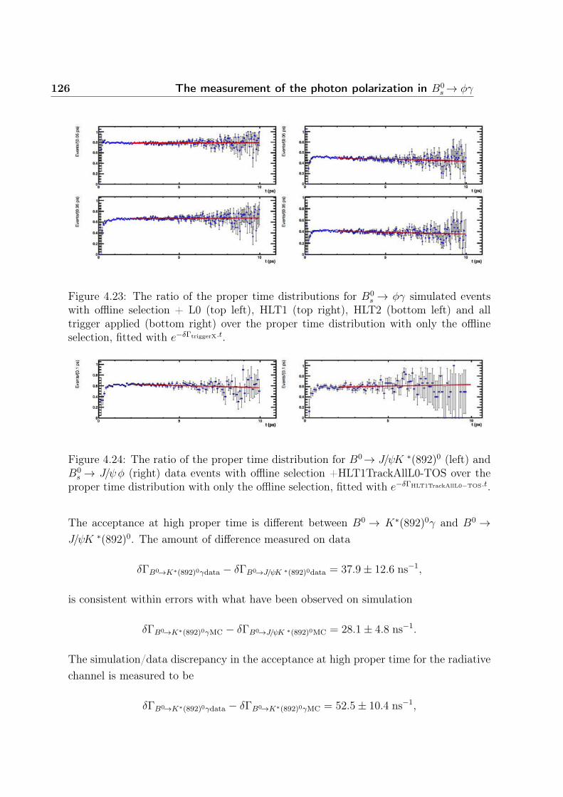
126 The measurement of the photon polarization in B0s → φγ
Figure 4.23: The ratio of the proper time distributions for B0s → φγ simulated events
with offline selection + L0 (top left), HLT1 (top right), HLT2 (bottom left) and alltrigger applied (bottom right) over the proper time distribution with only the offlineselection, fitted with e−δΓtriggerX.t.
Figure 4.24: The ratio of the proper time distribution for B0→ J/ψK ∗(892)0 (left) andB0
s → J/ψφ (right) data events with offline selection +HLT1TrackAllL0-TOS over theproper time distribution with only the offline selection, fitted with e−δΓHLT1TrackAllL0−TOS.t.
The acceptance at high proper time is different between B0 → K∗(892)0γ and B0 →J/ψK ∗(892)0. The amount of difference measured on data
δΓB0→K∗(892)0γdata − δΓB0→J/ψK ∗(892)0data = 37.9± 12.6 ns−1,
is consistent within errors with what have been observed on simulation
δΓB0→K∗(892)0γMC − δΓB0→J/ψK ∗(892)0MC = 28.1± 4.8 ns−1.
The simulation/data discrepancy in the acceptance at high proper time for the radiativechannel is measured to be
δΓB0→K∗(892)0γdata − δΓB0→K∗(892)0γMC = 52.5± 10.4 ns−1,
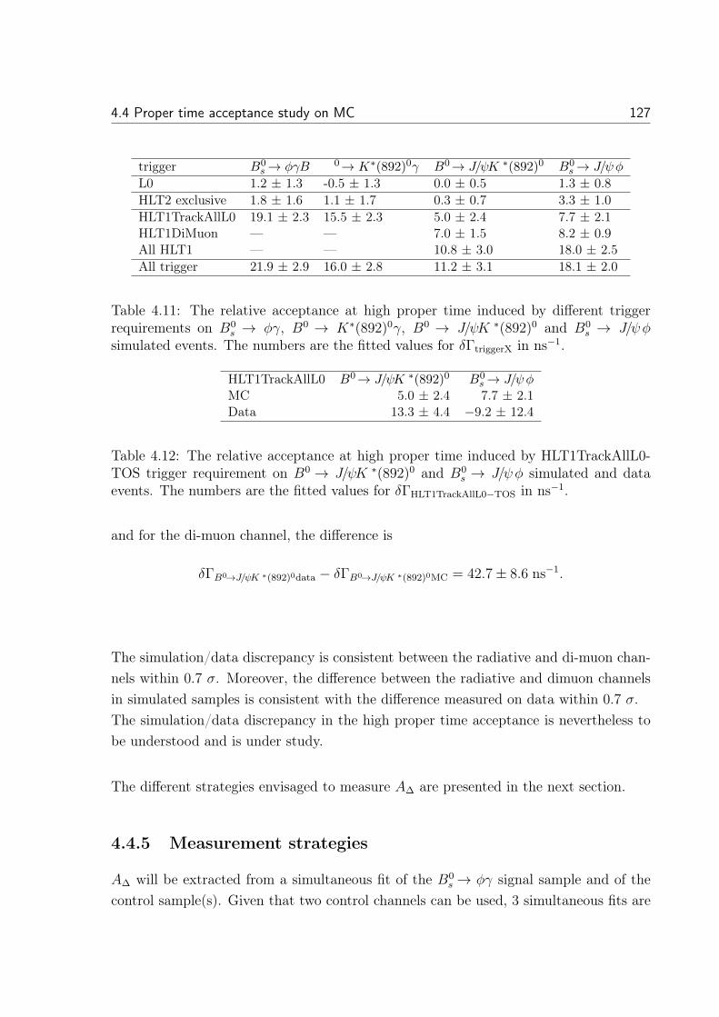
4.4 Proper time acceptance study on MC 127
trigger B0s → φγB 0→ K∗(892)0γ B0→ J/ψK ∗(892)0 B0
s → J/ψφ
L0 1.2 ± 1.3 -0.5 ± 1.3 0.0 ± 0.5 1.3 ± 0.8HLT2 exclusive 1.8 ± 1.6 1.1 ± 1.7 0.3 ± 0.7 3.3 ± 1.0HLT1TrackAllL0 19.1 ± 2.3 15.5 ± 2.3 5.0 ± 2.4 7.7 ± 2.1HLT1DiMuon — — 7.0 ± 1.5 8.2 ± 0.9All HLT1 — — 10.8 ± 3.0 18.0 ± 2.5All trigger 21.9 ± 2.9 16.0 ± 2.8 11.2 ± 3.1 18.1 ± 2.0
Table 4.11: The relative acceptance at high proper time induced by different triggerrequirements on B0
s → φγ, B0 → K∗(892)0γ, B0 → J/ψK ∗(892)0 and B0s → J/ψφ
simulated events. The numbers are the fitted values for δΓtriggerX in ns−1.
HLT1TrackAllL0 B0→ J/ψK ∗(892)0 B0s → J/ψφ
MC 5.0 ± 2.4 7.7 ± 2.1Data 13.3 ± 4.4 −9.2 ± 12.4
Table 4.12: The relative acceptance at high proper time induced by HLT1TrackAllL0-TOS trigger requirement on B0 → J/ψK ∗(892)0 and B0
s → J/ψφ simulated and dataevents. The numbers are the fitted values for δΓHLT1TrackAllL0−TOS in ns−1.
and for the di-muon channel, the difference is
δΓB0→J/ψK ∗(892)0data − δΓB0→J/ψK ∗(892)0MC = 42.7± 8.6 ns−1.
The simulation/data discrepancy is consistent between the radiative and di-muon chan-nels within 0.7 σ. Moreover, the difference between the radiative and dimuon channelsin simulated samples is consistent with the difference measured on data within 0.7 σ.The simulation/data discrepancy in the high proper time acceptance is nevertheless tobe understood and is under study.
The different strategies envisaged to measure AΔ are presented in the next section.
4.4.5 Measurement strategies
AΔ will be extracted from a simultaneous fit of the B0s → φγ signal sample and of the
control sample(s). Given that two control channels can be used, 3 simultaneous fits are
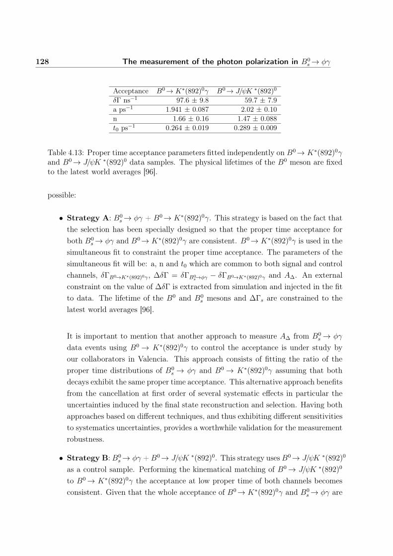
128 The measurement of the photon polarization in B0s → φγ
Acceptance B0→ K∗(892)0γ B0→ J/ψK ∗(892)0
δΓ ns−1 97.6 ± 9.8 59.7 ± 7.9a ps−1 1.941 ± 0.087 2.02 ± 0.10n 1.66 ± 0.16 1.47 ± 0.088t0 ps−1 0.264 ± 0.019 0.289 ± 0.009
Table 4.13: Proper time acceptance parameters fitted independently on B0→ K∗(892)0γand B0→ J/ψK ∗(892)0 data samples. The physical lifetimes of the B0 meson are fixedto the latest world averages [96].
possible:
• Strategy A: B0s → φγ + B0→ K∗(892)0γ. This strategy is based on the fact that
the selection has been specially designed so that the proper time acceptance forboth B0
s → φγ and B0→ K∗(892)0γ are consistent. B0→ K∗(892)0γ is used in thesimultaneous fit to constraint the proper time acceptance. The parameters of thesimultaneous fit will be: a, n and t0 which are common to both signal and controlchannels, δΓB0→K∗(892)0γ, ΔδΓ = δΓB0
s→φγ − δΓB0→K∗(892)0γ and AΔ. An externalconstraint on the value of ΔδΓ is extracted from simulation and injected in the fitto data. The lifetime of the B0 and B0
s mesons and ΔΓs are constrained to thelatest world averages [96].
It is important to mention that another approach to measure AΔ from B0s → φγ
data events using B0 → K∗(892)0γ to control the acceptance is under study byour collaborators in Valencia. This approach consists of fitting the ratio of theproper time distributions of B0
s → φγ and B0 → K∗(892)0γ assuming that bothdecays exhibit the same proper time acceptance. This alternative approach benefitsfrom the cancellation at first order of several systematic effects in particular theuncertainties induced by the final state reconstruction and selection. Having bothapproaches based on different techniques, and thus exhibiting different sensitivitiesto systematics uncertainties, provides a worthwhile validation for the measurementrobustness.
• Strategy B: B0s → φγ + B0→ J/ψK ∗(892)0. This strategy uses B0→ J/ψK ∗(892)0
as a control sample. Performing the kinematical matching of B0→ J/ψK ∗(892)0
to B0→ K∗(892)0γ the acceptance at low proper time of both channels becomesconsistent. Given that the whole acceptance of B0→ K∗(892)0γ and B0
s → φγ are
4.4 Proper time acceptance study on MC 129
consistent, the acceptance at low proper time of B0s → φγ and B0→ J/ψK ∗(892)0
are also consistent. The difference between the acceptance at high proper time,ΔδΓ = δΓB0
s→φγ−δΓB0→J/ψK ∗(892)0 , is obtained from the study on simulated events.If the differences in the proper time acceptance between the simulation and dataare well understood, the difference ΔδΓ from simulation is applied in the data fitas an external constraint in the simultaneous fit. The parameters of the simulta-neous fit will be: a, n and t0 which are common to both channels, δΓB0→J/ψK ∗(892)0 ,ΔδΓ = δΓB0
s→φγ − δΓB0→J/ψK ∗(892)0 and AΔ. An external constraint on the valueof ΔδΓ is extracted from simulation and injected in the fit to data. The lifetimeof the B0 and B0
s mesons and ΔΓs are constrained to the latest world averages [96].
• Strategy C: B0s → φγ + B0 → K∗(892)0γ + B0 → J/ψK ∗(892)0. This strategy
uses both B0 → K∗(892)0γ and B0 → J/ψK ∗(892)0 as control samples. It takesinto account the fact that the radiative decays have consistent acceptances bothat low and high proper times. The acceptance at low proper time is consistent forthe three channels. For strategy C, two options are possible.
– B0 → J/ψK ∗(892)0 is used only to constraint the acceptance at low propertime and B0 → K∗(892)0γ is used to constrain the acceptance of B0
s → φγ.The parameters of the simultaneous fit will be: a, n, t0 which are commonto the three channels, δΓB0→K∗(892)0γ, δΓB0→J/ψK ∗(892)0 , ΔδΓ = δΓB0
s→φγ −δΓB0→K∗(892)0γ and AΔ. An external constraint on the value of ΔδΓ is ex-tracted from simulation and injected in the fit to data. The lifetime of theB0 and B0
s mesons and ΔΓs are constrained to the latest world averages [96].
– Both B0 → K∗(892)0γ and B0 → J/ψK ∗(892)0 can be used to constrainthe acceptance at low proper time and the acceptance at high proper timewith a constraint on the difference ΔδΓ = δΓB0
s→φγ − δΓB0→K∗(892)0γ andΔδΓ = δΓB0→K∗(892)0γ − δΓB0→J/ψK ∗(892)0 that are extracted from simulation.The parameters of the simultaneous fit will be: a, n, t0 which are commonto the three channels, δΓB0→J/ψK ∗(892)0 , ΔδΓ = δΓB0
s→φγ − δΓB0→K∗(892)0γ,ΔδΓ = δΓB0→K∗(892)0γ − δΓB0→J/ψK ∗(892)0 and AΔ. An external constraint onthe values of both ΔδΓ is extracted from simulation and injected in the fit todata. The lifetime of the B0 and B0
s mesons and ΔΓs are constrained to thelatest world averages [96].

130 The measurement of the photon polarization in B0s → φγ
The choice between the strategies to measure AΔ will be decided after all the system-atics are evaluated. If one control sample happens to have much smaller systematicuncertainties than the other it will in fact be better to only use this control sample. Thestrategies are discussed in details in chapter 5.

Chapter 5
Preliminary results
Contents5.1 Fit strategies . . . . . . . . . . . . . . . . . . . . . . . . . . . . 132
5.2 Extracting τB0 with B0→ K∗(892)0γ events . . . . . . . . . . . 135
5.3 Sensitivity on AΔ . . . . . . . . . . . . . . . . . . . . . . . . . . 141
5.3.1 Strategy A . . . . . . . . . . . . . . . . . . . . . . . . . . . . . 141
5.3.2 Strategy B . . . . . . . . . . . . . . . . . . . . . . . . . . . . . 144
5.3.3 Strategy C1 . . . . . . . . . . . . . . . . . . . . . . . . . . . . . 147
5.3.4 Strategy C2 . . . . . . . . . . . . . . . . . . . . . . . . . . . . . 150
5.3.5 Summary . . . . . . . . . . . . . . . . . . . . . . . . . . . . . . 153
5.4 Systematic uncertainties study . . . . . . . . . . . . . . . . . 153
5.4.1 Background contamination and modeling . . . . . . . . . . . . 154
5.4.2 External physical inputs . . . . . . . . . . . . . . . . . . . . . . 157
5.4.3 Scaling and weighing procedure . . . . . . . . . . . . . . . . . . 158
5.4.4 Other systematics . . . . . . . . . . . . . . . . . . . . . . . . . 160
5.5 Conclusions . . . . . . . . . . . . . . . . . . . . . . . . . . . . . 161
131
132 Preliminary results
The control of the proper time acceptance is the major difficulty in the precisedetermination of the photon polarization. It has been intensively discussed in chapter4. The events selection has been specially designed to keep consistent the proper timeacceptance between B0 → K∗(892)0γ and B0
s → φγ. To control the B0 → K∗(892)0γ
acceptance with the B0→ J/ψK ∗(892)0 mode, a dedicated weighing and scaling procedurehas been setup and is discussed in 4.4.1. B0→ K∗(892)0γ and B0→ J/ψK ∗(892)0 arehenceforth two possible control samples for the proper time acceptance in B0
s → φγ.This chapter introduces the preliminary results for the extraction of AΔ. First, the fitstrategies with the different control samples are discussed in section 5.1. A validation ofthe fitting procedure is done by measuring the B0 lifetime from B0→ K∗(892)0γ signalevents using B0 → J/ψK ∗(892)0 as a control sample, this is reported in section 5.2.Section 5.3 shows the preliminary fits for the different strategies presented along withthe preliminary results obtained for AΔ. The central value of AΔ is not shown waitingfor the analysis to be finalized and only the measured statistical uncertainty is discussed.Section 5.4 addresses the systematic uncertainties and section 5.5 gives the concludingremarks.
5.1 Fit strategies
As discussed in 4.4.5, three strategies can be set up to extract AΔ:
• Strategy A: B0→ K∗(892)0γ is used as a control sample.
• Strategy B: B0→ J/ψK ∗(892)0 is used as a control sample.
• Strategy C: B0 → K∗(892)0γ and B0 → J/ψK ∗(892)0 are both used as controlsamples.
– C1: B0 → J/ψK ∗(892)0 is used to constrain the acceptance at low propertime.
– C2: B0 → J/ψK ∗(892)0 is used to constrain both the acceptance at lowand high proper time. For the difference in the acceptance at high propertime, external constraints extracted from simulation are used in the data fits.This approach requires that possible differences in the acceptance betweensimulation and data are understood and well under control.
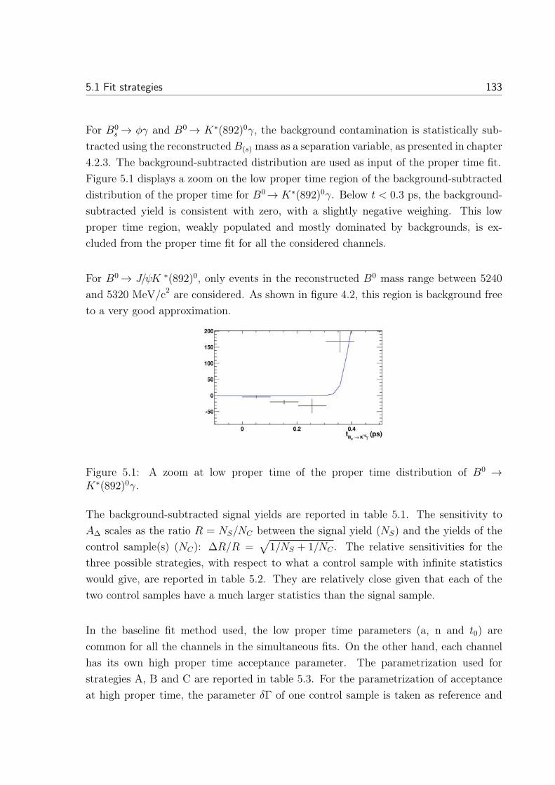
5.1 Fit strategies 133
For B0s → φγ and B0 → K∗(892)0γ, the background contamination is statistically sub-
tracted using the reconstructed B(s) mass as a separation variable, as presented in chapter4.2.3. The background-subtracted distribution are used as input of the proper time fit.Figure 5.1 displays a zoom on the low proper time region of the background-subtracteddistribution of the proper time for B0→ K∗(892)0γ. Below t < 0.3 ps, the background-subtracted yield is consistent with zero, with a slightly negative weighing. This lowproper time region, weakly populated and mostly dominated by backgrounds, is ex-cluded from the proper time fit for all the considered channels.
For B0 → J/ψK ∗(892)0, only events in the reconstructed B0 mass range between 5240and 5320 MeV/c2 are considered. As shown in figure 4.2, this region is background freeto a very good approximation.
Figure 5.1: A zoom at low proper time of the proper time distribution of B0 →K∗(892)0γ.
The background-subtracted signal yields are reported in table 5.1. The sensitivity toAΔ scales as the ratio R = NS/NC between the signal yield (NS) and the yields of thecontrol sample(s) (NC): ΔR/R =
√1/NS + 1/NC . The relative sensitivities for the
three possible strategies, with respect to what a control sample with infinite statisticswould give, are reported in table 5.2. They are relatively close given that each of thetwo control samples have a much larger statistics than the signal sample.
In the baseline fit method used, the low proper time parameters (a, n and t0) arecommon for all the channels in the simultaneous fits. On the other hand, each channelhas its own high proper time acceptance parameter. The parametrization used forstrategies A, B and C are reported in table 5.3. For the parametrization of acceptanceat high proper time, the parameter δΓ of one control sample is taken as reference and

134 Preliminary results
B0s → φγB 0→ K∗(892)0γ B0→ J/ψK ∗(892)0
3.5 103 24 103 30 103
Table 5.1: Selected signal yields for t>0.3 ps. Background subtraction is applied for theradiative modes.
NC → ∞ A B C1 1.071 1.058 1.032
Table 5.2: Relative sensitivities on AΔ from the different strategies for the control sam-ple(s).
the difference, ΔδΓ = δΓx − δΓRef , is (are) used for the other sample(s). For eachstrategy, the simultaneous fit is first performed on simulated events to extract the ΔδΓ
parameter(s). The ΔδΓ obtained from the simulation is (are) then used as an externalgaussian constraint(s) of the simultaneous fit on data. The constraint
ΔδΓ2 = δΓB0s→φγ − δΓB0→K∗(892)0γ = 3.0± 2.9 ns−1
is used in strategies A, C1 and C2, the constraint
ΔδΓ3 = δΓB0s→φγ − δΓB0→J/ψK ∗(892)0 = 36.0± 2.9 ns−1
is used in strategy B and the constraint
ΔδΓ1 = ΔδΓ3 −ΔδΓ2 = δΓB0→K∗(892)0γ − δΓB0→J/ψK ∗(892)0 = 32.8± 3.0 ns−1
is used, along with ΔδΓ2 in strategy C2. In strategy C2, the correlation between ΔδΓ1
and ΔδΓ2 values is taken into account using the covariance matrix from the fit on thesimulated samples.
The above parametrization of the simultaneous fit considers the parameters a, n and t0,that models the acceptance at low proper time, as being common to both the B0
s → φγ
signal and the control(s) channel(s). This is supported by the analysis of simulated datapresented in 4.4.2. In order to evaluate the impact of this strong constraint on the mea-surement, an alternative parametrization of the simultaneous fits has been defined. Asin the baseline approach, the a and n parameters of the acceptance at low proper timeare common for all the samples considered in the simultaneous fit, while the t0 parameter
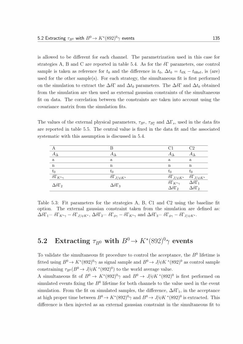
5.2 Extracting τB0 with B0→ K∗(892)0γ events 135
is allowed to be different for each channel. The parametrization used in this case forstrategies A, B and C are reported in table 5.4. As for the δΓ parameters, one controlsample is taken as reference for t0 and the difference in t0, Δt0 = t0X − t0Ref , is (are)used for the other sample(s). For each strategy, the simultaneous fit is first performedon the simulation to extract the ΔδΓ and Δt0 parameters. The ΔδΓ and Δt0 obtainedfrom the simulation are then used as external gaussian constraints of the simultaneousfit on data. The correlation between the constraints are taken into account using thecovariance matrix from the simulation fits.
The values of the external physical parameters, τB0 , τB0s
and ΔΓs, used in the data fitsare reported in table 5.5. The central value is fixed in the data fit and the associatedsystematic with this assumption is discussed in 5.4.
A B C1 C2AΔ AΔ AΔ AΔ
a a a an n n nt0 t0 t0 t0δΓK∗γ δΓJ/ψK∗ δΓJ/ψK∗ δΓJ/ψK∗
ΔδΓ2 ΔδΓ3δΓK∗γ ΔδΓ1
ΔδΓ2 ΔδΓ2
Table 5.3: Fit parameters for the strategies A, B, C1 and C2 using the baseline fitoption. The external gaussian constraint taken from the simulation are defined as:ΔδΓ1= δΓK∗γ − δΓJ/ψK∗ , ΔδΓ2= δΓφγ − δΓK∗γ and ΔδΓ3= δΓφγ − δΓJ/ψK∗ .
5.2 Extracting τB0 with B0→ K∗(892)0γ events
To validate the simultaneous fit procedure to control the acceptance, the B0 lifetime isfitted using B0→ K∗(892)0γ as signal sample and B0→ J/ψK ∗(892)0 as control sampleconstraining τB0(B0→ J/ψK ∗(892)0) to the world average value.A simultaneous fit of B0 → K∗(892)0γ and B0 → J/ψK ∗(892)0 is first performed onsimulated events fixing the B0 lifetime for both channels to the value used in the eventsimulation. From the fit on simulated samples, the difference, ΔδΓ1, in the acceptanceat high proper time between B0→ K∗(892)0γ and B0→ J/ψK ∗(892)0 is extracted. Thisdifference is then injected as an external gaussian constraint in the simultaneous fit to
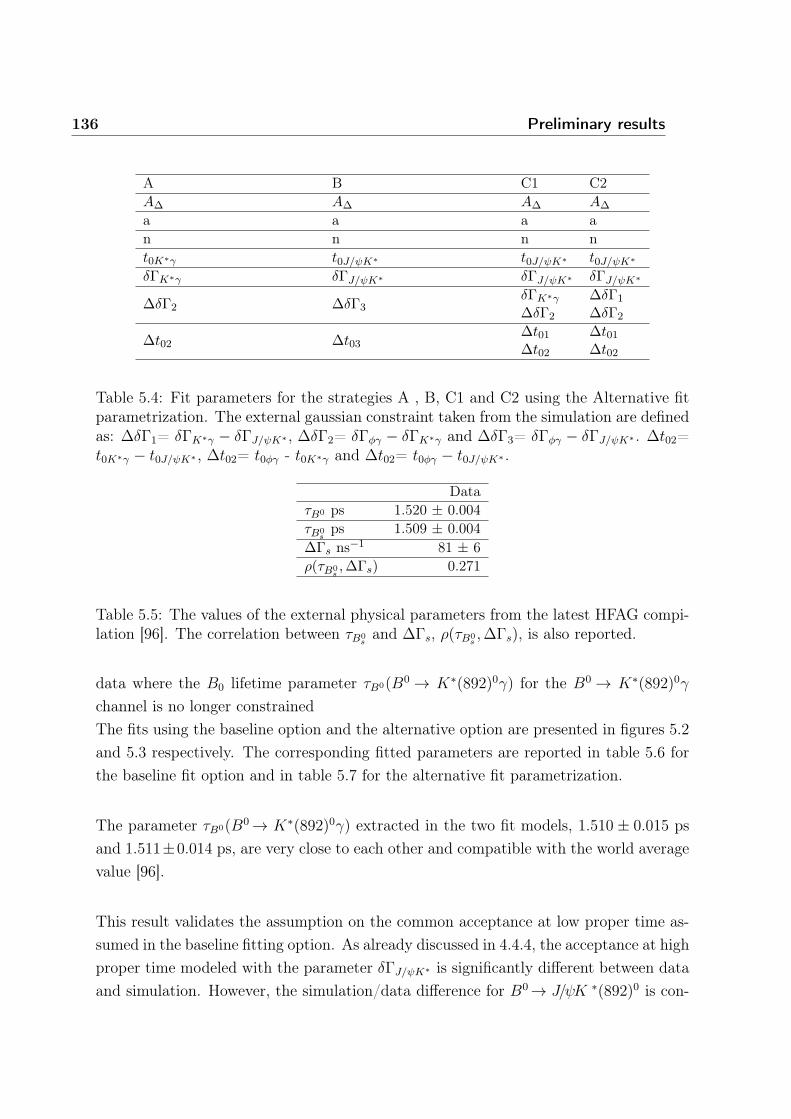
136 Preliminary results
A B C1 C2AΔ AΔ AΔ AΔ
a a a an n n nt0K∗γ t0J/ψK∗ t0J/ψK∗ t0J/ψK∗
δΓK∗γ δΓJ/ψK∗ δΓJ/ψK∗ δΓJ/ψK∗
ΔδΓ2 ΔδΓ3δΓK∗γ ΔδΓ1
ΔδΓ2 ΔδΓ2
Δt02 Δt03Δt01 Δt01Δt02 Δt02
Table 5.4: Fit parameters for the strategies A , B, C1 and C2 using the Alternative fitparametrization. The external gaussian constraint taken from the simulation are definedas: ΔδΓ1= δΓK∗γ − δΓJ/ψK∗ , ΔδΓ2= δΓφγ − δΓK∗γ and ΔδΓ3= δΓφγ − δΓJ/ψK∗ . Δt02=t0K∗γ − t0J/ψK∗ , Δt02= t0φγ - t0K∗γ and Δt02= t0φγ − t0J/ψK∗ .
DataτB0 ps 1.520 ± 0.004τB0
sps 1.509 ± 0.004
ΔΓs ns−1 81 ± 6ρ(τB0
s,ΔΓs) 0.271
Table 5.5: The values of the external physical parameters from the latest HFAG compi-lation [96]. The correlation between τB0
sand ΔΓs, ρ(τB0
s,ΔΓs), is also reported.
data where the B0 lifetime parameter τB0(B0 → K∗(892)0γ) for the B0 → K∗(892)0γ
channel is no longer constrainedThe fits using the baseline option and the alternative option are presented in figures 5.2and 5.3 respectively. The corresponding fitted parameters are reported in table 5.6 forthe baseline fit option and in table 5.7 for the alternative fit parametrization.
The parameter τB0(B0→ K∗(892)0γ) extracted in the two fit models, 1.510 ± 0.015 psand 1.511±0.014 ps, are very close to each other and compatible with the world averagevalue [96].
This result validates the assumption on the common acceptance at low proper time as-sumed in the baseline fitting option. As already discussed in 4.4.4, the acceptance at highproper time modeled with the parameter δΓJ/ψK∗ is significantly different between dataand simulation. However, the simulation/data difference for B0→ J/ψK ∗(892)0 is con-
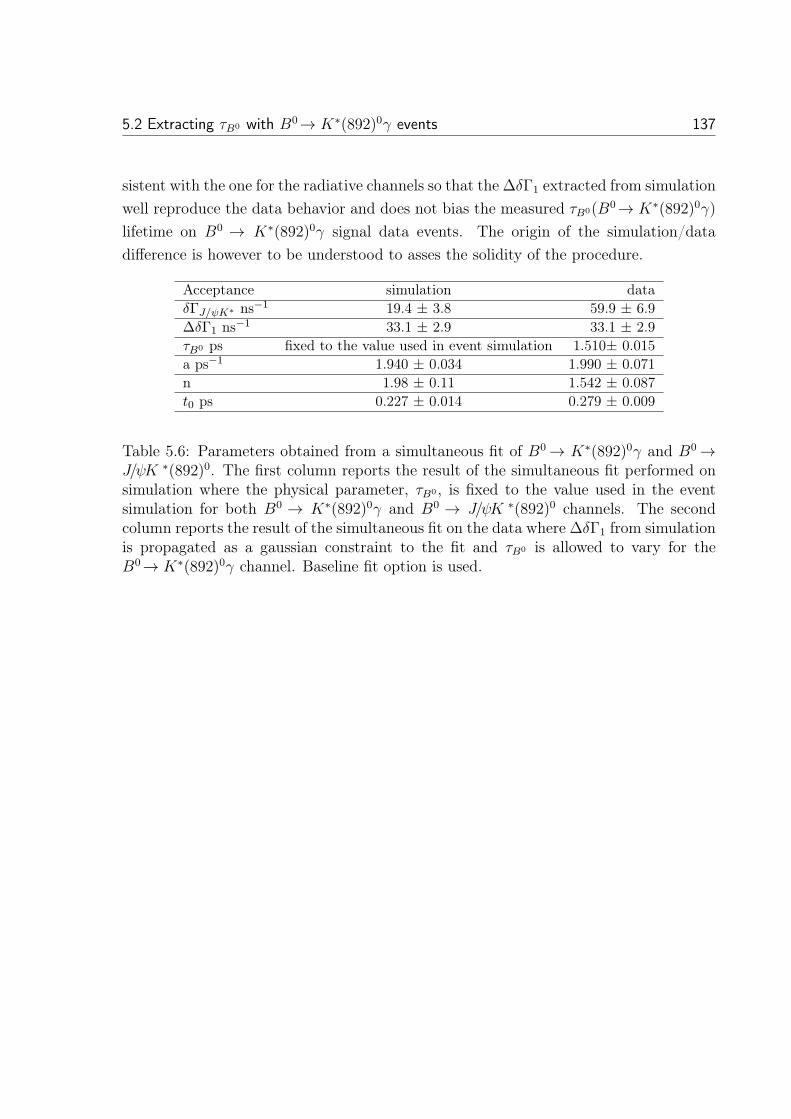
5.2 Extracting τB0 with B0→ K∗(892)0γ events 137
sistent with the one for the radiative channels so that the ΔδΓ1 extracted from simulationwell reproduce the data behavior and does not bias the measured τB0(B0→ K∗(892)0γ)lifetime on B0 → K∗(892)0γ signal data events. The origin of the simulation/datadifference is however to be understood to asses the solidity of the procedure.
Acceptance simulation dataδΓJ/ψK∗ ns−1 19.4 ± 3.8 59.9 ± 6.9ΔδΓ1 ns−1 33.1 ± 2.9 33.1 ± 2.9τB0 ps fixed to the value used in event simulation 1.510± 0.015a ps−1 1.940 ± 0.034 1.990 ± 0.071n 1.98 ± 0.11 1.542 ± 0.087t0 ps 0.227 ± 0.014 0.279 ± 0.009
Table 5.6: Parameters obtained from a simultaneous fit of B0 → K∗(892)0γ and B0 →J/ψK ∗(892)0. The first column reports the result of the simultaneous fit performed onsimulation where the physical parameter, τB0 , is fixed to the value used in the eventsimulation for both B0 → K∗(892)0γ and B0 → J/ψK ∗(892)0 channels. The secondcolumn reports the result of the simultaneous fit on the data where ΔδΓ1 from simulationis propagated as a gaussian constraint to the fit and τB0 is allowed to vary for theB0→ K∗(892)0γ channel. Baseline fit option is used.
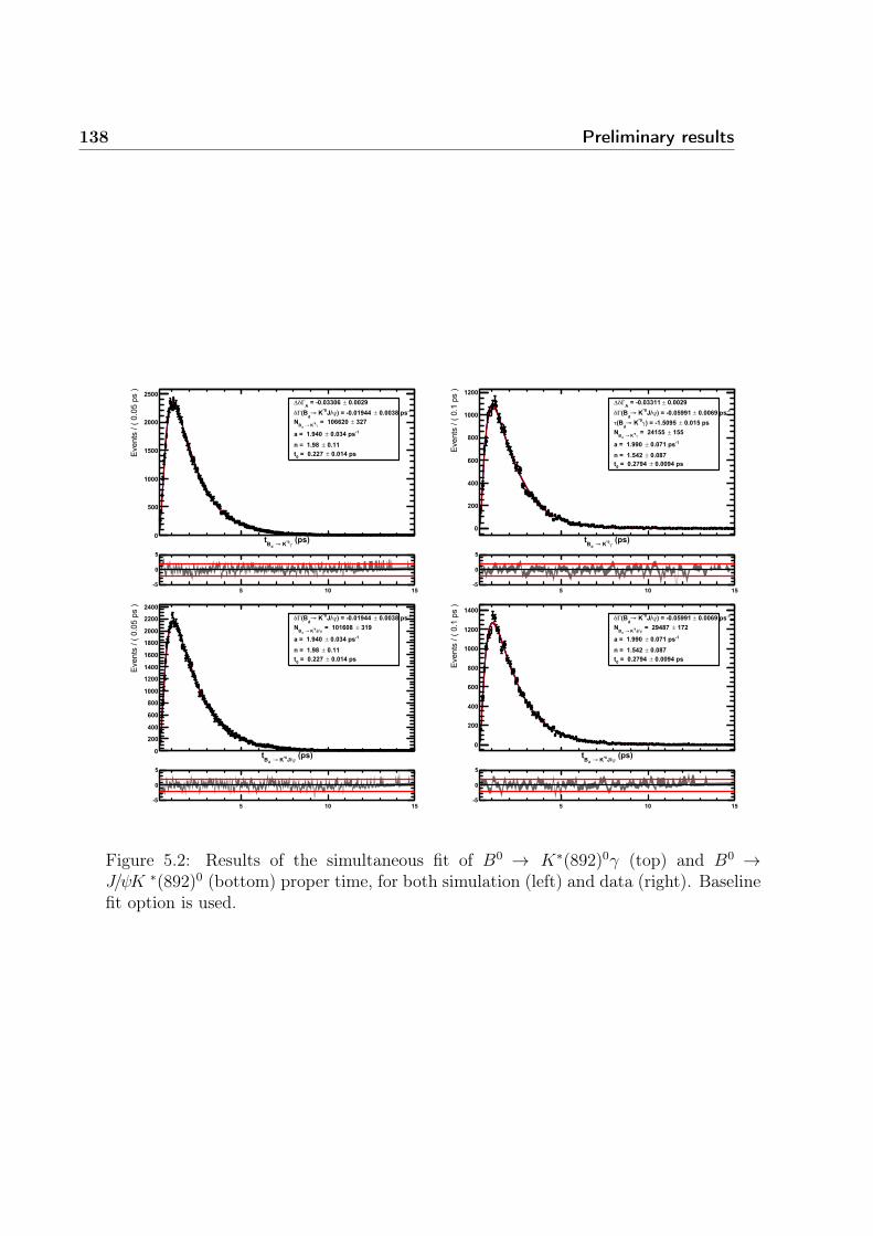
138 Preliminary results
�����γ?��@→�'*
�
�����������#'#,�/���
�
���
����
����
����
������&���6±�>�%�&�44���3ΓδΔ
%���&��4����±��>�%�&��6���ψ=)?��@→'
�*Γδ
�4�5±�>���������γ?��@→�'*
�%���&�4����±��>���&6���
��&��±��>���&6����&������±�>���&��5���
� �� ��%�
�
�
�����γ?��@→�'*
�
�����������#'"�/���
�
���
���
���
���
����
������&���6±�>�%�&�44���3ΓδΔ
%���&���6���±��>�%�&��66��ψ=)?��@→'
�*Γδ
��&������±��>�%�&��6��γ?��@→'
�*τ����±�>��������
γ?��@→�'*�
%���&�5����±��>���&66����&��5±��>���&������&��6����±�>���&�56����
� �� ��%�
�
�
�����ψ=)?��@→�'*
�
�����������#'#,�/���
�
���
���
���
���
����
����
����
����
����
����
����
����%���&��4����±��>�%�&��6���ψ=)?��@→
'�*Γδ
�4�6±�>���������ψ=)?��@→�'*
�%���&�4����±��>���&6���
��&��±��>���&6����&������±�>���&��5���
� �� ��%�
�
�
�����ψ=)?��@→�'*
�
�����������#'"�/���
�
���
���
���
���
����
����
����%���&���6���±��>�%�&��66��ψ=)?��@→
'�*Γδ
��5�±�>���6��5�ψ=)?��@→�'*
�%���&�5����±��>���&66��
��&��5±��>���&������&��6����±�>���&�56����
� �� ��%�
�
�
Figure 5.2: Results of the simultaneous fit of B0 → K∗(892)0γ (top) and B0 →J/ψK ∗(892)0 (bottom) proper time, for both simulation (left) and data (right). Baselinefit option is used.
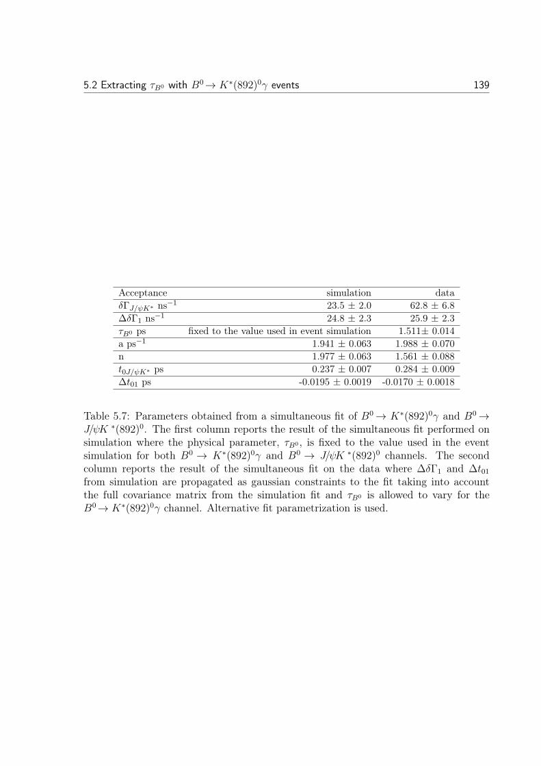
5.2 Extracting τB0 with B0→ K∗(892)0γ events 139
Acceptance simulation dataδΓJ/ψK∗ ns−1 23.5 ± 2.0 62.8 ± 6.8ΔδΓ1 ns−1 24.8 ± 2.3 25.9 ± 2.3τB0 ps fixed to the value used in event simulation 1.511± 0.014a ps−1 1.941 ± 0.063 1.988 ± 0.070n 1.977 ± 0.063 1.561 ± 0.088t0J/ψK∗ ps 0.237 ± 0.007 0.284 ± 0.009Δt01 ps -0.0195 ± 0.0019 -0.0170 ± 0.0018
Table 5.7: Parameters obtained from a simultaneous fit of B0 → K∗(892)0γ and B0 →J/ψK ∗(892)0. The first column reports the result of the simultaneous fit performed onsimulation where the physical parameter, τB0 , is fixed to the value used in the eventsimulation for both B0 → K∗(892)0γ and B0 → J/ψK ∗(892)0 channels. The secondcolumn reports the result of the simultaneous fit on the data where ΔδΓ1 and Δt01from simulation are propagated as gaussian constraints to the fit taking into accountthe full covariance matrix from the simulation fit and τB0 is allowed to vary for theB0→ K∗(892)0γ channel. Alternative fit parametrization is used.
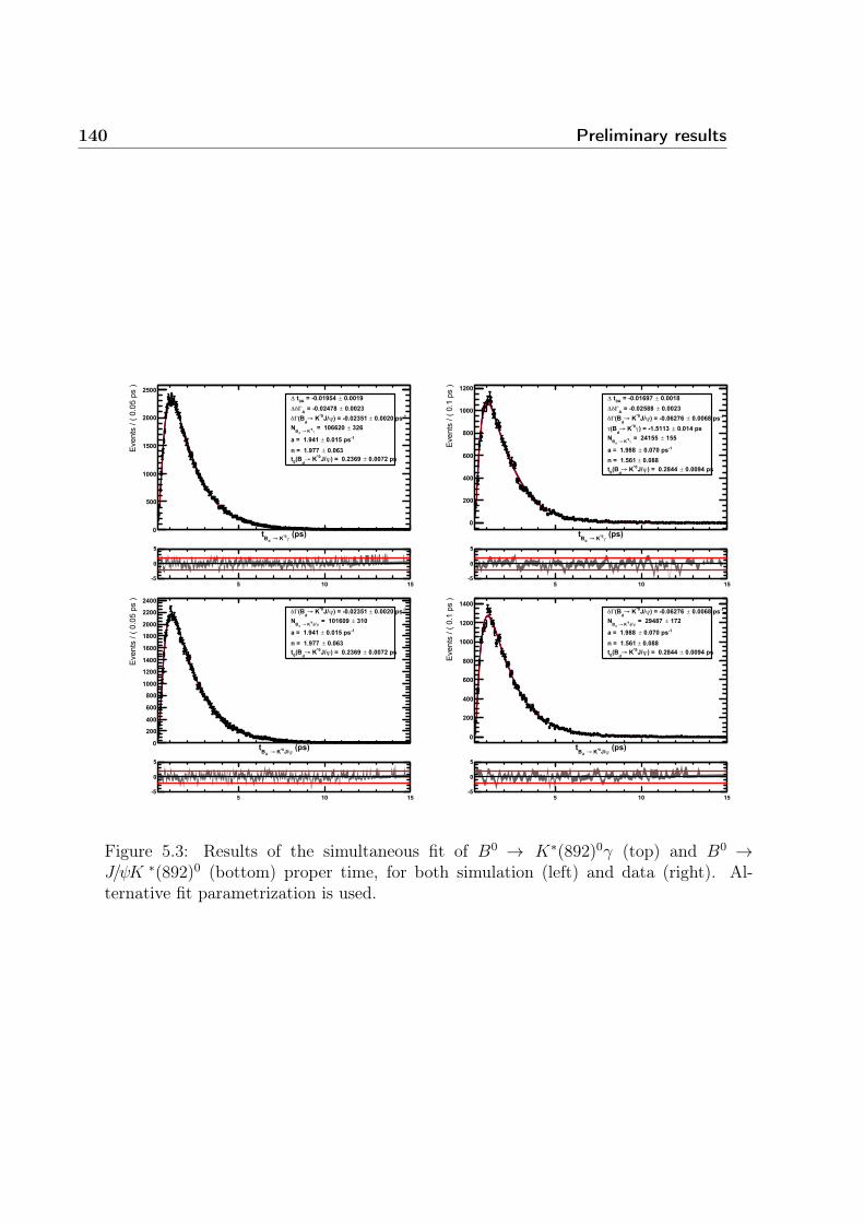
140 Preliminary results
�����γ?��@→�'*
�
�����������#'#,�/���
�
���
����
����
����
������&���6±�>�%�&��6����3��Δ��&���4±�>�%�&���5��3ΓδΔ
%���&�������±��>�%�&��4���ψ=)?��@→'
�*Γδ
�4��±�>���������γ?��@→�'*
�%���&������±��>���&6���
��&��4±��>���&655���&��5����±��>���&�4�6�ψ=)?��@→
'�*��
� �� ��%�
�
�
�����γ?��@→�'*
�
�����������#'"�/���
�
���
���
���
���
����
������&����±�>�%�&���65��3��Δ��&���4±�>�%�&������3ΓδΔ
%���&�������±��>�%�&���5��ψ=)?��@→'
�*Γδ
��&������±��>�%�&���4�γ?��@→'
�*τ����±�>��������
γ?��@→�'*�
%���&�5����±��>���&6�����&���±��>���&����
��&��6����±��>���&�����ψ=)?��@→'
�*��
� �� ��%�
�
�
�����ψ=)?��@→�'*
�
�����������#'#,�/���
�
���
���
���
���
����
����
����
����
����
����
����
����%���&�������±��>�%�&��4���ψ=)?��@→
'�*Γδ
�4��±�>�������6�ψ=)?��@→�'*
�%���&������±��>���&6���
��&��4±��>���&655���&��5����±��>���&�4�6�ψ=)?��@→
'�*��
� �� ��%�
�
�
�����ψ=)?��@→�'*
�
�����������#'"�/���
�
���
���
���
���
����
����
����%���&�������±��>�%�&���5��ψ=)?��@→
'�*Γδ
��5�±�>���6��5�ψ=)?��@→�'*
�%���&�5����±��>���&6���
��&���±��>���&������&��6����±��>���&�����ψ=)?��@→
'�*��
� �� ��%�
�
�
Figure 5.3: Results of the simultaneous fit of B0 → K∗(892)0γ (top) and B0 →J/ψK ∗(892)0 (bottom) proper time, for both simulation (left) and data (right). Al-ternative fit parametrization is used.
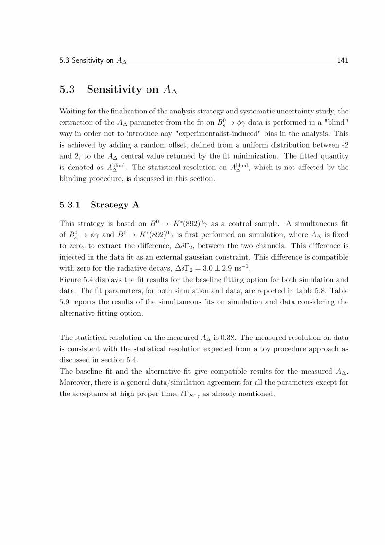
5.3 Sensitivity on AΔ 141
5.3 Sensitivity on AΔ
Waiting for the finalization of the analysis strategy and systematic uncertainty study, theextraction of the AΔ parameter from the fit on B0
s → φγ data is performed in a "blind"way in order not to introduce any "experimentalist-induced" bias in the analysis. Thisis achieved by adding a random offset, defined from a uniform distribution between -2and 2, to the AΔ central value returned by the fit minimization. The fitted quantityis denoted as Ablind
Δ . The statistical resolution on AblindΔ , which is not affected by the
blinding procedure, is discussed in this section.
5.3.1 Strategy A
This strategy is based on B0 → K∗(892)0γ as a control sample. A simultaneous fitof B0
s → φγ and B0 → K∗(892)0γ is first performed on simulation, where AΔ is fixedto zero, to extract the difference, ΔδΓ2, between the two channels. This difference isinjected in the data fit as an external gaussian constraint. This difference is compatiblewith zero for the radiative decays, ΔδΓ2 = 3.0± 2.9 ns−1.Figure 5.4 displays the fit results for the baseline fitting option for both simulation anddata. The fit parameters, for both simulation and data, are reported in table 5.8. Table5.9 reports the results of the simultaneous fits on simulation and data considering thealternative fitting option.
The statistical resolution on the measured AΔ is 0.38. The measured resolution on datais consistent with the statistical resolution expected from a toy procedure approach asdiscussed in section 5.4.The baseline fit and the alternative fit give compatible results for the measured AΔ.Moreover, there is a general data/simulation agreement for all the parameters except forthe acceptance at high proper time, δΓK∗γ as already mentioned.
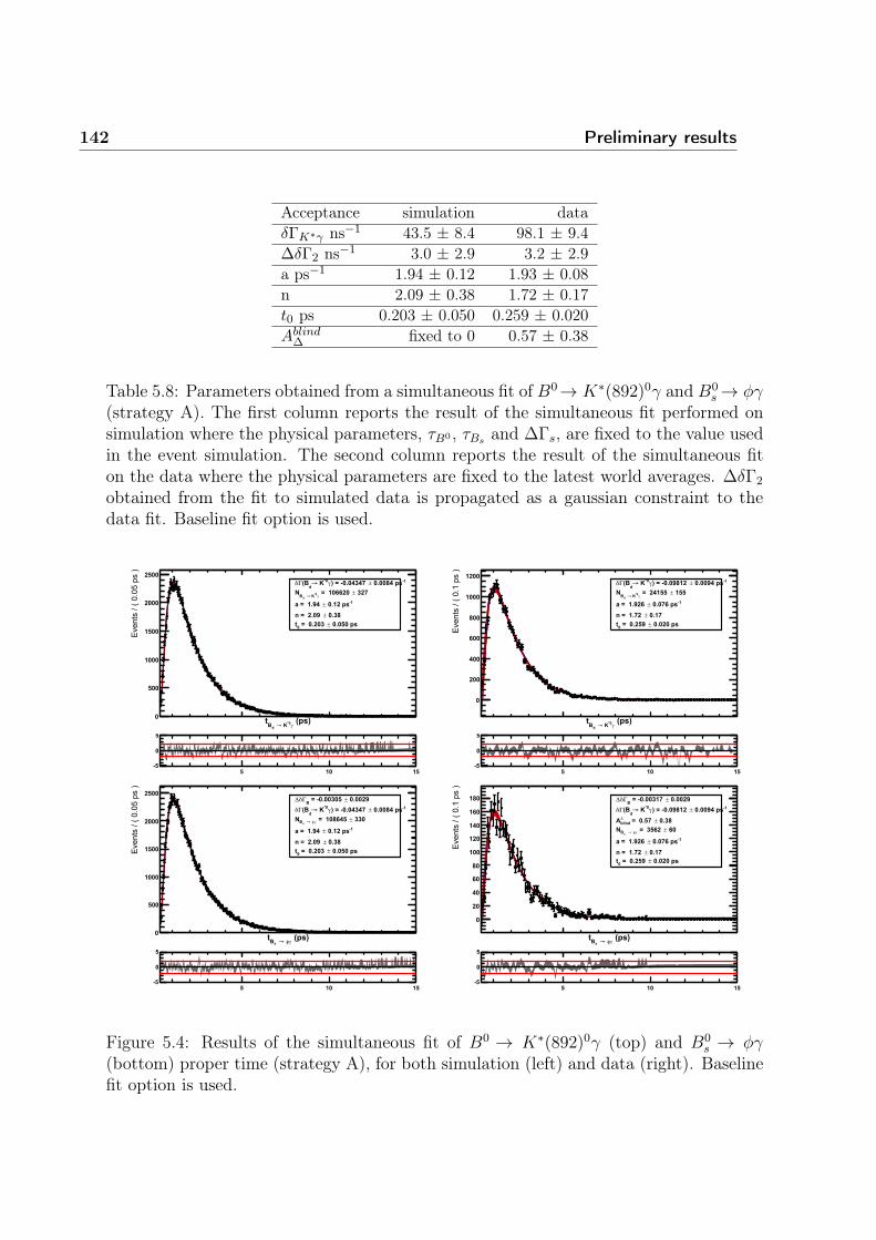
142 Preliminary results
Acceptance simulation dataδΓK∗γ ns−1 43.5 ± 8.4 98.1 ± 9.4ΔδΓ2 ns−1 3.0 ± 2.9 3.2 ± 2.9a ps−1 1.94 ± 0.12 1.93 ± 0.08n 2.09 ± 0.38 1.72 ± 0.17t0 ps 0.203 ± 0.050 0.259 ± 0.020Ablind
Δ fixed to 0 0.57 ± 0.38
Table 5.8: Parameters obtained from a simultaneous fit of B0→ K∗(892)0γ and B0s → φγ
(strategy A). The first column reports the result of the simultaneous fit performed onsimulation where the physical parameters, τB0 , τBs and ΔΓs, are fixed to the value usedin the event simulation. The second column reports the result of the simultaneous fiton the data where the physical parameters are fixed to the latest world averages. ΔδΓ2
obtained from the fit to simulated data is propagated as a gaussian constraint to thedata fit. Baseline fit option is used.
�����γ?��@→�'*
�
�����������#'#,�/���
�
���
����
����
����
����%���&�������±��>�%�&��4�5�γ?��@→
'�*Γδ
�4�5±�>���������γ?��@→�'*
�%���&�����±��>���&6��
��&4�±��>���&�6���&������±�>���&��4���
� �� ��%�
�
�
�����γ?��@→�'*
�
�����������#'"�/���
�
���
���
���
���
����
����%���&��6����±��>�%�&�6����γ?��@→
'�*Γδ
����±�>��������γ?��@→�'*
�%���&�5����±��>���&6���
��&�5±��>���&5����&������±�>���&��6���
� �� ��%�
�
�
�����γφ�→��*
�
�����������#'#,�/���
�
���
����
����
����
������&���6±�>�%�&��4���*ΓδΔ
%���&�������±��>�%�&��4�5�γ?��@→'
�*Γδ
�44�±�>���������γφ�→��*�
%���&�����±��>���&6����&4�±��>���&�6���&������±�>���&��4���
� �� ��%�
�
�
�����γφ�→��*
�
�����������#'"�/���
�
��
��
��
��
���
���
���
���
��� ��&���6±�>�%�&��4�5�*ΓδΔ%���&��6����±��>�%�&�6����γ?��@→
'�*Γδ
��&4�±�>���&�5�;���'Δ3
���±�>��4����γφ�→��*�
%���&�5����±��>���&6�����&�5±��>���&5����&������±�>���&��6���
� �� ��%�
�
�
Figure 5.4: Results of the simultaneous fit of B0 → K∗(892)0γ (top) and B0s → φγ
(bottom) proper time (strategy A), for both simulation (left) and data (right). Baselinefit option is used.
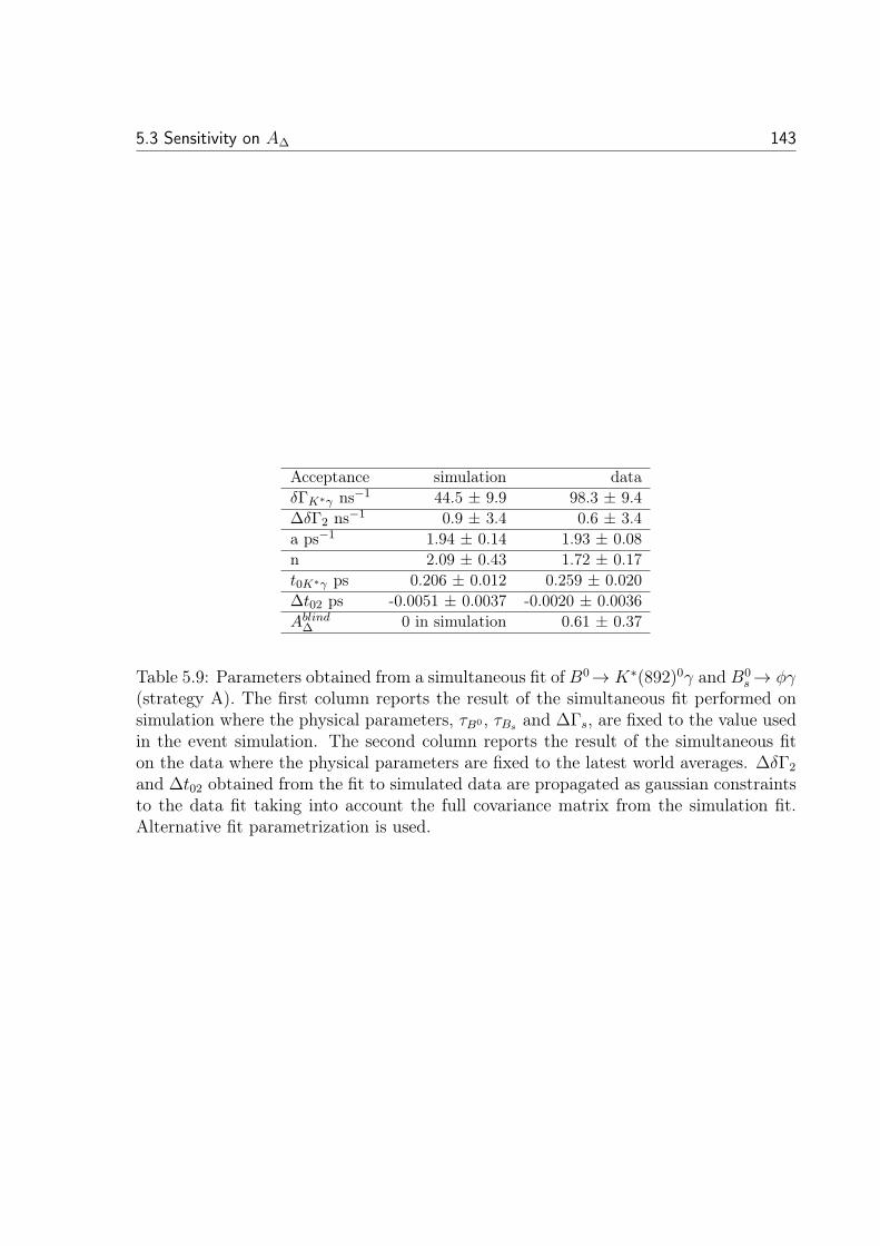
5.3 Sensitivity on AΔ 143
Acceptance simulation dataδΓK∗γ ns−1 44.5 ± 9.9 98.3 ± 9.4ΔδΓ2 ns−1 0.9 ± 3.4 0.6 ± 3.4a ps−1 1.94 ± 0.14 1.93 ± 0.08n 2.09 ± 0.43 1.72 ± 0.17t0K∗γ ps 0.206 ± 0.012 0.259 ± 0.020Δt02 ps -0.0051 ± 0.0037 -0.0020 ± 0.0036Ablind
Δ 0 in simulation 0.61 ± 0.37
Table 5.9: Parameters obtained from a simultaneous fit of B0→ K∗(892)0γ and B0s → φγ
(strategy A). The first column reports the result of the simultaneous fit performed onsimulation where the physical parameters, τB0 , τBs and ΔΓs, are fixed to the value usedin the event simulation. The second column reports the result of the simultaneous fiton the data where the physical parameters are fixed to the latest world averages. ΔδΓ2
and Δt02 obtained from the fit to simulated data are propagated as gaussian constraintsto the data fit taking into account the full covariance matrix from the simulation fit.Alternative fit parametrization is used.
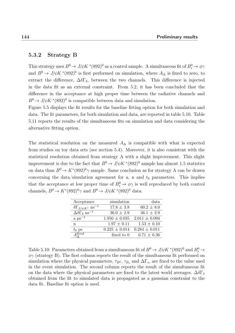
144 Preliminary results
5.3.2 Strategy B
This strategy uses B0→ J/ψK ∗(892)0 as a control sample. A simultaneous fit of B0s → φγ
and B0 → J/ψK ∗(892)0 is first performed on simulation, where AΔ is fixed to zero, toextract the difference, ΔδΓ3, between the two channels. This difference is injectedin the data fit as an external constraint. From 5.2, it has been concluded that thedifference in the acceptance at high proper time between the radiative channels andB0→ J/ψK ∗(892)0 is compatible between data and simulation.Figure 5.5 displays the fit results for the baseline fitting option for both simulation anddata. The fit parameters, for both simulation and data, are reported in table 5.10. Table5.11 reports the results of the simultaneous fits on simulation and data considering thealternative fitting option.
The statistical resolution on the measured AΔ is compatible with what is expectedfrom studies on toy data sets (see section 5.4). Moreover, it is also consistent with thestatistical resolution obtained from strategy A with a slight improvement. This slightimprovement is due to the fact that B0→ J/ψK ∗(892)0 sample has almost 1.5 statisticson data than B0→ K∗(892)0γ sample. Same conclusion as for strategy A can be drawnconcerning the data/simulation agreement for a, n and t0 parameters. This impliesthat the acceptance at low proper time of B0
s → φγ is well reproduced by both controlchannels, B0→ K∗(892)0γ and B0→ J/ψK ∗(892)0 data.
Acceptance simulation dataδΓJ/ψK∗ ns−1 17.8 ± 3.8 60.2 ± 8.0ΔδΓ3 ns−1 36.0 ± 2.9 36.1 ± 2.9a ps−1 1.950 ± 0.035 2.011 ± 0.094n 1.97 ± 0.11 1.53 ± 0.10t0 ps 0.225 ± 0.014 0.284 ± 0.011Ablind
Δ fixed to 0 0.71 ± 0.36
Table 5.10: Parameters obtained from a simultaneous fit of B0→ J/ψK ∗(892)0 and B0s →
φγ (strategy B). The first column reports the result of the simultaneous fit performed onsimulation where the physical parameters, τB0 , τBs and ΔΓs, are fixed to the value usedin the event simulation. The second column reports the result of the simultaneous fiton the data where the physical parameters are fixed to the latest world averages. ΔδΓ3
obtained from the fit to simulated data is propagated as a gaussian constraint to thedata fit. Baseline fit option is used.

5.3 Sensitivity on AΔ 145
�����ψ=)?��@→�'*
�
�����������#'#,�/���
�
���
���
���
���
����
����
����
����
����
����
����
����%���&��4����±��>�%�&��5���ψ=)?��@→
'�*Γδ
�4�6±�>�������6�ψ=)?��@→�'*
�%���&�4����±��>���&6���
��&��±��>���&65���&������±�>���&������
� �� ��%�
�
�
�����ψ=)?��@→�'*
�
�����������#'"�/���
�
���
���
���
���
����
����
����%���&�������±��>�%�&������ψ=)?��@→
'�*Γδ
��5�±�>���6��5�ψ=)?��@→�'*
�%���&�6����±��>���&����
��&��±��>���&�4���&������±�>���&������
� �� ��%�
�
�
�����γφ�→��*
�
�����������#'#,�/���
�
���
����
����
����
������&���6±�>�%�&�4�6��:ΓδΔ
%���&��4����±��>�%�&��5���ψ=)?��@→'
�*Γδ
�44�±�>���������γφ�→��*�
%���&�4����±��>���&6�����&��±��>���&65���&������±�>���&������
� �� ��%�
�
�
�����γφ�→��*
�
�����������#'"�/���
�
��
��
��
��
���
���
���
���
��� ��&���6±�>�%�&�4��5�:ΓδΔ%���&�������±��>�%�&������ψ=)?��@→
'�*Γδ
��&4�±�>���&5��;���'Δ3
���±�>��4����γφ�→��*�
%���&�6����±��>���&������&��±��>���&�4���&������±�>���&������
� �� ��%�
�
�
Figure 5.5: Results of the simultaneous fit of B0 → J/ψK ∗(892)0 (top) and B0s → φγ
(bottom) proper time (strategy B), for both simulation (left) and data (right). Baselinefit option is used.
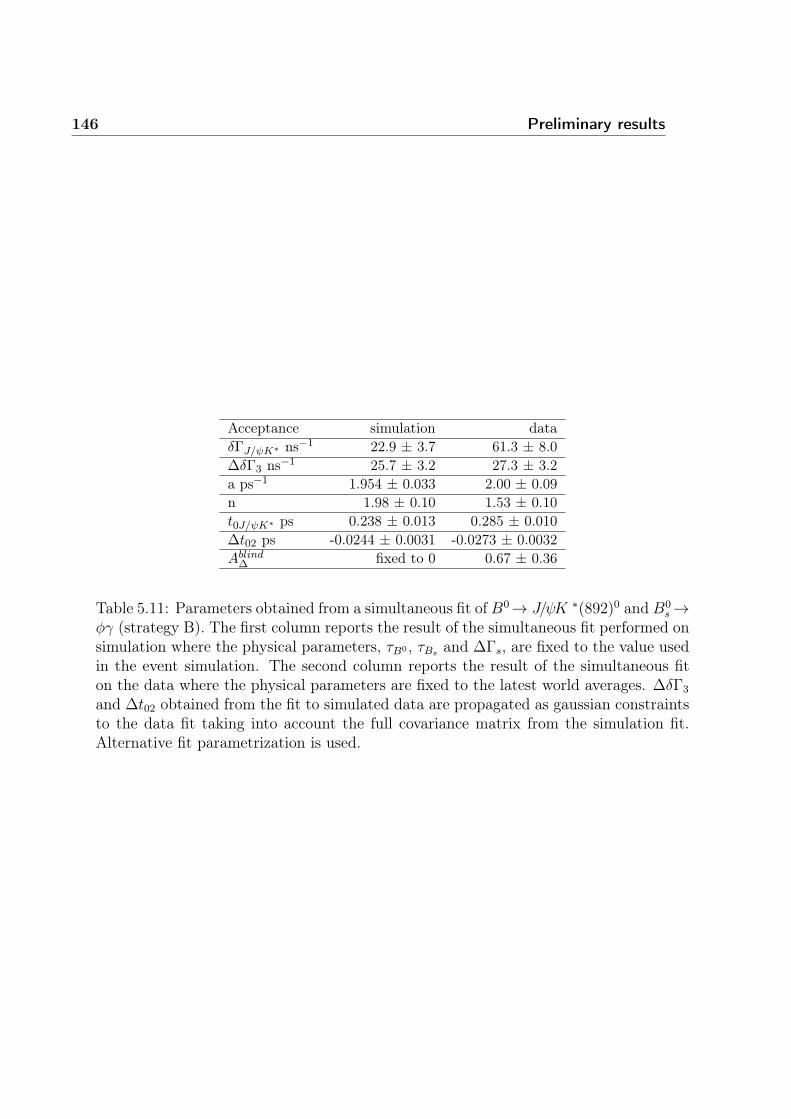
146 Preliminary results
Acceptance simulation dataδΓJ/ψK∗ ns−1 22.9 ± 3.7 61.3 ± 8.0ΔδΓ3 ns−1 25.7 ± 3.2 27.3 ± 3.2a ps−1 1.954 ± 0.033 2.00 ± 0.09n 1.98 ± 0.10 1.53 ± 0.10t0J/ψK∗ ps 0.238 ± 0.013 0.285 ± 0.010Δt02 ps -0.0244 ± 0.0031 -0.0273 ± 0.0032Ablind
Δ fixed to 0 0.67 ± 0.36
Table 5.11: Parameters obtained from a simultaneous fit of B0→ J/ψK ∗(892)0 and B0s →
φγ (strategy B). The first column reports the result of the simultaneous fit performed onsimulation where the physical parameters, τB0 , τBs and ΔΓs, are fixed to the value usedin the event simulation. The second column reports the result of the simultaneous fiton the data where the physical parameters are fixed to the latest world averages. ΔδΓ3
and Δt02 obtained from the fit to simulated data are propagated as gaussian constraintsto the data fit taking into account the full covariance matrix from the simulation fit.Alternative fit parametrization is used.
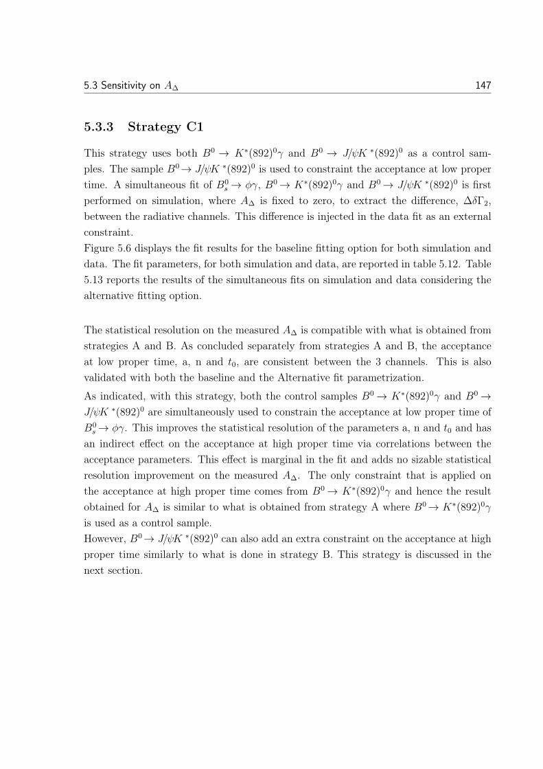
5.3 Sensitivity on AΔ 147
5.3.3 Strategy C1
This strategy uses both B0 → K∗(892)0γ and B0 → J/ψK ∗(892)0 as a control sam-ples. The sample B0→ J/ψK ∗(892)0 is used to constraint the acceptance at low propertime. A simultaneous fit of B0
s → φγ, B0→ K∗(892)0γ and B0→ J/ψK ∗(892)0 is firstperformed on simulation, where AΔ is fixed to zero, to extract the difference, ΔδΓ2,between the radiative channels. This difference is injected in the data fit as an externalconstraint.Figure 5.6 displays the fit results for the baseline fitting option for both simulation anddata. The fit parameters, for both simulation and data, are reported in table 5.12. Table5.13 reports the results of the simultaneous fits on simulation and data considering thealternative fitting option.
The statistical resolution on the measured AΔ is compatible with what is obtained fromstrategies A and B. As concluded separately from strategies A and B, the acceptanceat low proper time, a, n and t0, are consistent between the 3 channels. This is alsovalidated with both the baseline and the Alternative fit parametrization.
As indicated, with this strategy, both the control samples B0 → K∗(892)0γ and B0 →J/ψK ∗(892)0 are simultaneously used to constrain the acceptance at low proper time ofB0
s → φγ. This improves the statistical resolution of the parameters a, n and t0 and hasan indirect effect on the acceptance at high proper time via correlations between theacceptance parameters. This effect is marginal in the fit and adds no sizable statisticalresolution improvement on the measured AΔ. The only constraint that is applied onthe acceptance at high proper time comes from B0 → K∗(892)0γ and hence the resultobtained for AΔ is similar to what is obtained from strategy A where B0→ K∗(892)0γ
is used as a control sample.However, B0→ J/ψK ∗(892)0 can also add an extra constraint on the acceptance at highproper time similarly to what is done in strategy B. This strategy is discussed in thenext section.
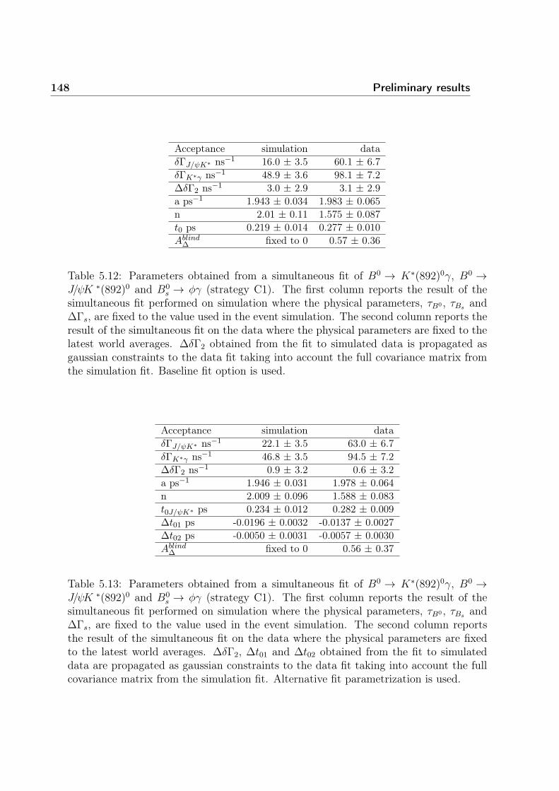
148 Preliminary results
Acceptance simulation dataδΓJ/ψK∗ ns−1 16.0 ± 3.5 60.1 ± 6.7δΓK∗γ ns−1 48.9 ± 3.6 98.1 ± 7.2ΔδΓ2 ns−1 3.0 ± 2.9 3.1 ± 2.9a ps−1 1.943 ± 0.034 1.983 ± 0.065n 2.01 ± 0.11 1.575 ± 0.087t0 ps 0.219 ± 0.014 0.277 ± 0.010Ablind
Δ fixed to 0 0.57 ± 0.36
Table 5.12: Parameters obtained from a simultaneous fit of B0 → K∗(892)0γ, B0 →J/ψK ∗(892)0 and B0
s → φγ (strategy C1). The first column reports the result of thesimultaneous fit performed on simulation where the physical parameters, τB0 , τBs andΔΓs, are fixed to the value used in the event simulation. The second column reports theresult of the simultaneous fit on the data where the physical parameters are fixed to thelatest world averages. ΔδΓ2 obtained from the fit to simulated data is propagated asgaussian constraints to the data fit taking into account the full covariance matrix fromthe simulation fit. Baseline fit option is used.
Acceptance simulation dataδΓJ/ψK∗ ns−1 22.1 ± 3.5 63.0 ± 6.7δΓK∗γ ns−1 46.8 ± 3.5 94.5 ± 7.2ΔδΓ2 ns−1 0.9 ± 3.2 0.6 ± 3.2a ps−1 1.946 ± 0.031 1.978 ± 0.064n 2.009 ± 0.096 1.588 ± 0.083t0J/ψK∗ ps 0.234 ± 0.012 0.282 ± 0.009Δt01 ps -0.0196 ± 0.0032 -0.0137 ± 0.0027Δt02 ps -0.0050 ± 0.0031 -0.0057 ± 0.0030Ablind
Δ fixed to 0 0.56 ± 0.37
Table 5.13: Parameters obtained from a simultaneous fit of B0 → K∗(892)0γ, B0 →J/ψK ∗(892)0 and B0
s → φγ (strategy C1). The first column reports the result of thesimultaneous fit performed on simulation where the physical parameters, τB0 , τBs andΔΓs, are fixed to the value used in the event simulation. The second column reportsthe result of the simultaneous fit on the data where the physical parameters are fixedto the latest world averages. ΔδΓ2, Δt01 and Δt02 obtained from the fit to simulateddata are propagated as gaussian constraints to the data fit taking into account the fullcovariance matrix from the simulation fit. Alternative fit parametrization is used.
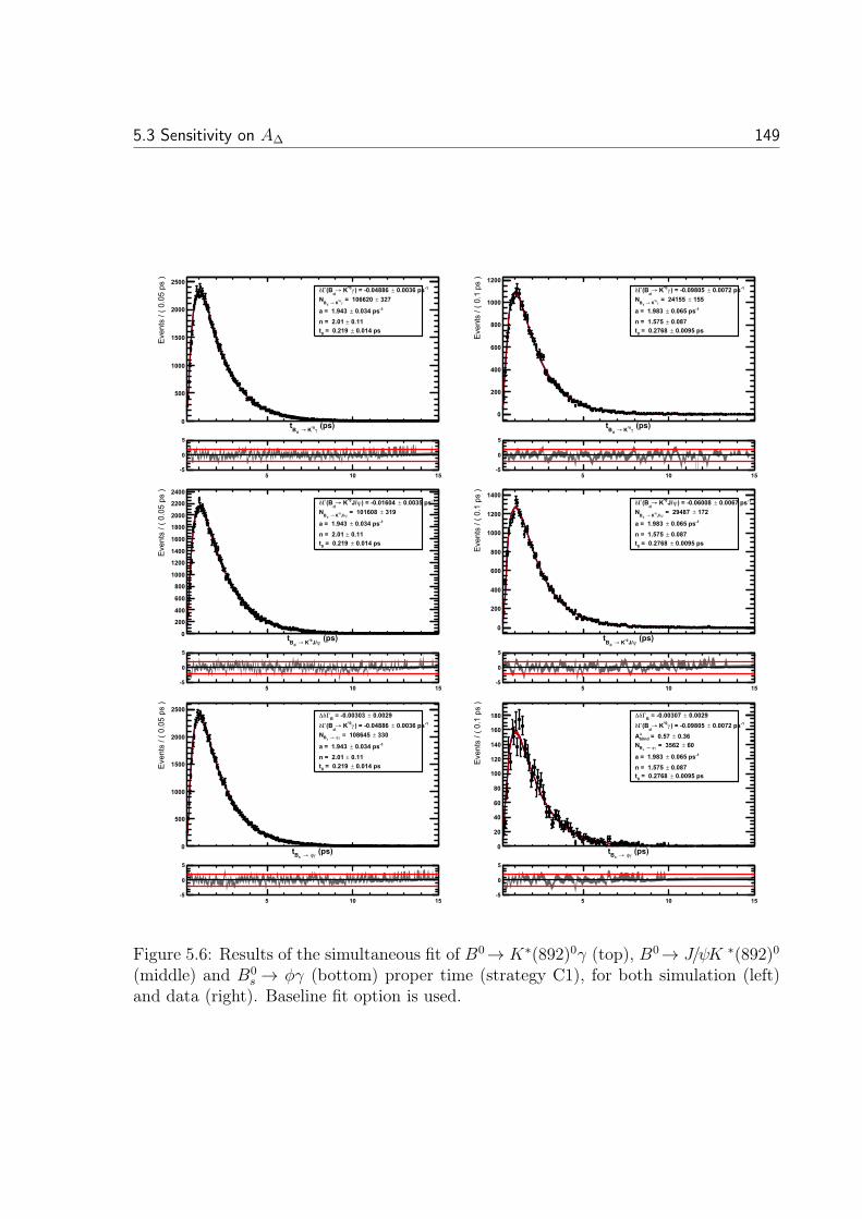
5.3 Sensitivity on AΔ 149
�����γ?��@→�'*
�
�����������#'#,�/���
�
���
����
����
����
����%���&��4����±��>�%�&������γ?��@→
'�*Γδ
�4�5±�>���������γ?��@→�'*
�%���&�4����±��>���&6�4�
��&��±��>���&�����&������±�>���&��6���
� �� ��%�
�
�
�����γ?��@→�'*
�
�����������#'"�/���
�
���
���
���
���
����
����%���&��5����±��>�%�&�6����γ?��@→
'�*Γδ
����±�>��������γ?��@→�'*
�%���&������±��>���&6�4�
��&��5±��>���&�5����&��6����±�>���&�5�����
� �� ��%�
�
�
�����ψ=)?��@→�'*
�
�����������#'#,�/���
�
���
���
���
���
����
����
����
����
����
����
����
����%���&��4����±��>�%�&������ψ=)?��@→
'�*Γδ
�4�6±�>���������ψ=)?��@→�'*
�%���&�4����±��>���&6�4�
��&��±��>���&�����&������±�>���&��6���
� �� ��%�
�
�
�����ψ=)?��@→�'*
�
�����������#'"�/���
�
���
���
���
���
����
����
����%���&���5���±��>�%�&������ψ=)?��@→
'�*Γδ
��5�±�>���6��5�ψ=)?��@→�'*
�%���&������±��>���&6�4�
��&��5±��>���&�5����&��6����±�>���&�5�����
� �� ��%�
�
�
�����γφ�→��*
�
�����������#'#,�/���
�
���
����
����
����
������&���6±�>�%�&��4�4�*ΓδΔ
%���&��4����±��>�%�&������γ?��@→'
�*Γδ
�44�±�>���������γφ�→��*�
%���&�4����±��>���&6�4���&��±��>���&�����&������±�>���&��6���
� �� ��%�
�
�
�����γφ�→��*
�
�����������#'"�/���
�
��
��
��
��
���
���
���
���
��� ��&���6±�>�%�&��4�5�*ΓδΔ%���&��5����±��>�%�&�6����γ?��@→
'�*Γδ
��&4�±�>���&�5�;���'Δ3
���±�>��4����γφ�→��*�
%���&������±��>���&6�4���&��5±��>���&�5����&��6����±�>���&�5�����
� �� ��%�
�
�
Figure 5.6: Results of the simultaneous fit of B0→ K∗(892)0γ (top), B0→ J/ψK ∗(892)0
(middle) and B0s → φγ (bottom) proper time (strategy C1), for both simulation (left)
and data (right). Baseline fit option is used.
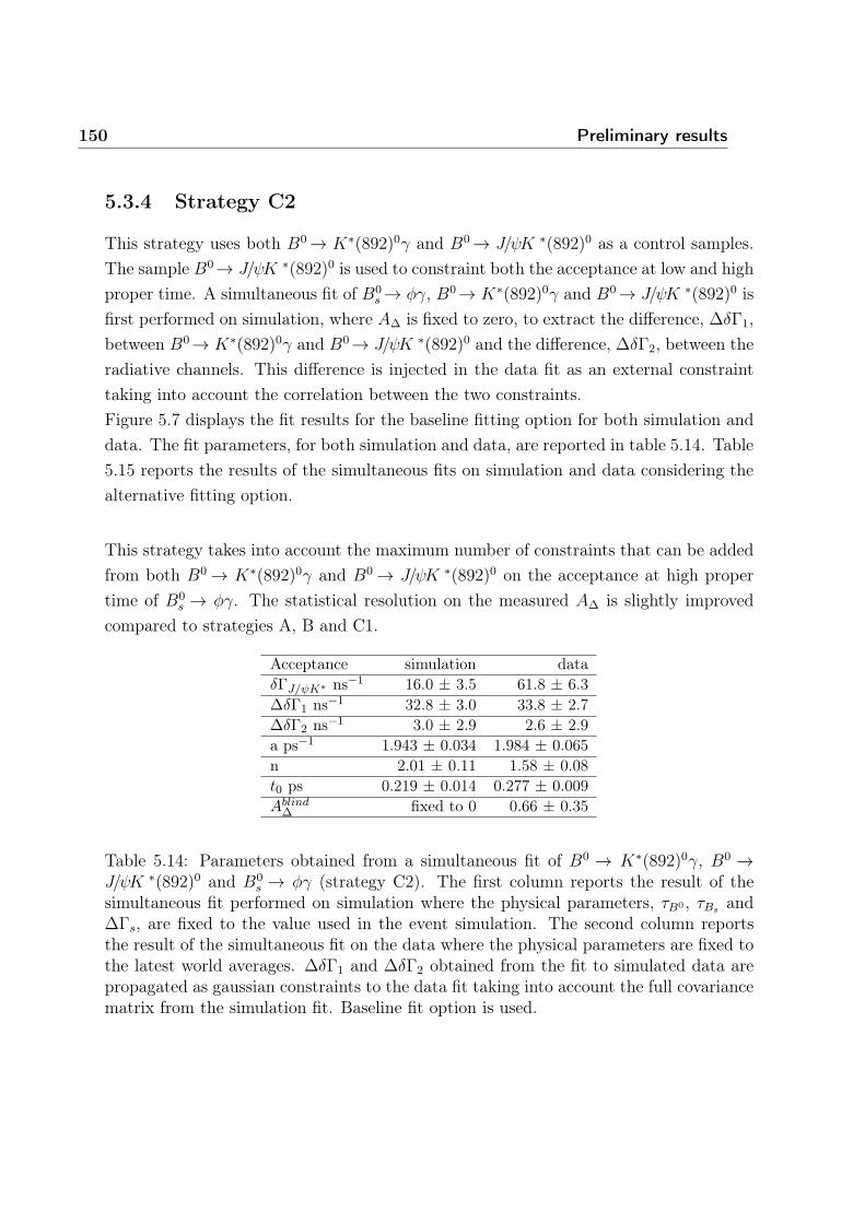
150 Preliminary results
5.3.4 Strategy C2
This strategy uses both B0→ K∗(892)0γ and B0→ J/ψK ∗(892)0 as a control samples.The sample B0→ J/ψK ∗(892)0 is used to constraint both the acceptance at low and highproper time. A simultaneous fit of B0
s → φγ, B0→ K∗(892)0γ and B0→ J/ψK ∗(892)0 isfirst performed on simulation, where AΔ is fixed to zero, to extract the difference, ΔδΓ1,between B0→ K∗(892)0γ and B0→ J/ψK ∗(892)0 and the difference, ΔδΓ2, between theradiative channels. This difference is injected in the data fit as an external constrainttaking into account the correlation between the two constraints.Figure 5.7 displays the fit results for the baseline fitting option for both simulation anddata. The fit parameters, for both simulation and data, are reported in table 5.14. Table5.15 reports the results of the simultaneous fits on simulation and data considering thealternative fitting option.
This strategy takes into account the maximum number of constraints that can be addedfrom both B0 → K∗(892)0γ and B0 → J/ψK ∗(892)0 on the acceptance at high propertime of B0
s → φγ. The statistical resolution on the measured AΔ is slightly improvedcompared to strategies A, B and C1.
Acceptance simulation dataδΓJ/ψK∗ ns−1 16.0 ± 3.5 61.8 ± 6.3ΔδΓ1 ns−1 32.8 ± 3.0 33.8 ± 2.7ΔδΓ2 ns−1 3.0 ± 2.9 2.6 ± 2.9a ps−1 1.943 ± 0.034 1.984 ± 0.065n 2.01 ± 0.11 1.58 ± 0.08t0 ps 0.219 ± 0.014 0.277 ± 0.009Ablind
Δ fixed to 0 0.66 ± 0.35
Table 5.14: Parameters obtained from a simultaneous fit of B0 → K∗(892)0γ, B0 →J/ψK ∗(892)0 and B0
s → φγ (strategy C2). The first column reports the result of thesimultaneous fit performed on simulation where the physical parameters, τB0 , τBs andΔΓs, are fixed to the value used in the event simulation. The second column reportsthe result of the simultaneous fit on the data where the physical parameters are fixed tothe latest world averages. ΔδΓ1 and ΔδΓ2 obtained from the fit to simulated data arepropagated as gaussian constraints to the data fit taking into account the full covariancematrix from the simulation fit. Baseline fit option is used.
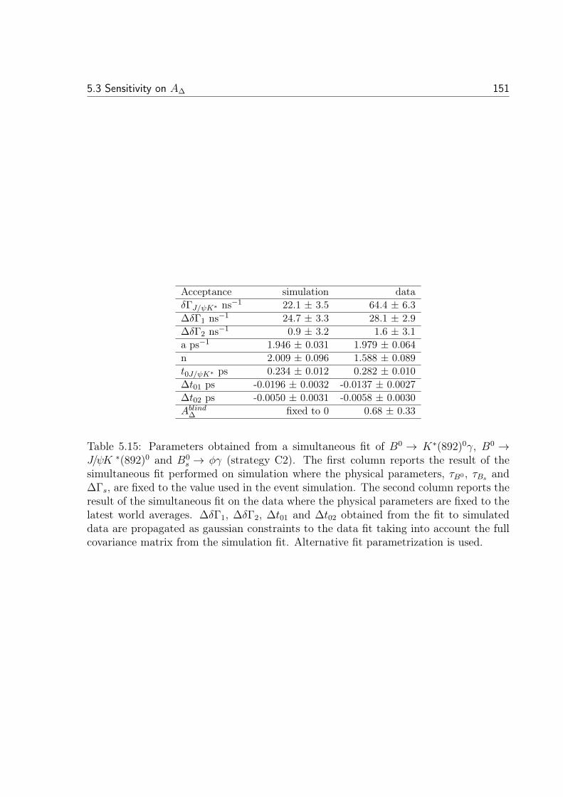
5.3 Sensitivity on AΔ 151
Acceptance simulation dataδΓJ/ψK∗ ns−1 22.1 ± 3.5 64.4 ± 6.3ΔδΓ1 ns−1 24.7 ± 3.3 28.1 ± 2.9ΔδΓ2 ns−1 0.9 ± 3.2 1.6 ± 3.1a ps−1 1.946 ± 0.031 1.979 ± 0.064n 2.009 ± 0.096 1.588 ± 0.089t0J/ψK∗ ps 0.234 ± 0.012 0.282 ± 0.010Δt01 ps -0.0196 ± 0.0032 -0.0137 ± 0.0027Δt02 ps -0.0050 ± 0.0031 -0.0058 ± 0.0030Ablind
Δ fixed to 0 0.68 ± 0.33
Table 5.15: Parameters obtained from a simultaneous fit of B0 → K∗(892)0γ, B0 →J/ψK ∗(892)0 and B0
s → φγ (strategy C2). The first column reports the result of thesimultaneous fit performed on simulation where the physical parameters, τB0 , τBs andΔΓs, are fixed to the value used in the event simulation. The second column reports theresult of the simultaneous fit on the data where the physical parameters are fixed to thelatest world averages. ΔδΓ1, ΔδΓ2, Δt01 and Δt02 obtained from the fit to simulateddata are propagated as gaussian constraints to the data fit taking into account the fullcovariance matrix from the simulation fit. Alternative fit parametrization is used.
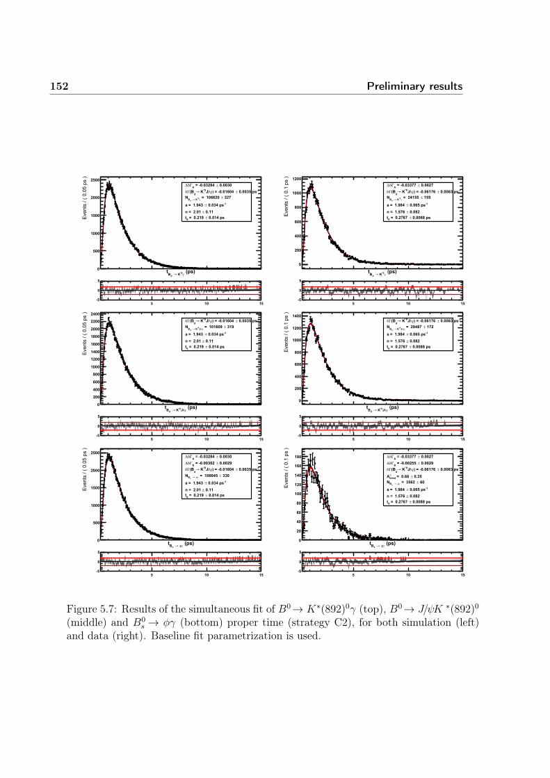
152 Preliminary results
�����γ?��@→�'*
�
�����������#'#,�/���
�
���
����
����
����
������&��4�±�>�%�&�4����3ΓδΔ
%���&��4����±��>�%�&������ψ=)?��@→'
�*Γδ
�4�5±�>���������γ?��@→�'*
�%���&�4����±��>���&6�4�
��&��±��>���&�����&������±�>���&��6���
� �� ��%�
�
�
�����γ?��@→�'*
�
�����������#'"�/���
�
���
���
���
���
����
������&���5±�>�%�&�4455�3ΓδΔ
%���&���4���±��>�%�&���5��ψ=)?��@→'
�*Γδ
����±�>��������γ?��@→�'*
�%���&������±��>���&6���
��&���±��>���&�5����&�������±�>���&�5�5���
� �� ��%�
�
�
�����ψ=)?��@→�'*
�
�����������#'#,�/���
�
���
���
���
���
����
����
����
����
����
����
����
����%���&��4����±��>�%�&������ψ=)?��@→
'�*Γδ
�4�6±�>�������6�ψ=)?��@→�'*
�%���&�4����±��>���&6�4�
��&��±��>���&�����&������±�>���&��6���
� �� ��%�
�
�
�����ψ=)?��@→�'*
�
�����������#'"�/���
�
���
���
���
���
����
����
����%���&���4���±��>�%�&���5��ψ=)?��@→
'�*Γδ
��5�±�>���6��5�ψ=)?��@→�'*
�%���&������±��>���&6���
��&���±��>���&�5����&�������±�>���&�5�5���
� �� ��%�
�
�
�����γφ�→��*
�
�����������#'#,�/���
�
���
����
����
����
������&��4�±�>�%�&�4����3ΓδΔ
��&���6±�>�%�&��4���*ΓδΔ%���&��4����±��>�%�&������ψ=)?��@→
'�*Γδ
�44�±�>���������γφ�→��*�
%���&�4����±��>���&6�4���&��±��>���&�����&������±�>���&��6���
� �� ��%�
�
�
�����γφ�→��*
�
�����������#'"�/���
�
��
��
��
��
���
���
���
���
��� ��&���5±�>�%�&�4455�3ΓδΔ
��&���6±�>�%�&������*ΓδΔ%���&���4���±��>�%�&���5��ψ=)?��@→
'�*Γδ
��&4�±�>���&���;���'Δ3
���±�>��4����γφ�→��*�
%���&������±��>���&6�����&���±��>���&�5����&�������±�>���&�5�5���
� �� ��%�
�
�
Figure 5.7: Results of the simultaneous fit of B0→ K∗(892)0γ (top), B0→ J/ψK ∗(892)0
(middle) and B0s → φγ (bottom) proper time (strategy C2), for both simulation (left)
and data (right). Baseline fit parametrization is used.
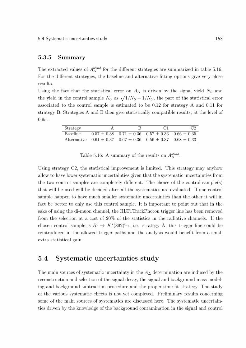
5.4 Systematic uncertainties study 153
5.3.5 Summary
The extracted values of AblindΔ for the different strategies are summarized in table 5.16.
For the different strategies, the baseline and alternative fitting options give very closeresults.Using the fact that the statistical error on AΔ is driven by the signal yield NS andthe yield in the control sample NC as
√1/NS + 1/NC , the part of the statistical error
associated to the control sample is estimated to be 0.12 for strategy A and 0.11 forstrategy B. Strategies A and B then give statistically compatible results, at the level of0.9σ.
Strategy A B C1 C2Baseline 0.57 ± 0.38 0.71 ± 0.36 0.57 ± 0.36 0.66 ± 0.35Alternative 0.61 ± 0.37 0.67 ± 0.36 0.56 ± 0.37 0.68 ± 0.33
Table 5.16: A summary of the results on AblindΔ .
Using strategy C2, the statistical improvement is limited. This strategy may anyhowallow to have lower systematic uncertainties given that the systematic uncertainties fromthe two control samples are completely different. The choice of the control sample(s)that will be used will be decided after all the systematics are evaluated. If one controlsample happen to have much smaller systematic uncertainties than the other it will infact be better to only use this control sample. It is important to point out that in thesake of using the di-muon channel, the HLT1TrackPhoton trigger line has been removedfrom the selection at a cost of 20% of the statistics in the radiative channels. If thechosen control sample is B0 → K∗(892)0γ, i.e. strategy A, this trigger line could bereintroduced in the allowed trigger paths and the analysis would benefit from a smallextra statistical gain.
5.4 Systematic uncertainties study
The main sources of systematic uncertainty in the AΔ determination are induced by thereconstruction and selection of the signal decay, the signal and background mass model-ing and background subtraction procedure and the proper time fit strategy. The studyof the various systematic effects is not yet completed. Preliminary results concerningsome of the main sources of systematics are discussed here. The systematic uncertain-ties driven by the knowledge of the background contamination in the signal and control
154 Preliminary results
samples and its subtraction procedure is discussed in 5.4.1 where a brief summary of thework performed by our collaborators in the EPFL Lausanne group is presented. The un-certainty due to the limited knowledge of the external physical parameters is addressedin 5.4.2. The impact of the scaling and weighing procedures is discussed in 5.4.3. Othersystematics that are still under study are discussed in section 5.4.4.
5.4.1 Background contamination and modeling
The AΔ extraction relies on the good control of the background subtraction procedure.For instance imperfections in the modeling of the reconstructed mass shape would alterthe background-subtracted proper time distribution and thus affect the AΔ determina-tion. Moreover, the expected small contamination of the backgrounds peaking in thesignal mass region is not subtracted in the procedure as explained in section 4.2.3.Some of the systematic uncertainties due to the reliability of the background subtractioncan be investigated by a toys procedure approach. This procedure consists in generatinga large amount of simulated data sets using a defined fit model with varying the inputparameters in the range of their error. These data sets are fitted with the same modelletting free the parameters so as to test the bias that the used model introduce on themeasured parameters. Moreover, simulated data sets can be generated assuming a givenhypotheses for a model, and then fitted assuming a different hypotheses so as to studythe effect of this given hypotheses on the measured value of the model’s parameters.Several systematic effects related to the level of background contamination have beenstudied this way and are discussed in the following. The impact on the measurementinduced by an imperfect mass modeling is not fully addressed by those tests. Additionalsystematic uncertainties can be estimated by repeating the full analysis varying the massshape description for the various contributions to the selected sample.
The validity of the fit model has been studied using the toy procedure. The study con-sists in generating the mass distribution with all the physical backgrounds, taking intoaccount the number of events extracted from the fit to data. This mass distribution isthen background subtracted and fitted following the procedure describe in 4.2.3. Forradiative decays, background is subtracted using the sPlot technique where the back-ground contamination peaking in the signal region are considered as part of signal. ForB0→ J/ψK ∗(892)0, signal data is selected by cutting around the mass peak. The simul-taneous fits from strategies A, B and C2 are then performed on the signal proper time

5.4 Systematic uncertainties study 155
μ(AΔFIT − AΔINPUT) σ(AΔFIT)Strategy A 0.022±0.007 0.338±0.005Strategy B 0.063±0.005 0.308±0.003Strategy C2 0.022±0.007 0.307±0.006
Table 5.17: Average central value and resolution for AΔ obtained from 1000 toys con-sidering the mass and proper time fitting models.
distribution using the procedure described in 5.3 The average central value and resolu-tion for the AΔ parameters obtained from a large set of toys are reported in table 5.17.The average statistical resolution on AΔ, of the order of 0.34 for strategy A and 0.31for strategy B and C2, is compatible with what is measured on data. It can be noticedthat the average expected resolution is slightly improved with strategy C2 compared tostrategy A.A bias on the central value of the order of 0.02 for strategy A and C2 and of the order of0.06 for strategy B is observed. This bias is induced by the treatment of the backgroundpeaking in the signal mass region as explained in the following.Figure 5.8 displays the pull distribution of the toy sample for the parameter AΔ, definedas :
AΔFIT − AΔINPUT
σ(AΔFIT),
for strategies A, B and C2. The small bias on the AΔ determination is quantified bythe parameters of the gaussian fit of the pull distribution which are expected to be (μ,σ)=(0, 1) for an unbiased distribution in the limit of an infinite size sample.
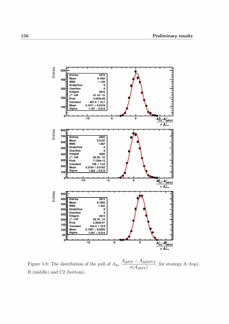
156 Preliminary results
Figure 5.8: The distribution of the pull of AΔ,AΔFIT − AΔINPUT
σ(AΔFIT), for strategy A (top),
B (middle) and C2 (bottom).
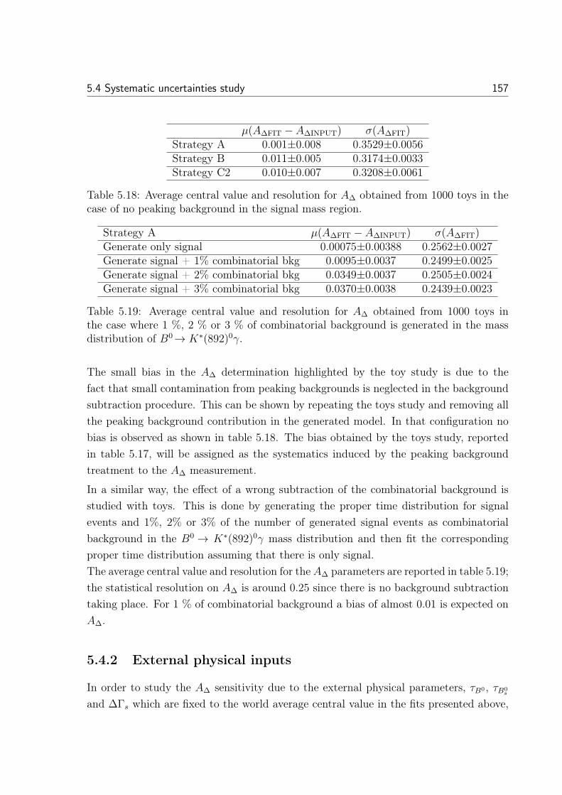
5.4 Systematic uncertainties study 157
μ(AΔFIT − AΔINPUT) σ(AΔFIT)Strategy A 0.001±0.008 0.3529±0.0056Strategy B 0.011±0.005 0.3174±0.0033Strategy C2 0.010±0.007 0.3208±0.0061
Table 5.18: Average central value and resolution for AΔ obtained from 1000 toys in thecase of no peaking background in the signal mass region.
Strategy A μ(AΔFIT − AΔINPUT) σ(AΔFIT)Generate only signal 0.00075±0.00388 0.2562±0.0027Generate signal + 1% combinatorial bkg 0.0095±0.0037 0.2499±0.0025Generate signal + 2% combinatorial bkg 0.0349±0.0037 0.2505±0.0024Generate signal + 3% combinatorial bkg 0.0370±0.0038 0.2439±0.0023
Table 5.19: Average central value and resolution for AΔ obtained from 1000 toys inthe case where 1 %, 2 % or 3 % of combinatorial background is generated in the massdistribution of B0→ K∗(892)0γ.
The small bias in the AΔ determination highlighted by the toy study is due to thefact that small contamination from peaking backgrounds is neglected in the backgroundsubtraction procedure. This can be shown by repeating the toys study and removing allthe peaking background contribution in the generated model. In that configuration nobias is observed as shown in table 5.18. The bias obtained by the toys study, reportedin table 5.17, will be assigned as the systematics induced by the peaking backgroundtreatment to the AΔ measurement.
In a similar way, the effect of a wrong subtraction of the combinatorial background isstudied with toys. This is done by generating the proper time distribution for signalevents and 1%, 2% or 3% of the number of generated signal events as combinatorialbackground in the B0 → K∗(892)0γ mass distribution and then fit the correspondingproper time distribution assuming that there is only signal.The average central value and resolution for the AΔ parameters are reported in table 5.19;the statistical resolution on AΔ is around 0.25 since there is no background subtractiontaking place. For 1 % of combinatorial background a bias of almost 0.01 is expected onAΔ.
5.4.2 External physical inputs
In order to study the AΔ sensitivity due to the external physical parameters, τB0 , τB0s
and ΔΓs which are fixed to the world average central value in the fits presented above,
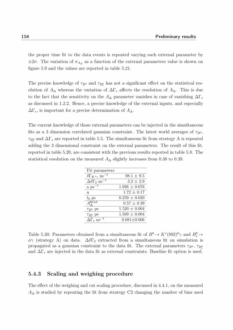
158 Preliminary results
the proper time fit to the data events is repeated varying each external parameter by±2σ. The variation of σAΔ
as a function of the external parameters value is shown onfigure 5.9 and the values are reported in table 5.21.
The precise knowledge of τB0 and τB0s
has not a significant effect on the statistical res-olution of AΔ whereas the variation of ΔΓs affects the resolution of AΔ. This is dueto the fact that the sensitivity on the AΔ parameter vanishes in case of vanishing ΔΓs
as discussed in 1.2.2. Hence, a precise knowledge of the external inputs, and especiallyΔΓs, is important for a precise determination of AΔ.
The current knowledge of those external parameters can be injected in the simultaneousfits as a 3 dimension correlated gaussian constraint. The latest world averages of τB0 ,τB0
sand ΔΓs are reported in table 5.5. The simultaneous fit from strategy A is repeated
adding the 3 dimensional constraint on the external parameters. The result of this fit,reported in table 5.20, are consistent with the previous results reported in table 5.8. Thestatistical resolution on the measured AΔ slightly increases from 0.38 to 0.39.
Fit parametersδΓK∗γ ns−1 98.1 ± 9.5ΔδΓ2 ns−1 3.2 ± 2.9a ps−1 1.926 ± 0.076n 1.72 ± 0.17t0 ps 0.259 ± 0.020Ablind
Δ 0.57 ± 0.39τB0 ps 1.520 ± 0.004τB0
sps 1.509 ± 0.004
ΔΓs ns−1 0.081±0.006
Table 5.20: Parameters obtained from a simultaneous fit of B0→ K∗(892)0γ and B0s →
φγ (strategy A) on data. ΔδΓ2 extracted from a simultaneous fit on simulation ispropagated as a gaussian constraint to the data fit. The external parameters τB0 , τB0
s
and ΔΓs are injected in the data fit as external constraints. Baseline fit option is used.
5.4.3 Scaling and weighing procedure
The effect of the weighing and cut scaling procedure, discussed in 4.4.1, on the measuredAΔ is studied by repeating the fit from strategy C2 changing the number of bins used
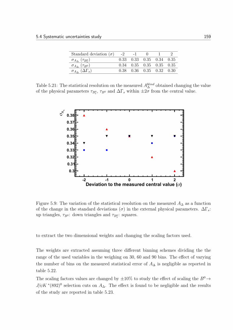
5.4 Systematic uncertainties study 159
Standard deviation (σ) -2 -1 0 1 2σAΔ
(τB0s) 0.33 0.33 0.35 0.34 0.35
σAΔ(τB0) 0.34 0.35 0.35 0.35 0.35
σAΔ(ΔΓs) 0.38 0.36 0.35 0.32 0.30
Table 5.21: The statistical resolution on the measured AblindΔ obtained changing the value
of the physical parameters τB0s, τB0 and ΔΓs within ±2σ from the central value.
��σ��8��������������<���,$�'�����$���8��,���%� %� � � �
Δ4σ
�&4
�&4�
�&4�
�&44
�&4�
�&4�
�&4�
�&45
�&4�
Figure 5.9: The variation of the statistical resolution on the measured AΔ as a functionof the change in the standard deviations (σ) in the external physical parameters. ΔΓs:up triangles, τB0 : down triangles and τB0
s: squares.
to extract the two dimensional weights and changing the scaling factors used.
The weights are extracted assuming three different binning schemes dividing the therange of the used variables in the weighing on 30, 60 and 90 bins. The effect of varyingthe number of bins on the measured statistical error of AΔ is negligible as reported intable 5.22.
The scaling factors values are changed by ±10% to study the effect of scaling the B0→J/ψK ∗(892)0 selection cuts on AΔ. The effect is found to be negligible and the resultsof the study are reported in table 5.23.

160 Preliminary results
Number of bins 30 60 90σAΔ
0.35 0.34 0.35
Table 5.22: The statistical resolution on the measured AblindΔ extracted changing the
number of bins used to obtain two dimensional weights of B0 → J/ψK ∗(892)0. Theeventual change in the central value is to be taken as a systematic. Strategy C1 is used.
Scaling factor deviation -10% 0% +10%σAΔ
(changing θDIRA) 0.35 0.35 0.34σAΔ
(changing χ2(IPK+)) 0.34 0.35 0.35σAΔ
(changing χ2(IPπ−)) 0.33 0.35 0.34
Table 5.23: The statistical resolution on the measured AblindΔ extracted changing the
scaling factors by ±10%. The eventual change in the central value is to be taken as asystematic. Strategy C1 is used.
5.4.4 Other systematics
Many other possible systematics effects are being investigated:
• The effect on AΔ due to fixing the shapes of the different contributions to the massmodel for B0→ K∗(892)0γ and B0
s → φγ from simulation.
• The effect on AΔ due to the photon calibration, discussed in appendix B, can bestudied by varying the photon energy in B0→ K∗(892)0γ and B0
s → φγ.
• The effect of assuming the parameters of the acceptance at low proper time to becommon for the signal and control sample(s), mainly parameters a and n, can bestudied by performing a fit where a and n are assumed to not be common for thechannels, as done for t0 in the alternative fit, and add a constraint, extracted fromthe fit to simulated events, on the difference Δa and Δn in the data fit.
• The effect of changing the analytical parametrization of the proper time acceptanceon the measured AΔ can be studied by choosing a different acceptance functionand redoing the proper time fits.
• The effect of the possible correlations between mass and proper time can be studiedby toys similar to the full toy study except that simulation events are used for thesignal and for the control samples.
5.5 Conclusions 161
• The time-dependent decay rate for the untagged B0s → φγ decay given in equa-
tion 4.4 and used in the proper time fit model relies on the cancellation of theflavor dependent oscillation terms. Due to a possible small flavor asymmetry inBs production at LHC, measured to be AP (Bs) = (1.09± 2.61± 0.66)% [109], thecancellation might not realize perfectly and the systematic effect has to be prop-agated on the AΔ determination. The related uncertainty is however expectedto be negligible thanks to the small measured Bs production asymmetry and theexpected small CCP and SCP terms.
5.5 Conclusions
In this work, four different strategies to measure AΔ have been studied. The differentstrategies give statistically compatible results for AΔ. The expected statistical uncer-tainty on the measured AΔ is of about 0.35. This is compatible with the expectedresolution obtained from the study based on a large toys sample. Strategy C2, whereboth B0→ K∗(892)0γ and B0→ J/ψK ∗(892)0 are used as control samples, has a slightlybetter statistical resolution on AΔ.
The baseline fit option has shown that there is a good control of the acceptance at lowproper time. This is validated by an alternative fit parametrization where one of theparameters modeling the acceptance at low proper time is considered to not be the samefor the different channels in the simultaneous fit. Both the baseline fit and the alterna-tive fit give compatible results.
The analysis is in the finalization phase with the following steps to be completed beforeperforming a final unblinded measurement:
• Some of the systematic uncertainties are studied, mainly the systematic due tothe mis-knowledge of the level of contamination of the different backgrounds, theeffect due to the external physical parameters and the effect of the weighing andcut scaling procedure performed to align the acceptance of B0 → J/ψK ∗(892)0
with B0→ K∗(892)0γ. Other systematic effects are under study.
• The difference in the acceptance at high proper time between data and simulationremains to be understood.

162 Preliminary results
• The performance of the AΔ extraction is to be compared with the proper time ratiofit approach developed by our collaborators from Valencia. Preliminary comparisonshows a similar statistical sensitivity for both extraction methods. The comparedsensitivity to systematical effects is under investigation.
Conclusion
B physics is an important field of research providing a concret testing ground ofthe Standard Model (SM) on the experimental and the theoretical sides. In this context,studying the radiative decays of the B meson stands as a probe of New Physics (NP)phenomena. The measurement of the photon polarization in b → sγ radiative penguintransition can put some constraints on NP scenarios.
With the data collected during its first phase of operation, LHCb has already demon-strated its capability to reconstruct radiative decays, many of which have already beenanalyzed and studied. The first measurement of the photon polarization is addressed inseveral analysis at LHCb. An angular analysis of B → K∗e+e− is performed to measurethe polarization of low virtual photons. The photon polarization can also be measuredfrom an angular analysis of B → K+π−π+γ. In this case, the extraction of the photonpolarization would then require a complete amplitude analysis to separate the differentKππ resonance states. Finally, the time-dependent analysis of B0
s → φγ gives a directaccess to the polarization for real photon.
In this thesis, two main points have been carried out. The first point was the improve-ment of the photon identification procedure at LHCb which is essential for radiativedecay reconstruction and selection. The second one is the measurement of the photonpolarization in b → sγ penguin transition using B0
s → φγ events collected by LHCbduring the run I period.The main results of this work are summarized in the following.
163
164 Conclusion
Photon identification
An improved photon identification procedure has been introduced. This tool is based onthe neural net method and has shown a significant improvement compared to the initialidentification procedure implemented at LHCb for the analysis of the first data. Thisimproved tool is essential for future radiative analysis and is therefore incorporated asthe standard identification procedure for the final analysis of the run I data and to beapplied to the data that will be collected in the coming period.A calibration of the γ/π0separation performance is developed in this context. Thiscalibration tool is of general interest to evaluate systematics for several analysis involvinghigh energy π0 or photons.
Photon polarization
The analysis of B0s → φγ events to measure the photon polarization is detailed. The
selection criteria used to select signal events is discussed along with the mass fit and back-ground subtraction method used. A delicate treatment has been done to understand theproper time distribution and the selection acceptance affecting it. Data driven controlmethods are presented and the different strategies to measure the photon polarizationare introduced.
As the analysis is still ongoing, the results obtained are still blinded and only the mea-sured statistical resolution on AΔ is discussed. The expected statistical uncertainty onthe measurement of AΔ is around 0.35. The systematics uncertainties affecting the mea-surement are under investigation. Preliminary estimation concerning some of them havebeen presented.
The expected sensitivity on the measured AΔ is quite limited with the data collectedduring run I. During the run II phase, the LHC will be running at a center of massenergy of
√s = 13 TeV in 2015 and is expected to increase to
√s = 14 TeV in 2016
and 2017. An additional integrated luminosity of 5-6 fb−1 is to be added to the 3 fb−1
already collected in run I. The cross-sections for bb-production should be around 500μb at
√s = 14 TeV, i.e. 1.8 times that of run I. At high energy, the occupancy of
the calorimeter is expected to increase, the reconstruction and selection of photons willhave to be adapted to the new running conditions and the photon identification tools,
Conclusion 165
presented in this thesis, are to be readjusted. Assuming similar performance as in theselection of run I data, the LHCb is expected to increase by a factor of five the B0
s → φγ
sample collected so far. With this amount of statistics, the statistical resolution on themeasured AΔ will go down to 0.15.The LHCb detector upgrade is scheduled for 2018 and consists of a complete redesignof the readout system and the trigger in order to read out the full detector at the bunchcrossing rate and perform the triggering in only software to allow selecting efficientlythe interesting flavor decay chain. With the upgrade, a significant increase of statisticsis expected. The experiment should operate at an instantaneous luminosity of up to2 × 1033cm−2s−1. Almost 5 fb−1 of integrated luminosity is to be collected each year.Precise measurements in beauty and charm sector with experimental precision of theorder of the theoretical uncertainties will be carried out.For what concerns the analysis presented here, this increase in statistics will not onlyreduce the statistical resolution on the measured AΔ to the few percent, but it will alsomake the analysis sensitive to the flavor-dependent terms in the time-dependent decayrate, SCP and CCP , which provides information on the photon polarization, and hence,a full flavor-tagged analysis can be envisaged.
The measurement of the photon polarization will be one of the important measurementsaddressed by several analysis at LHCb in the coming years. The analysis presented inthis thesis demonstrates, along with other analysis, the capability of LHCb to performprecision measurements with radiative decays. The work done stands as a corner stoneon which future analysis that aim to measure the photon polarization will be built. Thismeasurement will be one of the unique key measurements in the LHCb physics program.


Appendices
167

Appendix A
B → V γ and B → V J/ψ timeacceptance alignment
Based on kinematical considerations a procedure is proposed to align the selection ac-ceptance at low proper time of two different decays of the B meson to (quasi) two-bodyfinal states with a common resonance. The kinematical basis of the procedure is ad-dressed in section A.1. The derived procedure for the time alignment and its validationis discussed in section A.2.
A.1 Kinematical basis of the procedure
A.1.1 Definitions
Let’s consider two different decays, denoted (A) and (B), of a particle X to (quasi)two-body final states with a common component Y :
(A) : X → Y + ZA
(B) : X → Y + ZB
In the decay rest frame, the momentum of the Y component, denoted p∗A and p∗B for thedecays (A) and (B) respectively, is determined by the mass relation :
p∗A(B) =
√(m2
X −m2Y −m2
ZA(B))2 − 4.m2
Y .m2ZA(B)
2.mX
169
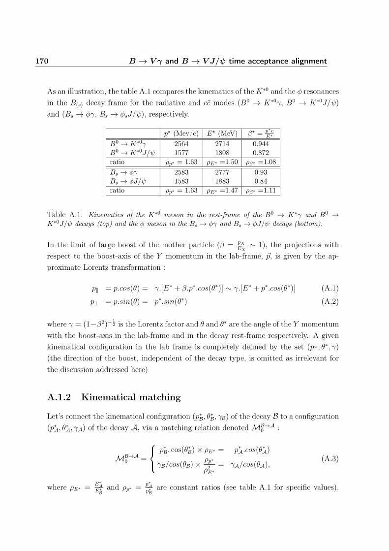
170 B → V γ and B → V J/ψ time acceptance alignment
As an illustration, the table A.1 compares the kinematics of the K∗0 and the φ resonancesin the B(s) decay frame for the radiative and cc modes (B0 → K∗0γ, B0 → K∗0J/ψ)and (Bs → φγ, Bs → φsJ/ψ), respectively.
p (Mev/c) E (MeV) β = p∗cE∗
B0 → K∗0γ 2564 2714 0.944B0 → K∗0J/ψ 1577 1808 0.872ratio ρp∗ = 1.63 ρE∗ =1.50 ρβ∗ =1.08Bs → φγ 2583 2777 0.93Bs → φJ/ψ 1583 1883 0.84ratio ρp∗ = 1.63 ρE∗ =1.47 ρβ∗ =1.11
Table A.1: Kinematics of the K∗0 meson in the rest-frame of the B0 → K∗γ and B0 →K∗0J/ψ decays (top) and the φ meson in the Bs → φγ and Bs → φJ/ψ decays (bottom).
In the limit of large boost of the mother particle (β = pXEX
∼ 1), the projections withrespect to the boost-axis of the Y momentum in the lab-frame, �p, is given by the ap-proximate Lorentz transformation :
p‖ = p.cos(θ) = γ.[E∗ + β.p∗.cos(θ∗)] ∼ γ.[E∗ + p∗.cos(θ∗)] (A.1)
p⊥ = p.sin(θ) = p∗.sin(θ∗) (A.2)
where γ = (1−β2)−12 is the Lorentz factor and θ and θ∗ are the angle of the Y momentum
with the boost-axis in the lab-frame and in the decay rest-frame respectively. A givenkinematical configuration in the lab frame is completely defined by the set (p∗, θ∗, γ)(the direction of the boost, independent of the decay type, is omitted as irrelevant forthe discussion addressed here)
A.1.2 Kinematical matching
Let’s connect the kinematical configuration (p∗B, θ∗B, γB) of the decay B to a configuration
(p∗A, θ∗A, γA) of the decay A, via a matching relation denoted MB→A
0 :
MB→A0 =
⎧⎨⎩ p∗B. cos(θ∗B)× ρE∗ = p∗A.cos(θ
∗A)
γB/cos(θB)× ρp∗
ρ2E∗= γA/cos(θA),
(A.3)
where ρE∗ =E∗
AE∗
Band ρp∗ =
p∗Ap∗B
are constant ratios (see table A.1 for specific values).

A.1 Kinematical basis of the procedure 171
It is worth noticing that in case of an acceptance limited to the very forward region(cos(θA) ∼ cos(θB) ∼ 1), the ratio of the Lorentz factors is essentially independent ofthe angular kinematics : γA/γB ∼ ρp∗/ρ
2E∗ = ρβ∗/ρE∗ .
The Y momenta in the lab-frame for the decays (A) and (B) are related as :
pA.cos(θA) = γA[E∗A + p∗A.cos(θ
∗A)]
= γB[E∗B + p∗B.cos(θ
∗B)]× [
cos(θA)cos(θB)
.ρp∗
ρE∗] = pB.cos(θA)× ρp∗
ρE∗. (A.4)
Combining relations A.3 and A.4 we obtain :
pApB
=ρp∗
ρE∗= ρβ∗ =
cos(θ∗B)cos(θ∗A)
. (A.5)
In other words, the kinematical quantity p.cos(θ∗) is conserved between decays (A) and(B) under the matching relation MB→A
0 in the limit of large boost :
pA.cos(θ∗B) = pB.cos(θ∗A)
The invariance of the transverse momentum with respect to the boost direction (A.2)provides the relation :
sin(θA)sin(θB)
=ρp∗
ρβ∗.sin(θ∗A)sin(θ∗B)
= ρE∗ .sin(θ∗A)sin(θ∗B)
=ρE∗
ρβ∗.
√ρ2β∗ − cos2(θ∗B)√1− cos2(θ∗B)
. (A.6)
The domain of validity of the matching relation and other possible matching choicesare discussed in section A.1.4.
A.1.3 Geometrical matching
In the case of a long-lived particle X, useful relations on the geometrical quantitiesrelying on the decay vertex displacement can be derived from the above kinematicalmatching MB→A
0 . The relevant kinematical and geometrical quantities are reported onthe decay sketch on figure A.1
• Flight distance and related quantitiesThe decay time of the mother particle X being independent of the decay final
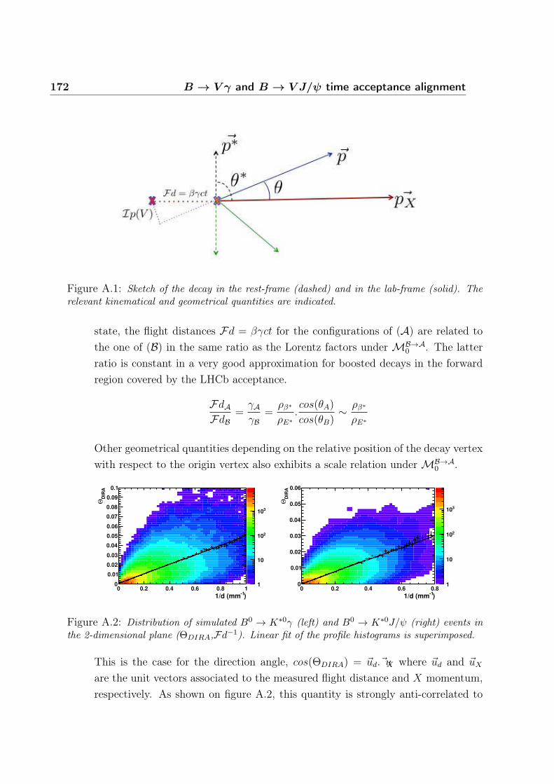
172 B → V γ and B → V J/ψ time acceptance alignment
Figure A.1: Sketch of the decay in the rest-frame (dashed) and in the lab-frame (solid). Therelevant kinematical and geometrical quantities are indicated.
state, the flight distances Fd = βγct for the configurations of (A) are related tothe one of (B) in the same ratio as the Lorentz factors under MB→A
0 . The latterratio is constant in a very good approximation for boosted decays in the forwardregion covered by the LHCb acceptance.
FdAFdB
=γAγB
=ρβ∗
ρE∗.cos(θA)
cos(θB)∼ ρβ∗
ρE∗
Other geometrical quantities depending on the relative position of the decay vertexwith respect to the origin vertex also exhibits a scale relation under MB→A
0 .
Figure A.2: Distribution of simulated B0 → K∗0γ (left) and B0 → K∗0J/ψ (right) events inthe 2-dimensional plane (ΘDIRA,Fd−1). Linear fit of the profile histograms is superimposed.
This is the case for the direction angle, cos(ΘDIRA) = �ud.�uX where �ud and �uX
are the unit vectors associated to the measured flight distance and X momentum,respectively. As shown on figure A.2, this quantity is strongly anti-correlated to

A.1 Kinematical basis of the procedure 173
the flight distance. The average ΘDIRA varies almost linearly with the inverse ofFd. From a linear fit, < ΘDIRA >= α/Fd, of the profile histograms displayed onthe figure A.2, the ratio of slopes α is found to be :
αAαB
= (1.32± 0.01)
for the decay pair (A,B)=(B0 → K∗0γ,B0 → K∗0J/ψ). As a consequence, ΘDIRA
scaling under MB→A0 is roughly expected to be :
< ΘA >
< ΘB >=
αAαB
.FdBFdA
∼ 1.32× ρE∗
ρβ∗∼ 1.84 (A.7)
for that decay pair. Similar behavior is obtained for (A,B)=(Bs → φγ,Bs →φJ/ψ)
Another related quantity, is the isolation vertex variable, Δχ2min, which quantifies
the compatibility of the decay vertex with any other track coming from the originvertex. This variable propagates the same information as the distance of closestapproach of the track with the decay vertex which increases proportionally to theflight distance.
• Impact parametersThe impact parameter of the Y resonance is defined as Ip(Y ) = Fd.sin(θ), leadingto the relation under MB→A
0 :
Ip(Y )AIp(Y )B
=γA.sin(θA)γB.sin(θB)
=ρβ∗
ρE∗.sin(2θA)sin(2θB)
In the limit of small angles in the lab frame and using (A.6) we obtain :
Ip(Y )AIp(Y )B
= ρβ∗ .sin(θ∗A)sin(θ∗B)
= ρβ∗ .
√1− cos2(θ∗B)/ρ
2β∗√
1− cos2(θ∗B). (A.8)
In the case of a large boost in a limited forward acceptance and with ρ2β∗ ∼ 1, theIp(Y ) ratio turns to be approximatively constant :
Ip(Y )AIp(Y )B
∼ ρβ∗ .
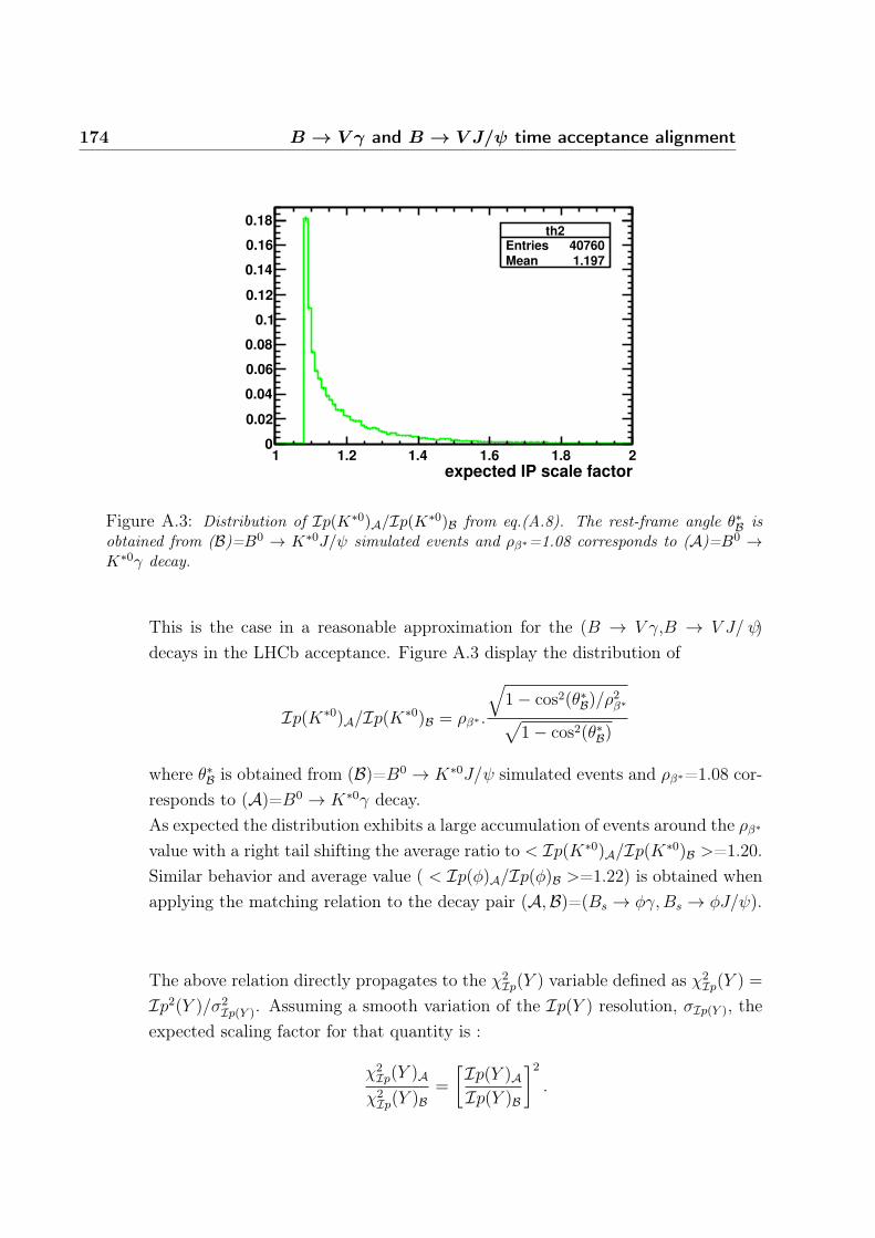
174 B → V γ and B → V J/ψ time acceptance alignment
Figure A.3: Distribution of Ip(K∗0)A/Ip(K∗0)B from eq.(A.8). The rest-frame angle θ∗B isobtained from (B)=B0 → K∗0J/ψ simulated events and ρβ∗=1.08 corresponds to (A)=B0 →K∗0γ decay.
This is the case in a reasonable approximation for the (B → V γ,B → V J/ ψ)decays in the LHCb acceptance. Figure A.3 display the distribution of
Ip(K∗0)A/Ip(K∗0)B = ρβ∗ .
√1− cos2(θ∗B)/ρ
2β∗√
1− cos2(θ∗B)
where θ∗B is obtained from (B)=B0 → K∗0J/ψ simulated events and ρβ∗=1.08 cor-responds to (A)=B0 → K∗0γ decay.As expected the distribution exhibits a large accumulation of events around the ρβ∗
value with a right tail shifting the average ratio to < Ip(K∗0)A/Ip(K∗0)B >=1.20.Similar behavior and average value ( < Ip(φ)A/Ip(φ)B >=1.22) is obtained whenapplying the matching relation to the decay pair (A,B)=(Bs → φγ,Bs → φJ/ψ).
The above relation directly propagates to the χ2Ip(Y ) variable defined as χ2
Ip(Y ) =
Ip2(Y )/σ2Ip(Y ). Assuming a smooth variation of the Ip(Y ) resolution, σIp(Y ), the
expected scaling factor for that quantity is :
χ2Ip(Y )A
χ2Ip(Y )B
=
[Ip(Y )AIp(Y )B
]2.
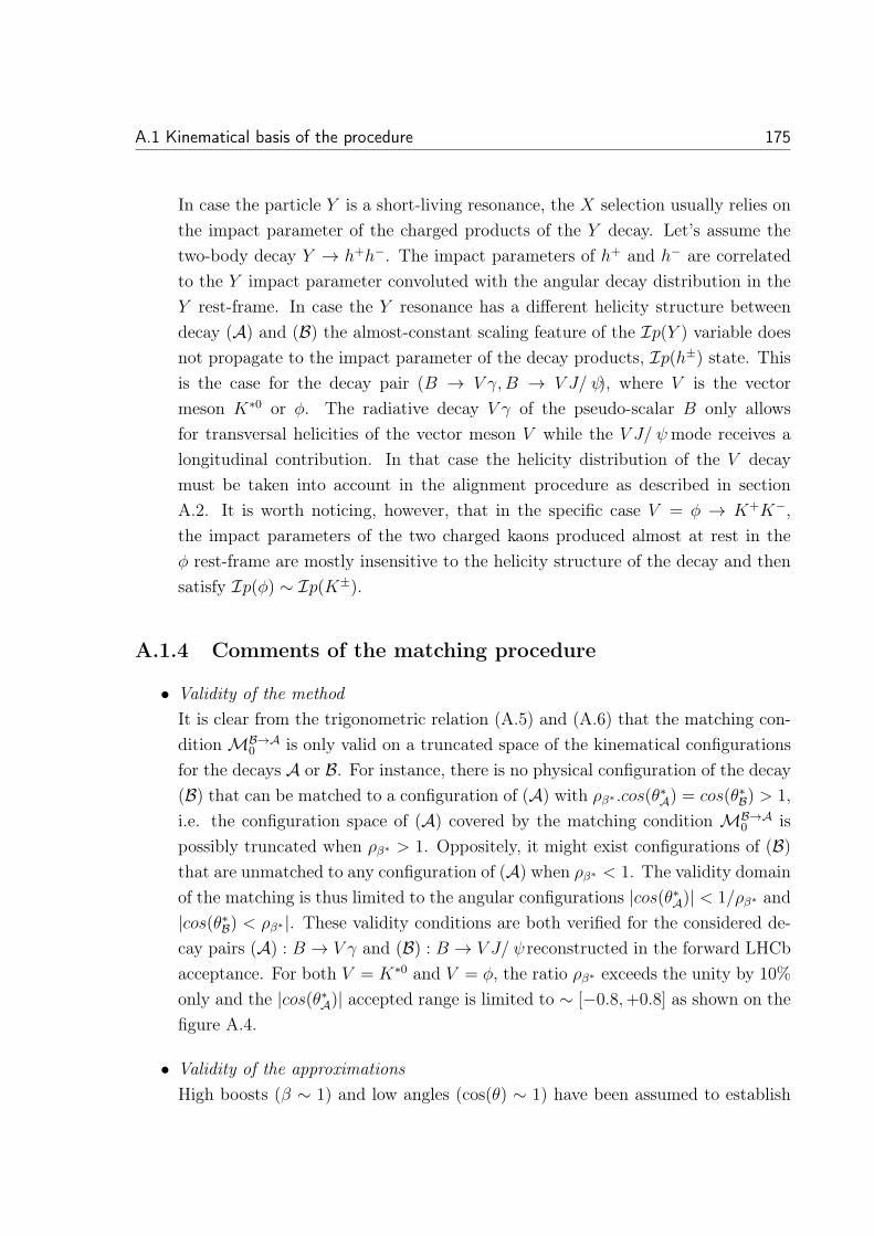
A.1 Kinematical basis of the procedure 175
In case the particle Y is a short-living resonance, the X selection usually relies onthe impact parameter of the charged products of the Y decay. Let’s assume thetwo-body decay Y → h+h−. The impact parameters of h+ and h− are correlatedto the Y impact parameter convoluted with the angular decay distribution in theY rest-frame. In case the Y resonance has a different helicity structure betweendecay (A) and (B) the almost-constant scaling feature of the Ip(Y ) variable doesnot propagate to the impact parameter of the decay products, Ip(h±) state. Thisis the case for the decay pair (B → V γ,B → V J/ ψ), where V is the vectormeson K∗0 or φ. The radiative decay V γ of the pseudo-scalar B only allowsfor transversal helicities of the vector meson V while the V J/ ψmode receives alongitudinal contribution. In that case the helicity distribution of the V decaymust be taken into account in the alignment procedure as described in sectionA.2. It is worth noticing, however, that in the specific case V = φ → K+K−,the impact parameters of the two charged kaons produced almost at rest in theφ rest-frame are mostly insensitive to the helicity structure of the decay and thensatisfy Ip(φ) ∼ Ip(K±).
A.1.4 Comments of the matching procedure
• Validity of the methodIt is clear from the trigonometric relation (A.5) and (A.6) that the matching con-dition MB→A
0 is only valid on a truncated space of the kinematical configurationsfor the decays A or B. For instance, there is no physical configuration of the decay(B) that can be matched to a configuration of (A) with ρβ∗ .cos(θ∗A) = cos(θ∗B) > 1,i.e. the configuration space of (A) covered by the matching condition MB→A
0 ispossibly truncated when ρβ∗ > 1. Oppositely, it might exist configurations of (B)that are unmatched to any configuration of (A) when ρβ∗ < 1. The validity domainof the matching is thus limited to the angular configurations |cos(θ∗A)| < 1/ρβ∗ and|cos(θ∗B) < ρβ∗ |. These validity conditions are both verified for the considered de-cay pairs (A) : B → V γ and (B) : B → V J/ ψ reconstructed in the forward LHCbacceptance. For both V = K∗0 and V = φ, the ratio ρβ∗ exceeds the unity by 10%only and the |cos(θ∗A)| accepted range is limited to ∼ [−0.8,+0.8] as shown on thefigure A.4.
• Validity of the approximationsHigh boosts (β ∼ 1) and low angles (cos(θ) ∼ 1) have been assumed to establish
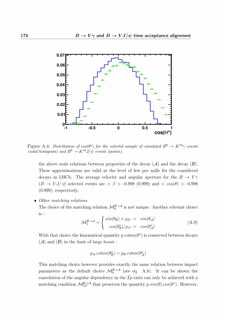
176 B → V γ and B → V J/ψ time acceptance alignment
Figure A.4: Distribution of cos(θ∗) for the selected sample of simulated B0 → K∗0γ events(solid histogram) and B0 → K∗0J/ψ events (points).
the above scale relations between properties of the decay (A) and the decay (B).These approximations are valid at the level of few per mille for the considereddecays in LHCb. The average velocity and angular aperture for the B → V γ
(B → V J/ ψ) selected events are < β >=0.998 (0.999) and < cos(θ) >=0.998(0.999), respectively.
• Other matching relationsThe choice of the matching relation MB→A
0 is not unique. Another relevant choiceis :
MB→A1 =
{sin(θB)× ρE∗ = sin(θA)
cos(θ∗B)/ρβ∗ = cos(θ∗A)(A.9)
With that choice the kinematical quantity p.cotan(θ∗) is conserved between decays(A) and (B) in the limit of large boost :
pA.cotan(θ∗B) = pB.cotan(θ∗A)
This matching choice however provides exactly the same relation between impactparameters as the default choice MB→A
0 (see eq. A.8). It can be shown thecancelation of the angular dependency in the Ip ratio can only be achieved with amatching condition MB→A
IP that preserves the quantity p.sin(θ).cos(θ∗). However,
A.2 Alignment of the proper time acceptance 177
the distributions of this kinematical quantity for the B → V γ and B → V J/ ψ
decays in the LHCb acceptance have a very short overlap and this matching can’tbe used for our time alignement purpose.
A.2 Alignment of the proper time acceptance
The acceptance at low proper time is induced by the selection cuts relying on the B decayvertex displacement (impact parameters, direction angle, ...). In the case of a radiativeB → V γ decay, the vertex decay information is only provided by the charged trackscoming from the decay of the vector meson V . Due to the different decay kinematicsand helicity structure between B → V γ and B → V J/ ψ, the same selection inducesdifferent acceptance. Based on the above discussion on the kinematical matching (A.1)the following three-step procedure is proposed to align the acceptance at low propertime between the two different decays :
• The B → V J/ ψ candidates are reconstructed in such a way the J/ψ → μ+μ−
decays is not used in the decay vertex determination. This is achieved by applyingan arbitrarily large factor to the relevant elements of the covariance matrix of thereconstructed muon tracks. The proper time acceptance is then generated only bythe selection cuts applied on the vector meson and its decay products, as it is forthe corresponding radiative decay.
• An event-by-event reweighing is applied on the B → V J/ ψ sample to statisticallyreproduce the B → V γ distribution in the two-dimensional plane (p.cos(θ∗),θH),where θH is the helicity angle of the V decay. The reweighing in the first direction(p.cos(θ∗)) aims at aligning the kinematics according to the matching relationMB→A
0 discussed above while the helicity reweighing accounts for the differenthelicity-structure of the V decay.
• After the reweighing, the two different decays are assumed to exhibits almost-constant ratios for the vertex-related variables that induces the low proper timeacceptance. A scaling factor is extracted for the relevant variables and the corre-sponding selection cuts are scaled accordingly.

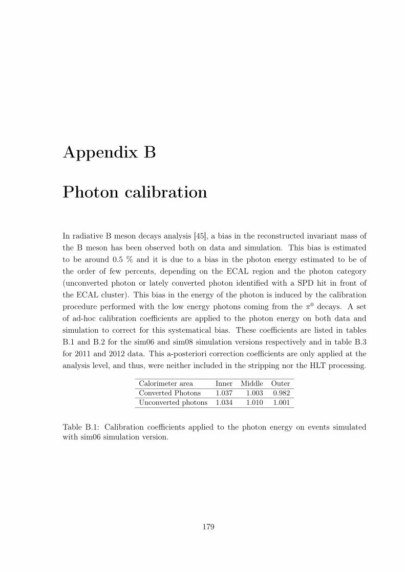
Appendix B
Photon calibration
In radiative B meson decays analysis [45], a bias in the reconstructed invariant mass ofthe B meson has been observed both on data and simulation. This bias is estimatedto be around 0.5 % and it is due to a bias in the photon energy estimated to be ofthe order of few percents, depending on the ECAL region and the photon category(unconverted photon or lately converted photon identified with a SPD hit in front ofthe ECAL cluster). This bias in the energy of the photon is induced by the calibrationprocedure performed with the low energy photons coming from the π0 decays. A setof ad-hoc calibration coefficients are applied to the photon energy on both data andsimulation to correct for this systematical bias. These coefficients are listed in tablesB.1 and B.2 for the sim06 and sim08 simulation versions respectively and in table B.3for 2011 and 2012 data. This a-posteriori correction coefficients are only applied at theanalysis level, and thus, were neither included in the stripping nor the HLT processing.
Calorimeter area Inner Middle OuterConverted Photons 1.037 1.003 0.982Unconverted photons 1.034 1.010 1.001
Table B.1: Calibration coefficients applied to the photon energy on events simulatedwith sim06 simulation version.
179

180 Photon calibration
Calorimeter area Inner Middle OuterConverted Photons 1.044 1.010 0.989Unconverted photons 1.041 1.017 1.008
Table B.2: Calibration coefficients applied to the photon energy on events simulatedwith sim08 simulation version.
Calorimeter area Inner Middle OuterConverted Photons 1.019 0.999 0.959Unconverted photons 1.001 0.994 0.976
Table B.3: Calibration coefficients applied to the photon energy on 2011 and 2012 datasamples.
Appendix C
Definition of the different variablesused for selections
The definitions of the different variables used for the selection are introduced here
• The flight distance (Fd) is the distance covered by the reconstructed B mesonfrom its creation at the interaction point, named primary vertex (PV), to thepoint where it decays, named secondary vertex (SV). The flight distance is relatedto the proper time of the B meson through Fd = βγct where β and γ are theLorentz factors, c is the speed of light and t is the proper time of the B meson.
• The DIRection Angle, θDIRA, is the angle between the line connecting the PVand the SV and the direction of the momentum of the B meson. It is given ascos(ΘDIRA) = �u.�v where �u and �v are the unit vectors associated to the measuredflight distance direction and B momentum, respectively.
• The Impact Parameter (IP) of a given track x relative to a PV is the distanceof closest approach between the extrapolated track and the PV. It is defined asIP = Fd.sin(θx) where θx is the angle defined by the track x and the flight distancedirection.
• η is the pseudo rapidity defined as η = −ln(tan(θ/2)) with θ being the anglebetween the momentum of the particle and the beam axis.
• P is the momentum of a given particle.
• ET is the transverse energy with respect to the beam line: ET = E sin θ.
181

182 Definition of the different variables used for selections
• PT is the transverse momentum of a given particle with respect to the beam line:PT = P sin θ
• γ/π0 separation is the output variable from the classifier trained to separate pho-tons from merged π0 discussed in 3.5.
• γCL is the photon confidence level. This variable is a transformation in the [0,1]range of the likelihood estimator discussed in 3.4.1 .
• In the selection cuts, M refers to the mass and ΔM refers to a mass range.
• The vertex χ2 of a reconstructed resonance quantifies the compatibility of thetracks to decay from vertex.
• The vertex isolation cut of the B, Δχ2, quantifies the compatibility of the decayvertex with any other track not associated with the decay’s tracks.
• ZPV is the z coordinate of the B reconstructed vertex.
• nPV is the number of reconstructed primary vertices in the event.
• IPχ2next quantifies the compatibility of a given b hadron with the second most
probable PV that it can be associated with.
• The helicity angle for B → (V → h+h−)γ decay, θH is the angle between themomentum of the B and the momentum of h+ in h+ rest frame.
• The Particle IDentification (PID) variables for charged particles exist in two ver-sion:
– Variables named ProbNN rely on the Neural Net (NN) procedure imple-mented at LHCb in 2012 (explained briefly in chapter 2.3.7) and are usedas: xProbNNx(y) is the hypothesis of identifying (misidentifying) x as beingx (y).
– Variables named PID rely on the ΔLL procedure implemented since the startof LHCb (explained briefly in chapter 2.3.7) and are used as: xPIDx(y) is thehypothesis of identifying (misidentifying) x as being x (y).
• The ghost probability of a track is the probability for this track to be reconstructedfrom hits in the tracking system that belong to two separate tracks.

183
• isMuon is a veto applied to select true muons. The veto is defined by the numberof hits in the muon stations.

Bibliography
[1] S.L. Glashow. Partial Symmetries of Weak Interactions. Nucl.Phys., 22:579–588,1961.
[2] Steven Weinberg. The Quantum Theory of fields, volume I: Foundations. Cam-bridge University Press., May 2005.
[3] F. Englert and R. Brout. Broken Symmetry and the Mass of Gauge Vector Mesons.Phys. Rev. Lett., 13:321–323, Aug 1964.
[4] G. S. Guralnik, C. R. Hagen, and T. W. B. Kibble. Global conservation laws andmassless particles. Phys. Rev. Lett., 13:585–587, Nov 1964.
[5] Peter W. Higgs. Broken symmetries and the masses of gauge bosons. Phys. Rev.Lett., 13:508–509, Oct 1964.
[6] Peter W. Higgs. Spontaneous symmetry breakdown without massless bosons. Phys.Rev., 145:1156–1163, May 1966.
[7] Georges Aad et al. Observation of a new particle in the search for the StandardModel Higgs boson with the ATLAS detector at the LHC. Phys.Lett., B716:1–29,2012.
[8] Serguei Chatrchyan et al. Observation of a new boson at a mass of 125 GeV withthe CMS experiment at the LHC. Phys.Lett., B716:30–61, 2012.
[9] Nicola Cabibbo. Unitary Symmetry and Leptonic Decays. Phys.Rev.Lett., 10:531–533, 1963.
[10] Makoto Kobayashi and Toshihide Maskawa. CP Violation in the RenormalizableTheory of Weak Interaction. Prog.Theor.Phys., 49:652–657, 1973.
185
186 BIBLIOGRAPHY
[11] Patricia Ball, Gareth W. Jones, and Roman Zwicky. b → vγ beyond qcd factor-ization. Phys. Rev. D, 75:054004, Mar 2007.
[12] Benjamin Grinstein, Yuval Grossman, Zoltan Ligeti, and Dan Pirjol. Photonpolarization in b → xγ in the standard model. Phys. Rev. D, 71:011504, Jan 2005.
[13] Matthias Neubert. Radiative b decays: Standard candles of flavor physics. pages252–264, 2002.
[14] Tobias Hurth. Present status of inclusive rare b decays. Rev. Mod. Phys., 75:1159–1199, Oct 2003.
[15] A. Ali, B.D. Pecjak, and C. Greub. Towards b → vγ decays at nnlo in scet. TheEuropean Physical Journal C, 55(4):577–595, 2008.
[16] Mikocaj Misiak and Matthias Steinhauser. Three-loop matching of the dipoleoperators. Nuclear Physics B, 683(1–2):277 Р305, 2004.
[17] Martin Gorbahn and Ulrich Haisch. Effective hamiltonian for non-leptonic decaysat {NNLO} in {QCD}. Nuclear Physics B, 713(1–3):291 Р332, 2005.
[18] Michal Czakon, Ulrich Haisch, and Mikolaj Misiak. Four-Loop Anomalous Dimen-sions for Radiative Flavour-Changing Decays. JHEP, 0703:008, 2007.
[19] Benjamin Grinstein and Dan Pirjol. cp asymmetry in b0(t) → kSπ0γ in the stan-
dard model. Phys. Rev. D, 73:014013, Jan 2006.
[20] Lisa L. Everett, Gordon L. Kane, S. Rigolin, Lian-Tao Wang, and Ting T. Wang.Alternative approach to b → sγ in the uMSSM. JHEP, 0201:022, 2002.
[21] Michael Gronau, Yuval Grossman, Dan Pirjol, and Anders Ryd. Measuring thephoton polarization in B → Kππγ. Phys.Rev.Lett., 88:051802, 2002.
[22] Michael Gronau and Dan Pirjol. Photon polarization in radiative B decays.Phys.Rev., D66:054008, 2002.
[23] Aaij et al. Observation of photon polarization in the b → sγ transition. Phys.Rev. Lett., 112(arXiv:1402.6852. CERN-PH-EP-2014-026. LHCB-PAPER-2014-001):161801. 17 p, Feb 2014.
[24] V. Orlovsky and V. Shevchenko. Photon polarization in radiative b → φkγ decay.Phys. Rev. D, 77:093003, May 2008.
BIBLIOGRAPHY 187
[25] D. Melikhov, N. Nikitin, and S. Simula. Probing right-handed currents in B →K∗l+l− transitions. Phys.Lett., B442:381–389, 1998.
[26] C. Kim, Yeong Kim, Cai-Dian Lü, and Takuya Morozumi. Azimuthal angle dis-tribution in b → k∗(→ kπ)l+l− in the low invariant ml+l− region. Phys. Rev. D,62:034013, Jul 2000.
[27] Yuval Grossman and Dan Pirjol. Extracting and using photon polarization in-formation in radiative b decays. Journal of High Energy Physics, 2000(06):029,2000.
[28] Frank Krüger, Lalit Sehgal, Nita Sinha, and Rahul Sinha. Angular distributionand CP asymmetries in the decays B → K−π+e−e+ and B → π−π+e−e+. Phys.Rev. D, 61:114028, May 2000.
[29] J Lefrançois and M H Schune. Measuring the photon polarization in b → sγ
using the B → K∗e+e− decay channel. Technical Report LHCb-PUB-2009-008.CERN-LHCb-PUB-2009-008. LHCb-INT-2009-007, CERN, Geneva, Jun 2009.
[30] Aaij et al. Measurement of the b → k∗(892)0e+e− branching fraction at lowdilepton mass. Journal of High Energy Physics, 2013(5), 2013.
[31] Aaij et al. Angular analysis of the decay b → k∗(892)0e+e− in the low-q2 region.2015.
[32] Damir Becirevic and Elia Schneider. On transverse asymmetries in b → k∗l+l−.Nuclear Physics B, 854(2):321 – 339, 2012.
[33] David Atwood, Tim Gershon, Masashi Hazumi, and Amarjit Soni. Mixing-inducedcp violation in b → P1P2γ in search of clean new physics signals. Phys. Rev. D,71:076003, Apr 2005.
[34] J. Beringer et al. Review of particle physics. Phys. Rev. D, 86:010001, Jul 2012.
[35] Bernard Aubert et al. Measurement of Time-Dependent CP Asymmetry in B0 →K0
Sπ0γ Decays. Phys.Rev., D78:071102, 2008.
[36] Y. Ushiroda et al. Time-Dependent CP Asymmetries in B0 → K0Sπ
0γ transitions.Phys.Rev., D74:111104, 2006.
188 BIBLIOGRAPHY
[37] Franz Muheim, Yuehong Xie, and Roman Zwicky. Exploiting the width differencein bs → φγ. Physics Letters B, 664(3):174–179, 2008.
[38] Thomas Mannel and Stefan Recksiegel. Flavour-changing neutral current decaysof heavy baryons. Journal of Physics G: Nuclear and Particle Physics, 24(5):979,1998.
[39] Gudrun Hiller and Alex Kagan. Probing for new physics in polarized Lambda(b)decays at the Z. Phys.Rev., D65:074038, 2002.
[40] Federica Legger and Thomas Schietinger. Photon helicity in Λb → pKγ decays.Phys.Lett., B645:204–212, 2007.
[41] G. Hiller T. Blake, T. Gershon. Rare b hadron decays at the lhc. 2015.
[42] R Aaij et al. Measurements of the Λ0b → J/ψΛ decay amplitudes and the Λ0
b
polarisation in pp collisions at√s = 7 TeV. Phys.Lett., B724:27–35, 2013.
[43] D. Bef çirevif á, E. Kou, A. Le Yaouanc, and A. Tayduganov. Future prospects forthe determination of the wilson coefficient c′7γ . Journal of High Energy Physics,2012(8), 2012.
[44] Bharucha et al. Implications of lhcb measurements and future prospects. TheEuropean Physical Journal C, 73(4), 2013.
[45] R Aaij et al. Measurement of the ratio of branching fractions BR(B0 -> K*0gamma)/BR(Bs0 -> phi gamma) and the direct CP asymmetry in B0 -> K*0gamma. Nucl.Phys., B867:1–18, 2013.
[46] B. Adeva et al. Roadmap for selected key measurements of LHCb. 2009.
[47] Lyndon Evans and Philip Bryant. Lhc machine. Journal of Instrumentation,3(08):S08001, 2008.
[48] The LHCb Collaboration. Absolute luminosity measurements with the lhcb de-tector at the lhc. Journal of Instrumentation, 7(01):P01010, 2012.
[49] R Aaij et al. Measurement of B meson production cross-sections in proton-protoncollisions at
√s = 7 TeV. J. High Energy Phys., 08(arXiv:1306.3663. CERN-PH-
EP-2013-095. LHCB-PAPER-2013-004):117. 13 p, Jul 2013. Comments: 13 pages,12 figures, 1 table, submitted to JHEP.
BIBLIOGRAPHY 189
[50] A. Augusto Alves et al. The LHCb Detector at the LHC. JINST, 3:S08005, 2008.
[51] M. Adinolfi et al. Performance of the lhcb rich detector at the lhc. The EuropeanPhysical Journal C, 73(5), 2013.
[52] C Abellan Beteta et al. Time alignment of the front end electronics of the lhcbcalorimeters. Journal of Instrumentation, 7(08):P08020, 2012.
[53] Irina Machikhiliyan and the LHCb calorimeter group. Current status and perfor-mance of the lhcb electromagnetic and hadron calorimeters. Journal of Physics:Conference Series, 293(1):012052, 2011.
[54] J Lefrançois, F Machefert, and A Martens. Calibration of the LHCb calorimeterswith energy flow. Technical Report LHCb-INT-2010-021. CERN-LHCb-INT-2010-021, CERN, Geneva, Apr 2010.
[55] Ivan Belyaev, Victor Egorychev, and Daria Savrina. ECAL calibration within Kaliframework: A Mass distribution fit‚ A method calibration with the real data. Tech-nical Report LHCb-INT-2011-049. CERN-LHCb-INT-2011-049, CERN, Geneva,Oct 2011.
[56] A Arefev, S Barsuk, I Belyaev, B Bobchencko, L Camilleri, V Egorychev, Yu Gilit-sky, A Golutvin, O Gouchtchine, I Korolko, T Kvaratskheliia, I Machikhilian,M Martemyanov, E Melnikov, A Morozov, M Prokudin, D Roussinov, V Rusinov,A Schopper, S Schuvalov, A Soldatov, E Tarkovski, and K Voronchev. Beam TestResults of the LHCb Electromagnetic Calorimeter. Technical Report LHCb-2007-149. CERN-LHCb-2007-149, CERN, Geneva, May 2008. revised version submittedon 2008-05-15 09:09:53.
[57] Andrew Powell. Reconstruction and PID performance of the LHCb RICH detec-tors. Nucl.Instrum.Meth., A639:260–263, 2011.
[58] Antunes-Nobrega et al. LHCb trigger system: Technical Design Report. TechnicalDesign Report LHCb. CERN, Geneva, 2003. revised version number 1 submittedon 2003-09-24 12:12:22.
[59] Vladimir V Gligorov. A single track HLT1 trigger. Technical Report LHCb-PUB-2011-003. CERN-LHCb-PUB-2011-003. LHCb-INT-2010-053, CERN, Geneva, Jan2011.
190 BIBLIOGRAPHY
[60] Roel Aaij and Johannes Albrecht. Muon triggers in the High Level Triggerof LHCb. Technical Report LHCb-PUB-2011-017. CERN-LHCb-PUB-2011-017,CERN, Geneva, Sep 2011.
[61] M Williams, Vladimir V Gligorov, C Thomas, H Dijkstra, J Nardulli, andP Spradlin. The HLT2 Topological Lines. Technical Report LHCb-PUB-2011-002. CERN-LHCb-PUB-2011-002, CERN, Geneva, Jan 2011.
[62] Byron P. Roe, Hai-Jun Yang, Ji Zhu, Yong Liu, Ion Stancu, et al. Boosted decisiontrees, an alternative to artificial neural networks. Nucl.Instrum.Meth., A543:577–584, 2005.
[63] S Tolk, J Albrecht, F Dettori, and A Pellegrino. Data driven trigger efficiencydetermination at LHCb. Technical Report LHCb-PUB-2014-039. CERN-LHCb-PUB-2014-039, CERN, Geneva, May 2014.
[64] Albert Puig Navarro and Ricardo Graciani Diaz. First measurements of radiativeB decays in LHCb. PhD thesis, Barcelona U., 2012. Presented 09 Mar 2012.
[65] Aaij et al. Absolute luminosity measurements with the LHCb detector at theLHC. J. Instrum., 7(arXiv:1110.2866. LHCB-PAPER-2011-015. CERN-PH-EP-2011-157):P01010. 47 p, Oct 2011.
[66] Roel Aaij et al. Precision luminosity measurements at LHCb. JINST, 9:12005,2014.
[67] P Mato. GAUDI-Architecture design document. Technical Report LHCb-98-064,CERN, Geneva, Nov 1998.
[68] G. Barrand, I. Belyaev, P. Binko, M. Cattaneo, R. Chytracek, et al. GAUDI -A software architecture and framework for building HEP data processing applica-tions. Comput.Phys.Commun., 140:45–55, 2001.
[69] Antunes-Nobrega et al. LHCb computing: Technical Design Report. TechnicalDesign Report LHCb. CERN, Geneva, 2005. Submitted on 11 May 2005.
[70] R. Brun and F. Rademakers. ROOT: An object oriented data analysis framework.Nucl.Instrum.Meth., A389:81–86, 1997.
[71] The root project. http://root.cern.ch/.
BIBLIOGRAPHY 191
[72] I. Belyaev, P. Charpentier, S. Easo, P. Mato, J. Palacios, et al. Simulation appli-cation for the LHCb experiment. eConf, C0303241:TUMT003, 2003.
[73] I Belyaev, T Brambach, N H Brook, N Gauvin, G Corti, K Harrison, P F Harri-son, J He, P H Hilten, C R Jones, M Lieng, G Manca, S Miglioranzi, P Robbe,V Vagnoni, M Whitehead, and J Wishahi. Handling of the generation of primaryevents in Gauss, the LHCb simulation framework. Nov 2010.
[74] Torbjorn Sjostrand, Stephen Mrenna, and Peter Z. Skands. PYTHIA 6.4 Physicsand Manual. JHEP, 0605:026, 2006.
[75] D.J. Lange. The EvtGen particle decay simulation package. Nucl.Instrum.Meth.,A462:152–155, 2001.
[76] Elisabetta Barberio, Bob van Eijk, and Zbigniew Was. PHOTOS: A UniversalMonte Carlo for QED radiative corrections in decays. Comput.Phys.Commun.,66:115–128, 1991.
[77] S. Agostinelli et al. GEANT4: A Simulation toolkit. Nucl.Instrum.Meth.,A506:250–303, 2003.
[78] The LHCb collaboration. The boole project. http://lhcb-release-area.web.cern.ch/LHCb-release-area/DOC/boole/.
[79] The LHCb collaboration. The brunel project. http://lhcb-release-area.web.cern.ch/LHCb-release-area/DOC/brunel/.
[80] The LHCb collaboration. The moore project. http://lhcb-release-area.web.cern.ch/LHCb-release-area/DOC/moore/.
[81] The LHCb collaboration. The davinci project. http://lhcb-release-area.web.cern.ch/LHCb-release-area/DOC/davinci/.
[82] O Callot. Calorimeter data format and 2-D zero suppression scheme. TechnicalReport LHCb-99-037, CERN, Geneva, Oct 1999.
[83] V. Breton, N. Brun, and P. Perret. A clustering algorithm for the LHCb electro-magnetic calorimeter using a cellular automaton. 2001.
[84] R. Hollebeek. Topics in calorimetry for high-energy physics. 1991.
192 BIBLIOGRAPHY
[85] O. Deschamps, F.P. Machefert, M.H. Schune, G. Pakhlova, and I. Belyaev. Photonand neutral pion reconstruction. 2003.
[86] K.A. Olive et al. Review of Particle Physics. Chin.Phys., C38:090001, 2014.
[87] Diego Alejandro Roa Romero and Pascal Perret. Study of charmless B0d,s →
h+h′−π0 decays in LHCb. PhD thesis, Clermont-Ferrand U., May 2013. Presented24 May 2013.
[88] OLIVIER DESCHAMPS. Recherche du boson de higgs du modele standard mini-mal dans les etats finals hadroniques avec le detecteur aleph a lep 2. PhD thesis,1999. Thèse de doctorat dirigée par Gay, Pascal Physique Clermont Ferrand 21999.
[89] F P Machefert. Photon Identification. Technical Report LHCb-2004-032, CERN,Geneva, Apr 2004.
[90] Krzysztof Grzegorz Sobczak. Study of charmless three-body decays of neutral Bmesons with the LHCb spectrometer. PhD thesis, 2011. 2011CLF22202.
[91] Andreas Hoecker, Peter Speckmayer, Joerg Stelzer, Jan Therhaag, Eckhard vonToerne, and Helge Voss. TMVA: Toolkit for Multivariate Data Analysis. PoS,ACAT:040, 2007.
[92] G. W. Corder and D. I. Foreman. onparametric Statistics for Non-Statisticians:A Step-by-Step Approach. John Wiley and Sons, Inc., 2009.
[93] Lior Rokach and Oded Z Maimon. Data mining with decision trees: theory andapplications, volume 69. World Scientific Pub Co Inc, 2008.
[94] L Shchutska, A Golutvin, and I Belyaev. "Study of radiative penguin decaysB → K∗0γ and Bs → φγ at LHCb". Technical Report LHCb-2007-030. CERN-LHCb-2007-030, CERN, Geneva, May 2007.
[95] Muriel Pivk and Francois R. Le Diberder. SPlot: A Statistical tool to unfold datadistributions. Nucl.Instrum.Meth., A555:356–369, 2005.
[96] Heavy Flavor Averaging Group. Averages of b-hadron, c-hadron, and τ -leptonproperties as of summer 2014. 2014.
BIBLIOGRAPHY 193
[97] b-hadron lifetime measurements with exclusive b → J/ψX decays reconstructed inthe 2010 data. Mar 2011. LHCb-ANA-2011-001.
[98] Roel Aaij et al. Measurement of the B+c meson lifetime using B+
c → J/ψμ+νμX
decays. Eur.Phys.J., C74(5):2839, 2014.
[99] The roofit project. https://root.cern.ch/drupal/content/roofit.
[100] R. Aaij et al. Measurement of the ratio of branching fractions B(B0 →K∗0γ)/B(B0
s → φγ) and the direct CP asymmetry in B0 → K∗0γ. Nucl. Phys.,B867:1–18, 2013.
[101] Argus Collaboration. Search for hadronic b → u decays. Physics Letters B,241:278–282, May 1990.
[102] M. Oreglia. A Study of the Reactions ψ′ → γγψ. 1980.
[103] D. Martinez Santos and F. Dupertuis. Mass distributions marginalized over per-event errors. Nuclear Instruments and Methods in Physics Research Section A:Accelerators, Spectrometers, Detectors and Associated Equipment, 764(0):150 –155, 2014.
[104] LHCb collaboration. A package for extracting pid performance from data and mc.https://twiki.cern.ch/twiki/bin/view/LHCb/PIDCalibPackage.
[105] Fatima Soomro. Radiative decays of B mesons at LHCb. PhD thesis.
[106] Roel Aaij et al. Measurements of the B+, B0, B0s meson and Λ0
b baryon lifetimes.JHEP, 1404:114, 2014.
[107] O. Callot. FastVelo, a fast and efficient pattern recognition package for the Velo.September 2011.
[108] K. Wyllie, F. Alessio, R. Jacobsson, and N. Neufeld. Electronics Architecture ofthe LHCb Upgrade. 2011.
[109] Aaij et al. Measurement of the B0 − B0 and B0s − B0
s production asymmetries inpp collisions at
√s = 7 TeV. Phys. Lett. B, 739(arXiv:1408.0275. CERN-PH-EP-
2014-181. LHCB-PAPER-2014-042):218. 24 p, Aug 2014. Comments: Updated tov2 after journal review.

Résumé
Cette thèse est dédiée à l’étude des désintégrations B0s → φγ au LHCb afin de mesurer la
polarisation du photon . Au niveau des quarks, ces désintégrations procèdent via une transitionpingouin b → sγ et sont sensibles aux eventuelles contributions virtuelles de Nouvelle Physique.La mesure de la polarisation du photon permet de tester la structure V − A du couplage duModèle Standard dans les processus des diagrammes de boucles de pingouin. Cette mesurepeut être réalisée en étudiant le taux de désintégration dépendant du temps des mésons B. Uneanalyse délicate a été faite pour comprendre la distribution du temps propre et l’acceptancede sélection qui affecte cette distribution. Afin de contrôler l’acceptance de temps propre,des méthodes basées sur les données ont été développées. Plusieurs stratégies utilisées dansla mesure de la polarisation des photons sont introduites et des résultats préliminaires sontprésentés. De plus, une étude de certains effets systématiques est discutée. Dans le cadrede l’étude des désintégrations radiatives, une nouvelle procedure d’identification de photonsa été développée et nous avons fourni un outil pour calibrer la performance de la variablede séparation photon/pion neutre sur la simulation. Ces outils sont d’intérêt général pour lacollaboration LHCb et sont largement utilisés.
Abstract
This thesis is dedicated to the study of the photon polarization in B0s → φγ decays at LHCb.
At the quark level, such decays proceed via a b → sγ penguin transition and are sensitive topossible virtual contributions from New Physics. The measurement of the photon polarizationstands also as a test of the V − A structure of the Standard Model coupling in the processesmediated by loop penguin diagrams. The measurement of the photon polarization can be donethrough a study of the time-dependent decay rate of the B meson. A delicate treatment hasbeen done to understand the proper time distribution and the selection acceptance affectingit. To control the proper time acceptance, data driven control methods have been developed.Several possible strategies to measure the photon polarization are introduced and preliminaryblinded results are presented. A study of some of the systematic effects is discussed. In thecontext of studying radiative decays, the author has developed a new photon identificationprocedure and has provided a tool to calibrate the performance of the photon/neutral pion sep-aration variable on simulation. Those tools are of general interest for the LHCb collaborationand are widely used.
Keywords: LHCb detector - Heavy Flavor Physics - Radiative Decays - EffectiveField Theories - B0
s → φγ - Photon Polarization - Proper Time - Photon Identifi-cation - γ/π0 separation.