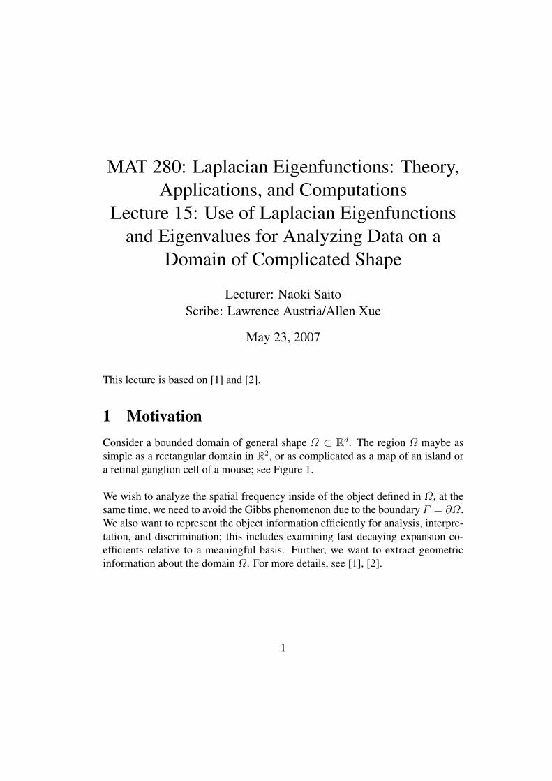
MAT 280: Laplacian Eigenfunctions: Theory,Applications, and Computations

Lecture 15: Use of Laplacian Eigenfunctionsand Eigenvalues for Analyzing Data on a

Domain of Complicated Shape

Lecturer: Naoki SaitoScribe: Lawrence Austria/Allen Xue

May 23, 2007

This lecture is based on [1] and [2].

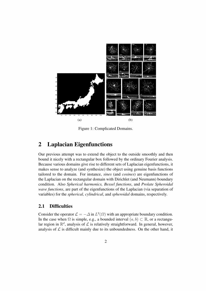
1 MotivationConsider a bounded domain of general shape Ω ⊂ Rd. The region Ω maybe assimple as a rectangular domain in R2, or as complicated as a map of an island ora retinal ganglion cell of a mouse; see Figure 1.

We wish to analyze the spatial frequency inside of the object defined in Ω, at thesame time, we need to avoid the Gibbs phenomenon due to the boundary Γ = ∂Ω.We also want to represent the object information efficiently for analysis, interpre-tation, and discrimination; this includes examining fast decaying expansion co-efficients relative to a meaningful basis. Further, we want to extract geometricinformation about the domain Ω. For more details, see [1], [2].

1

10 20 30 40 50 60 70 80 90 100

10

20

30

40

50

60

70

80

90

(a) (b)

Figure 1: Complicated Domains.

2 Laplacian EigenfunctionsOur previous attempt was to extend the object to the outside smoothly and thenbound it nicely with a rectangular box followed by the ordinary Fourier analysis.Because various domains give rise to different sets of Laplacian eigenfunctions, itmakes sense to analyze (and synthesize) the object using genuine basis functionstailored to the domain. For instance, sines (and cosines) are eigenfunctions ofthe Laplacian on the rectangular domain with Dirichlet (and Neumann) boundarycondition. Also Spherical harmonics, Bessel functions, and Prolate Spheroidalwave functions, are part of the eigenfunctions of the Laplacian (via separation ofvariables) for the spherical, cylindrical, and spheroidal domains, respectively.

2.1 DifficultiesConsider the operator L = −∆ in L2(Ω) with an appropriate boundary condition.In the case when Ω is simple, e.g., a bounded interval (a, b) ⊂ R, or a rectangu-lar region in Rd, analysis of L is relatively straightforward. In general, however,analysis of L is difficult mainly due to its unboundedness. On the other hand, it

2

is much better to analyze its inverse, i.e., the Green’s operator because it is com-pact and self-adjoint. Thus L−1 has discrete spectra (i.e., countable number ofeigenvalues with finite multiplicity) except for the 0 spectrum. We use the factthat L induces a complete orthonormal basis for L2(Ω) to allow us to performeigenfunction expansion in L2(Ω). Another difficulty is computing such eigen-functions; directly solving the Helmholtz equation (or the Laplacian eigenvalueproblem) on a general domain Ω is tough. In addition, computing the Green’sfunction for a general Ω satisfying the usual boundary conditions (e.g., Dirichletor Neumann) is very difficult too.

3 Integral Operators Commuting with the Lapla-cian

Instead of computing the eigenfunctions of L on a general domain, we look atcertain integral operators commuting with L. The key idea is to find an integraloperator commuting with the Laplacian without imposing the strict boundary con-dition a priori. Then we know that the eigenfunctions of the Laplacian is the sameas those of the integral operator, which is much easier to deal with–thanks to thefollowing fact:

Theorem 3.1 (G. Frobenius 1878?; B. Friedman 1956). Suppose K and L com-mute and one of them has an eigenvalue with finite multiplicity. Then K and Lshare the same eigenfunction corresponding to that eigenvalue. That is, Lϕ = λϕand Kϕ = µϕ.

Now, let’s replace the Green’s function G(x, y) by the fundamental solution ofthe Laplacian:

K(x,y) =

−12|x− y| for d = 1

− 12π

log |x− y| for d = 2

1(d−2)ωd

|x− y|2−d for d > 2

where ωd is the surface area of the d-dimensional unit ball. The price we pay is tohave a rather implicit, non-local boundary condition (although we do not need todeal with this condition directly). Let K be the integral operator whose kernel isK, i.e., for all f ∈ L2(Ω), define:

3

K(f(x)) ,∫

Ω

K(x,y)f(y) dy.

On the other hand, what we gain are the following:

Theorem 3.2. The integral operator K commutes with the Laplacian L = −∆with the following non-local boundary condition:

∫

Γ

K(x,y)∂ϕ

∂νy

(y) ds(y) = −1

2ϕ(x) + pv

∫

Γ

∂K(x,y)

∂νy

ϕ(y) ds(y)

for all x ∈ Γ = ∂Ω, where ϕ is an eigenfunction common for both operators.

Corollary 3.3. The integral operator K is compact and self-adjoint in L2(Ω).Thus the kernel K(x,y) had the following eigenfunction expansion (in the senseof mean convergence):

K(x, y) ∼∞∑

j=1

µjϕj(x)ϕj(y)

and ϕj∞j=1 forms an orthonormal basis of L2(Ω)

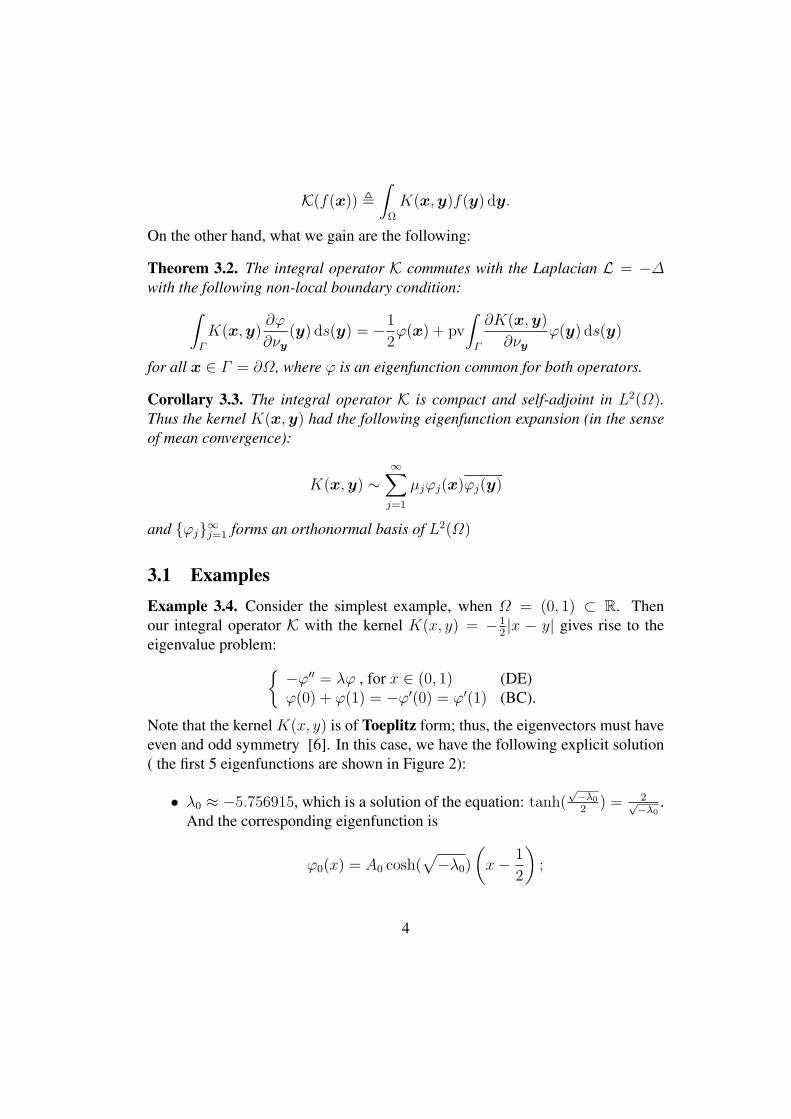
3.1 ExamplesExample 3.4. Consider the simplest example, when Ω = (0, 1) ⊂ R. Thenour integral operator K with the kernel K(x, y) = −1

2|x − y| gives rise to the

eigenvalue problem: −ϕ′′ = λϕ , for x ∈ (0, 1) (DE)

ϕ(0) + ϕ(1) = −ϕ′(0) = ϕ′(1) (BC).

Note that the kernel K(x, y) is of Toeplitz form; thus, the eigenvectors must haveeven and odd symmetry [6]. In this case, we have the following explicit solution( the first 5 eigenfunctions are shown in Figure 2):

• λ0 ≈ −5.756915, which is a solution of the equation: tanh(√−λ0

2) = 2√−λ0

.And the corresponding eigenfunction is

ϕ0(x) = A0 cosh(√−λ0)

(x− 1

2

);

4

0 0.1 0.2 0.3 0.4 0.5 0.6 0.7 0.8 0.9 1−0.06

−0.04

−0.02

0

0.02

0.04

0.06

Figure 2: First 5 eigenfunctions.

• λ2m−1 = (2m− 1)2π2 for all m ∈ N, and the corresponding eigenfunctionis

ϕ2m−1(x) =√

2 cos(2m− 1)πx;

• λ2m for all m ∈ N is a solution of the equation: tan√

λ2m

2= − 2√

λ2m, and

the corresponding eigenfunction is

ϕ2m(x) = A2m cos√

λ2m

(x− 1

2

).

The constants A2m, m = 0, 1, 2, . . . are normalization constants to have‖ϕ2m‖ = 1.

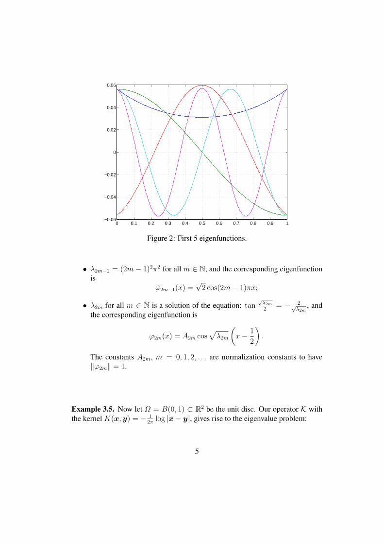
Example 3.5. Now let Ω = B(0, 1) ⊂ R2 be the unit disc. Our operator K withthe kernel K(x, y) = − 1

2πlog |x− y|, gives rise to the eigenvalue problem:

5

−∆ϕ = λϕ , in Ω (DE)∂ϕ∂ν

∣∣∣Γ

= ∂ϕ∂r

∣∣∣Γ

= −∂Hϕ∂θ

∣∣∣Γ, (BC)

where H is the Hilbert transform for the circle:

Hf(θ) , 1

2πpv

∫ π

−π

f(η) cotθ − η

2dη

for all θ ∈ [−π, π]. Now, let βk,` be the `-th zero of the Bessel function of the firstkind of order k, then

ϕm,n(r, θ) =

Jm(βm−1,nr) cos(mθ) for all m,n ∈ NJm(βm−1,nr) sin(mθ) for all m,n ∈ NJ0(β0,nr) if m = 0, n ∈ N

λm,n =

β2

m−1,n if m,n ∈ Nβ2

0,n if m = 0, n ∈ N

(a) (b)

Figure 3: Left: First 25 eigenfunctions of Our integral operator K; Right: First 25eigenfunctions of the Dichlet-Laplace via separation of variables.

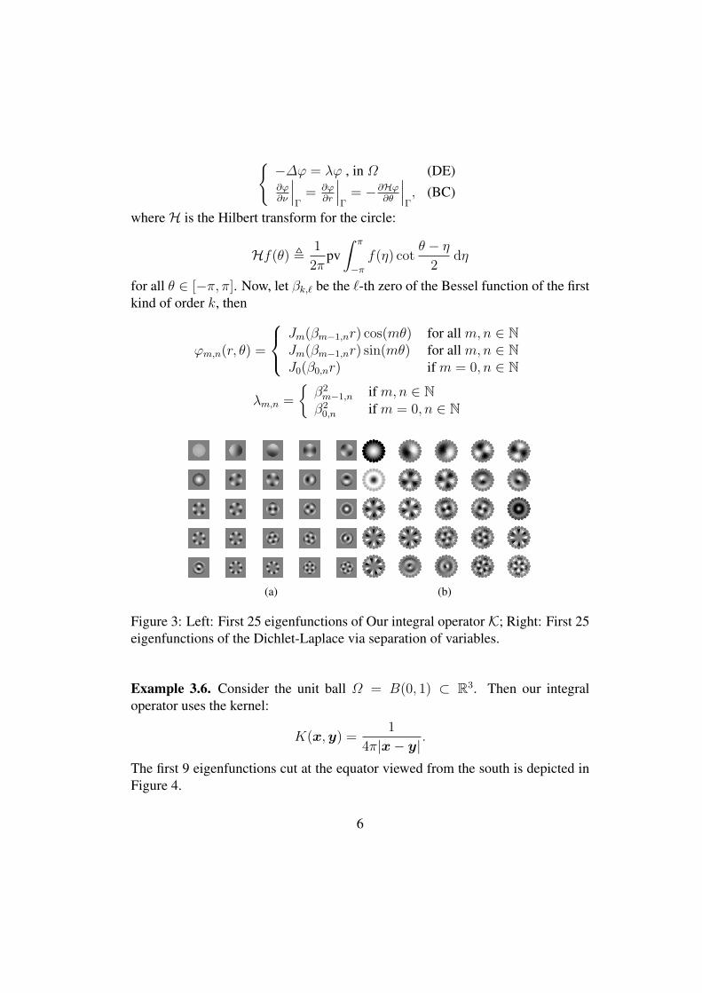
Example 3.6. Consider the unit ball Ω = B(0, 1) ⊂ R3. Then our integraloperator uses the kernel:

K(x, y) =1

4π|x− y| .

The first 9 eigenfunctions cut at the equator viewed from the south is depicted inFigure 4.

6

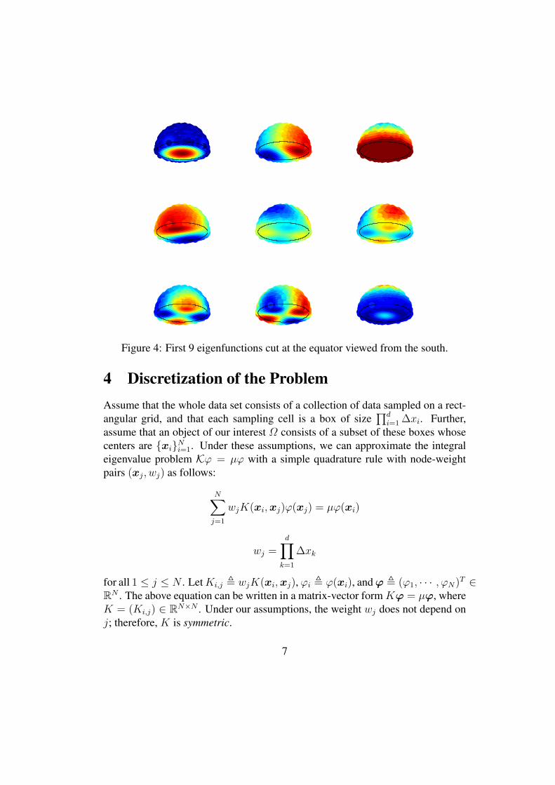
Figure 4: First 9 eigenfunctions cut at the equator viewed from the south.

4 Discretization of the ProblemAssume that the whole data set consists of a collection of data sampled on a rect-angular grid, and that each sampling cell is a box of size

∏di=1 ∆xi. Further,

assume that an object of our interest Ω consists of a subset of these boxes whosecenters are xiN

i=1. Under these assumptions, we can approximate the integraleigenvalue problem Kϕ = µϕ with a simple quadrature rule with node-weightpairs (xj, wj) as follows:

N∑j=1

wjK(xi,xj)ϕ(xj) = µϕ(xi)

wj =d∏

k=1

∆xk

for all 1 ≤ j ≤ N . Let Ki,j , wjK(xi,xj), ϕi , ϕ(xi), and ϕ , (ϕ1, · · · , ϕN)T ∈RN . The above equation can be written in a matrix-vector form Kϕ = µϕ, whereK = (Ki,j) ∈ RN×N . Under our assumptions, the weight wj does not depend onj; therefore, K is symmetric.

7

5 Applications

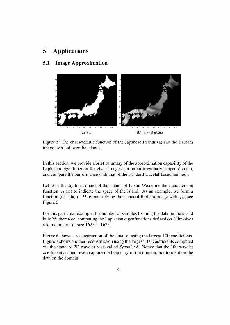
5.1 Image Approximation

10 20 30 40 50 60 70 80 90 100

10

20

30

40

50

60

70

80

90

(a) χΩ

10 20 30 40 50 60 70 80 90 100

10

20

30

40

50

60

70

80

90

(b) χΩ · Barbara

Figure 5: The characteristic function of the Japanese Islands (a) and the Barbaraimage overlaid over the islands.

In this section, we provide a brief summary of the approximation capability of theLaplacian eigenfunction for given image data on an irregularly-shaped domain,and compare the performance with that of the standard wavelet-based methods.

Let Ω be the digitized image of the islands of Japan. We define the characteristicfunction χΩ(x) to indicate the space of the island. As an example, we form afunction (or data) on Ω by multiplying the standard Barbara image with χΩ; seeFigure 5.

For this particular example, the number of samples forming the data on the islandis 1625; therefore, computing the Laplacian eigenfunctions defined on Ω involvesa kernel matrix of size 1625 × 1625.

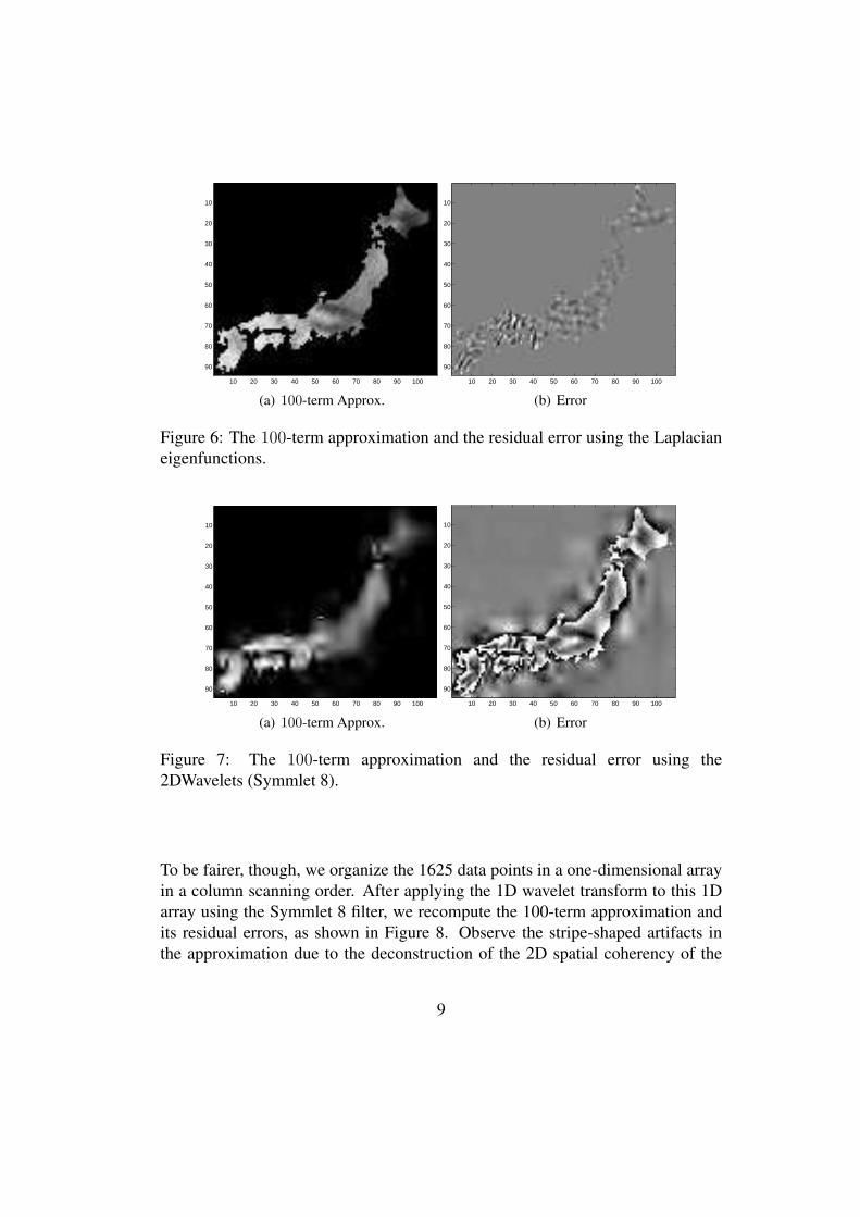
Figure 6 shows a reconstruction of the data set using the largest 100 coefficients.Figure 7 shows another reconstruction using the largest 100 coefficients computedvia the standard 2D wavelet basis called Symmlet 8. Notice that the 100 waveletcoefficients cannot even capture the boundary of the domain, not to mention thedata on the domain.

8

10 20 30 40 50 60 70 80 90 100

10

20

30

40

50

60

70

80

90

(a) 100-term Approx.10 20 30 40 50 60 70 80 90 100

10

20

30

40

50

60

70

80

90

(b) Error

Figure 6: The 100-term approximation and the residual error using the Laplacianeigenfunctions.

10 20 30 40 50 60 70 80 90 100

10

20

30

40

50

60

70

80

90

(a) 100-term Approx.10 20 30 40 50 60 70 80 90 100

10

20

30

40

50

60

70

80

90

(b) Error

Figure 7: The 100-term approximation and the residual error using the2DWavelets (Symmlet 8).

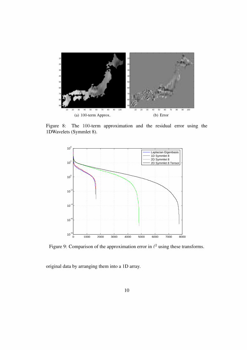
To be fairer, though, we organize the 1625 data points in a one-dimensional arrayin a column scanning order. After applying the 1D wavelet transform to this 1Darray using the Symmlet 8 filter, we recompute the 100-term approximation andits residual errors, as shown in Figure 8. Observe the stripe-shaped artifacts inthe approximation due to the deconstruction of the 2D spatial coherency of the

9

10 20 30 40 50 60 70 80 90 100

10

20

30

40

50

60

70

80

90

(a) 100-term Approx.10 20 30 40 50 60 70 80 90 100

10

20

30

40

50

60

70

80

90

(b) Error

Figure 8: The 100-term approximation and the residual error using the1DWavelets (Symmlet 8).

0 1000 2000 3000 4000 5000 6000 7000 800010

−8

10−6

10−4

10−2

100

102

104

Laplacian Eigenbasis1D Symmlet 82D Symmlet 82D Symmlet 8 Tensor

Figure 9: Comparison of the approximation error in `2 using these transforms.

original data by arranging them into a 1D array.

10

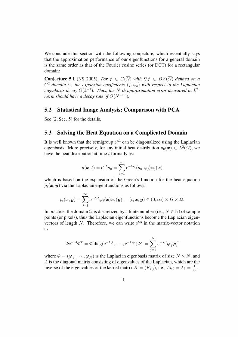
We conclude this section with the following conjecture, which essentially saysthat the approximation performance of our eigenfunctions for a general domainis the same order as that of the Fourier cosine series (or DCT) for a rectangulardomain:

Conjecture 5.1 (NS 2005). For f ∈ C(Ω) with ∇f ∈ BV (Ω) defined on aC2-domain Ω, the expansion coefficients 〈f, ϕk〉 with respect to the Laplacianeigenbasis decay O(k−1). Thus, the N -th approximation error measured in L2-norm should have a decay rate of O(N−1.5).

5.2 Statistical Image Analysis; Comparison with PCASee [2, Sec. 5] for the details.

5.3 Solving the Heat Equation on a Complicated DomainIt is well known that the semigroup et∆ can be diagonalized using the Laplacianeigenbasis. More precisely, for any initial heat distribution u0(x) ∈ L2(Ω), wehave the heat distribution at time t formally as:

u(x, t) = et∆u0 =∞∑

j=1

e−tλj〈u0, ϕj〉ϕj(x)

which is based on the expansion of the Green’s function for the heat equationρt(x, y) via the Laplacian eigenfunctions as follows:

ρt(x,y) =∞∑

j=1

e−λjtϕj(x)ϕj(y), (t, x, y) ∈ (0,∞)×Ω ×Ω.

In practice, the domain Ω is discretized by a finite number (i.e., N ∈ N) of samplepoints (or pixels), thus the Laplacian eigenfunctions become the Laplacian eigen-vectors of length N . Therefore, we can write et∆ in the matrix-vector notationas

Φe−tΛΦT = Φ diag(e−λ1t, · · · , e−λN t)ΦT =N∑

j=1

e−λjtϕjϕTj

where Φ = (ϕ1, · · · ,ϕN) is the Laplacian eigenbasis matrix of size N ×N , andΛ is the diagonal matrix consisting of eigenvalues of the Laplacian, which are theinverse of the eigenvalues of the kernel matrix K = (Ki,j), i.e., Λk,k = λk = 1

µk.

11

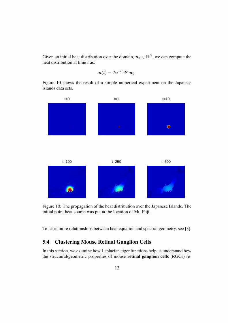
Given an initial heat distribution over the domain, u0 ∈ RN , we can compute theheat distribution at time t as:

u(t) = Φe−tΛΦT u0.

Figure 10 shows the result of a simple numerical experiment on the Japaneseislands data sets.

t=0 t=1 t=10

t=100 t=250 t=500

Figure 10: The propagation of the heat distribution over the Japanese Islands. Theinitial point heat source was put at the location of Mt. Fuji.

To learn more relationships between heat equation and spectral geometry, see [3].

5.4 Clustering Mouse Retinal Ganglion CellsIn this section, we examine how Laplacian eigenfunctions help us understand howthe structural/geometric properties of mouse retinal ganglion cells (RGCs) re-

12

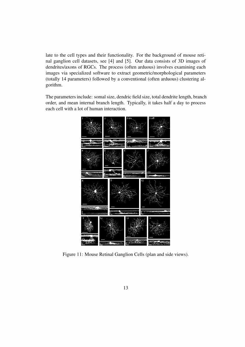
late to the cell types and their functionality. For the background of mouse reti-nal ganglion cell datasets, see [4] and [5]. Our data consists of 3D images ofdendrites/axons of RGCs. The process (often arduous) involves examining eachimages via specialized software to extract geometric/morphological parameters(totally 14 parameters) followed by a conventional (often arduous) clustering al-gorithm.

The parameters include: somal size, dendric field size, total dendrite length, branchorder, and mean internal branch length. Typically, it takes half a day to processeach cell with a lot of human interaction.

Figure 11: Mouse Retinal Ganglion Cells (plan and side views).

13

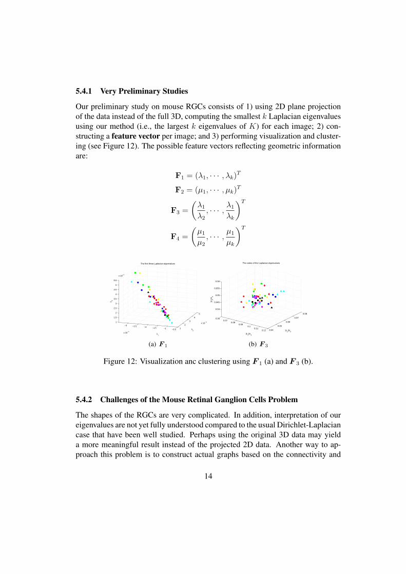
5.4.1 Very Preliminary Studies

Our preliminary study on mouse RGCs consists of 1) using 2D plane projectionof the data instead of the full 3D, computing the smallest k Laplacian eigenvaluesusing our method (i.e., the largest k eigenvalues of K) for each image; 2) con-structing a feature vector per image; and 3) performing visualization and cluster-ing (see Figure 12). The possible feature vectors reflecting geometric informationare:

F1 = (λ1, · · · , λk)T

F2 = (µ1, · · · , µk)T

F3 =

(λ1

λ2

, · · · ,λ1

λk

)T

F4 =

(µ1

µ2

, · · · ,µ1

µk

)T

−3 −2.5 −2 −1.5 −1 −0.5

x 10−4

1

2

3

4

5

x 10−31

1.5

2

2.5

3

3.5

4

4.5

5

5.5

x 10−3

λ2

λ1

The first three Laplacian eigenvalues

λ 3

(a) F 1

0.060.07

0.080.09

0.10.11

0.12 0.04

0.05

0.06

0.07

0.08

0.04

0.045

0.05

0.055

0.06

|λ1|/λ

3

The ratios of the Laplacian eigenvalues

|λ1|/λ

2

|λ1|/λ

4

(b) F 3

Figure 12: Visualization anc clustering using F 1 (a) and F 3 (b).

5.4.2 Challenges of the Mouse Retinal Ganglion Cells Problem

The shapes of the RGCs are very complicated. In addition, interpretation of oureigenvalues are not yet fully understood compared to the usual Dirichlet-Laplaciancase that have been well studied. Perhaps using the original 3D data may yielda more meaningful result instead of the projected 2D data. Another way to ap-proach this problem is to construct actual graphs based on the connectivity and

14

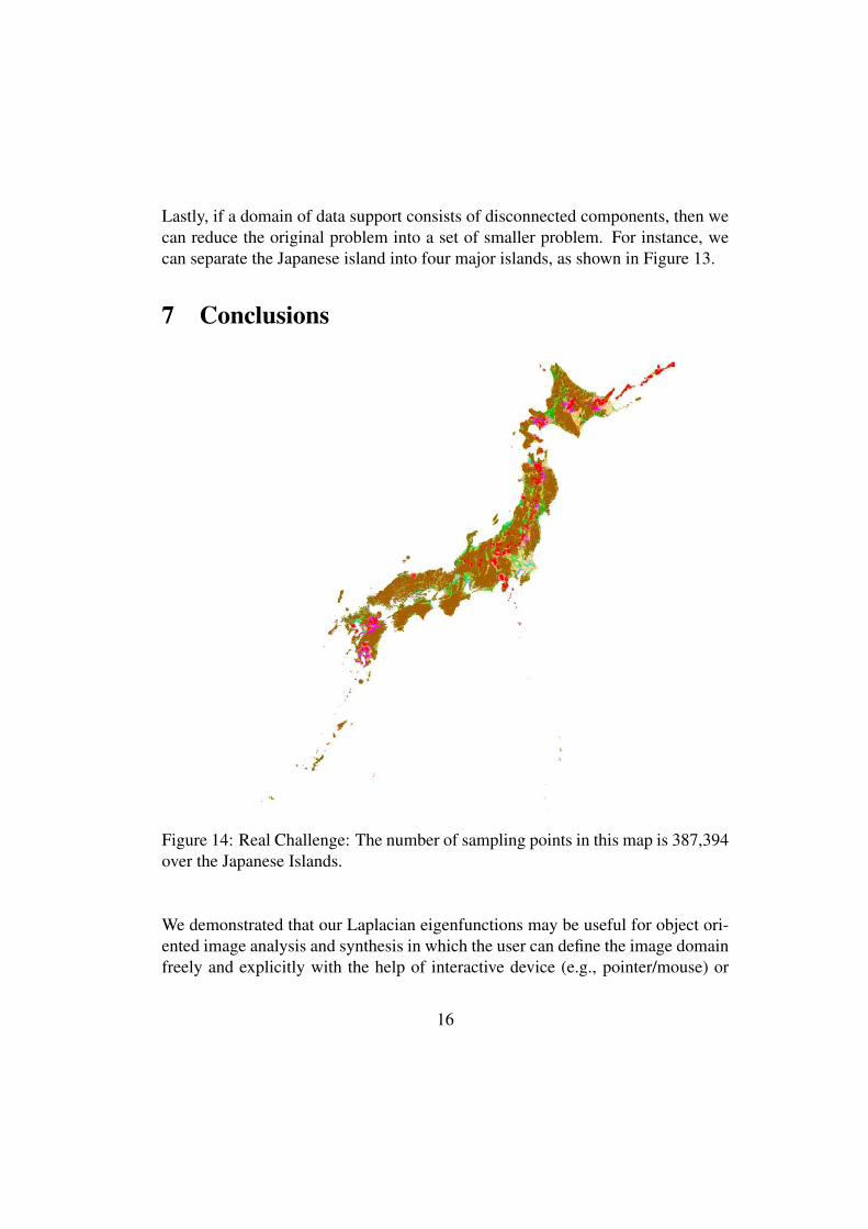
analyze them directly via spectral graph theory and diffusion maps (see Lectures18-20). Lastly, because we are dealing with very complicated domains with manysample points (see Figure 14), we need to develop a faster algorithm to reducecomputational burden.

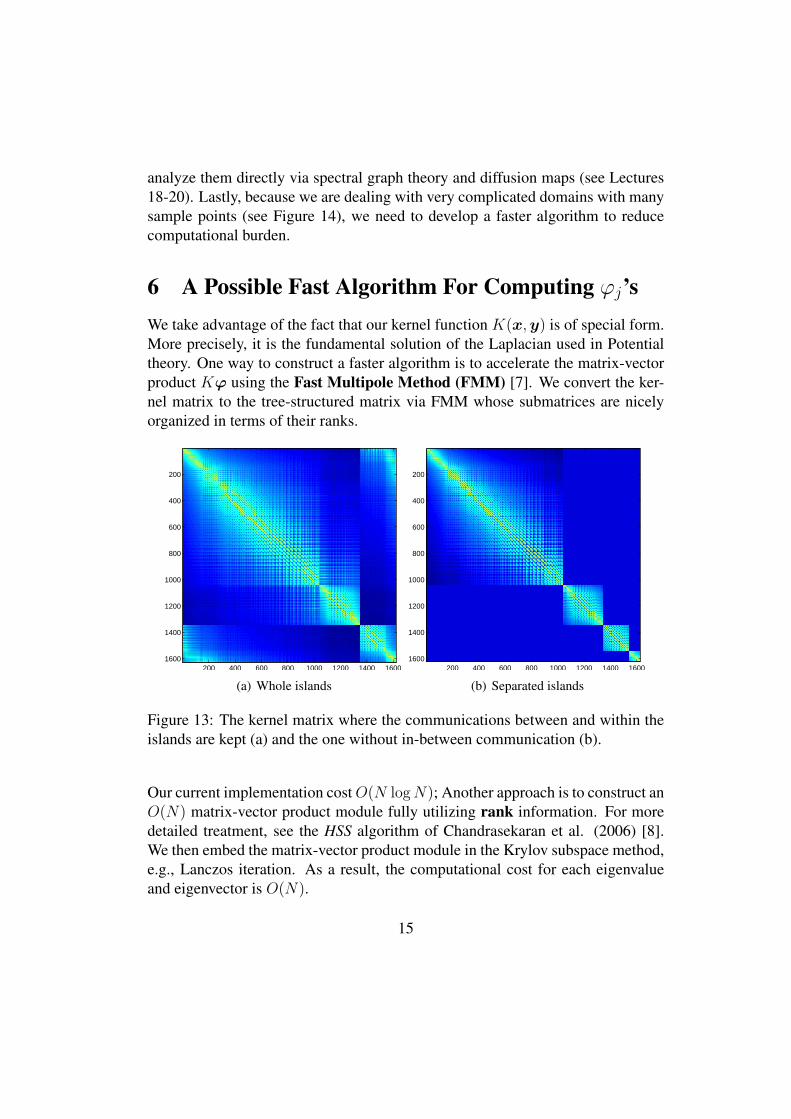
6 A Possible Fast Algorithm For Computing ϕj’sWe take advantage of the fact that our kernel function K(x,y) is of special form.More precisely, it is the fundamental solution of the Laplacian used in Potentialtheory. One way to construct a faster algorithm is to accelerate the matrix-vectorproduct Kϕ using the Fast Multipole Method (FMM) [7]. We convert the ker-nel matrix to the tree-structured matrix via FMM whose submatrices are nicelyorganized in terms of their ranks.

200 400 600 800 1000 1200 1400 1600

200

400

600

800

1000

1200

1400

1600

(a) Whole islands200 400 600 800 1000 1200 1400 1600

200

400

600

800

1000

1200

1400

1600

(b) Separated islands

Figure 13: The kernel matrix where the communications between and within theislands are kept (a) and the one without in-between communication (b).

Our current implementation cost O(N log N); Another approach is to construct anO(N) matrix-vector product module fully utilizing rank information. For moredetailed treatment, see the HSS algorithm of Chandrasekaran et al. (2006) [8].We then embed the matrix-vector product module in the Krylov subspace method,e.g., Lanczos iteration. As a result, the computational cost for each eigenvalueand eigenvector is O(N).

15

Lastly, if a domain of data support consists of disconnected components, then wecan reduce the original problem into a set of smaller problem. For instance, wecan separate the Japanese island into four major islands, as shown in Figure 13.

7 Conclusions

Figure 14: Real Challenge: The number of sampling points in this map is 387,394over the Japanese Islands.

We demonstrated that our Laplacian eigenfunctions may be useful for object ori-ented image analysis and synthesis in which the user can define the image domainfreely and explicitly with the help of interactive device (e.g., pointer/mouse) or

16

some automatic segmentation algorithm. We also demonstrated that our methodbased on the eigenanalysis of the commuting integral operator leads to uncon-ventional non-local boundary condition for the Laplacian eigenvalue problem, butthat the numerical implementation is straightforward and is amenable to modernfast algorithms. Our experiments and analogy with the analytic examples suggestthat we should be able to get fast-decaying expansion coefficients if the imagesare in C(Ω) and ∇f ∈ BV(Ω), where the boundary of Ω is smooth. In essence,our method can be viewed as a replacement of DCT for the general shape domain.This means that our eigenfunctions have a variety of potential applications e.g.,interpolation, extrapolation, local feature computation, and perhaps compression.In addition, it connects several interesting mathematics, including spectral geom-etry, spectral graph theory, isoperimetric inequalities, Toeplitz operators, PDEs,potential theory, and almost-periodic functions.

References[1] N. SAITO, “Geometric Harmonics as a Statistical Image Processing Tool for

Images Defined on Irregularly Shaped Domains,” in Proc. IEEE Workshopon Statistical Image Processing, Bordeaux, France, Jul. 2005

[2] N. SAITO, “Data Analysis and Representation Using Eigenfunctions ofLaplacians on a General Domain,” Submitted to Applied and ComputationalHarmonic Analysis, Mar. 2007

[3] J. DODZIUK, ”Eigenvalues of the Laplacian and the Heat Equation,” Amer.Math. Monthly, vol. 88, no. 9, pp. 686-695, 1981.

[4] J, COOMBS, D. VAN DER LIST, G.-Y. WANG, AND L.M. CHALUPA, “Mor-phological Properties of Mouse Retinal Ganglion Cells”, Neuroscience, vol.140, no. 1, pp. 123-136, 2006.

[5] J.-H. KONG, D.R. FISH, R.L. ROCKHILL, AND R.H. MASLAND, “Di-versity of Ganglion Cells in the Mouse Retina: Unsupervised Morpholog-ical Classification and its Limits”, The Journal of Comparative Neurology,vol. 489, no. 3, pp. 293-310, 2005.

[6] A. CANTONI, P. BUTLER, “Eigenvalues and eigenvectors of symmetric cen-trosymmetric matrices”, Linear Algebra Appl., vol. 13, pp. 275-288, 1976.

17

[7] L. GREENGARD, V. ROKHLIN, “A fast algorithm for particle simulations”,J. Comput. Phys., vol. 73, pp. 325-348, 1987.

[8] S. CHANDRASEKARAN, M. GU, AND T. PALS, “A fast ULV decompositionsolver for hierarchically semi-separable representations”, SIAM J. MatrixAnal. Appl., vol. 28, No. 3, pp. 603C622, 2006.

18