Littlest Seesaw

Stephen F. King∗,Physics and Astronomy, University of Southampton, Southampton, SO17 1BJ, U.K.

Abstract

We propose the Littlest Seesaw (LS) model consisting of just two right-handedneutrinos, where one of them, dominantly responsible for the atmospheric neutrinomass, has couplings to (νe, νµ, ντ ) proportional to (0, 1, 1), while the subdominant right-handed neutrino, mainly responsible for the solar neutrino mass, has couplings to(νe, νµ, ντ ) proportional to (1, n, n− 2). This constrained sequential dominance (CSD)model preserves the first column of the tri-bimaximal (TB) mixing matrix (TM1) and

has a reactor angle θ13 ∼ (n − 1)√

23m2m3

. This is a generalisation of CSD (n = 1)which led to TB mixing and arises almost as easily if n ≥ 1 is a real number. Wederive exact analytic formulas for the neutrino masses, lepton mixing angles and CPphases in terms of the four input parameters and discuss exact sum rules. We showhow CSD (n = 3) may arise from vacuum alignment due to residual symmetries ofS4. We propose a benchmark model based on S4 × Z3 × Z ′3, which fixes n = 3 andthe leptogenesis phase η = 2π/3, leaving only two inputs ma and mb = mee describing∆m2

31, ∆m221 and UPMNS . The LS model predicts a normal mass hierarchy with a

massless neutrino m1 = 0 and TM1 atmospheric sum rules. The benchmark LS modeladditionally predicts: solar angle θ12 = 34◦, reactor angle θ13 = 8.7◦, atmosphericangle θ23 = 46◦, and Dirac phase δCP = −87◦.

1 Introduction

The discovery of neutrino oscillations, implying mass and mixing, remains one of the greatestdiscoveries in physics in the last two decades. Although the origin of neutrino mass ispresently unknown (for reviews see e.g.[1]), whatever is responsible must be new physicsbeyond the Standard Model (BSM). For example, the leading candidate for neutrino mass

∗king@soton.ac.uk

1

arX

iv:1

512.

0753

1v2

[he

p-ph

] 1

Mar

201

6

and mixing is the seesaw mechanism involving additional right-handed neutrinos with heavyMajorana masses [2], providing an elegant explanation of the smallness of neutrino mass 1.

However, in general, the seesaw mechanism typically involves many parameters, makingquantitative predictions of neutrino mass and mixing challenging. In this respect, the seesawmechanism offers no more understanding of flavour than the Yukawa couplings of the SM.Indeed it introduces a new flavour sector associated with right-handed neutrino Majoranamasses, which cannot be directly probed by high energy particle physics experiment. Clearlya different approach is required to make progress with the new (or nu) Standard Model thatinvolves the seesaw mechanism. Here we shall make use of the theoretical touchstones ofelegance and simplicity (which indeed motivate the seesaw mechanism in the first place) totry to allow some experimental guidance to inform the high energy seesaw mechanism. If theassumptions we make prove to be inconsistent with experiment then we must think again,otherwise the framework of assumptions remains viable.

In this paper, then, we focus on natural implementations of the seesaw mechanism, wheretypically one of the right-handed neutrinos is dominantly responsible for the atmosphericneutrino mass [4], while a second subdominant right-handed neutrino accounts for the solarneutrino mass [5]. This idea of sequential dominance (SD) of right-handed neutrinos is anelegant hypothesis which, when combined with the assumption of a zero coupling of theatmospheric neutrino to νe, leads to the generic bound θ13

<∼ m2/m3 [6], which appears tobe approximately saturated according to current measurements of the reactor angle. Thisbound was derived over a decade before the experimental measurement of the reactor angle.This success supports the SD approach, and motivates efforts to understand why the reactorbound is approximately saturated. In order to do this one needs to further constrain theYukawa couplings beyond the assumption of a single texture zero as assumed above.

The idea of constrained sequential dominance (CSD) is that the “atmospheric” right-handedneutrino has couplings to (νe, νµ, ντ ) proportional to (0, 1, 1), while the “solar” right-handedneutrino has couplings to (νe, νµ, ντ ) proportional to (1, n, n−2) where n is a real number. Itturns out that such a structure preserves the first column of the tri-bimaximal (TB) [7] mixing

matrix (TM1), leading to the approximate result θ13 ∼ (n − 1)√

23m2

m3, which we shall derive

here from exact results. This scheme is therefore a generalisation of the original CSD(n = 1)[8] which led to TB mixing and the prediction θ13 = 0, which is now excluded. It is also

a generalisation of CSD(n = 2) [9] which predicted θ13 ∼√

23m2

m3, which was subsequently

proved to be too small when more precise measurements of θ13 were made. It seems we arethird time lucky since CSD(n = 3) [10] predicts θ13 ∼ 2

√2

3m2

m3which is in broad agreement

with current measurements. On the other hand CSD(n = 4) [11, 12] predicts θ13 ∼√

2m2

m3

appears to be a little too large, unless a third right-handed neutrino is invoked (unavoidablein Pati-Salam for example [13]), while CSD(n ≥ 5) [14] is excluded. Recently, CSD(3) hasbeen exploited in Grand Unified Theories (GUTs) based on SU(5) [15,16] and SO(10) [17].

1For a simple introduction to the seesaw mechanism see e.g.[3].

2

The new approach and results in this paper are summarised below:

• The approach here is more general than previously considered, since we allow n tobe a real number, rather than being restricted to the field of positive integers. Themotivation is that the vacuum alignment vector (1, n, n− 2) is orthogonal to the firstcolumn of the TB matrix (2,−1, 1) (which in turn is orthogonal to the second and thirdTB columns (1, 1,−1) and (0, 1, 1)) for any real number n, emerges very naturally asdepicted in Fig.1. This provides a plausible motivation for considering the vacuumalignment direction (1, n, n − 2) for any real number n. We refer to the associatedminimal models as the Littlest Seesaw (LS). The LS with CSD(n) predicts a normalmass hierarchy with a massless neutrino m1 = 0, both testable in the near future.Actually the above predictions also arise in general two right-handed neutrino models.What distinguishes the LS model from general two right-handed neutrino models arethe predictions for the lepton mixing angles and CP phases as discussed below.

• For the general case of any real value of n ≥ 1, for the first time we shall derive exactanalytic formulas for the neutrino masses, lepton mixing angles and CP phases (bothDirac and Majorana) in terms of the four input parameters. This is progress sincepreviously only numerical results were used. We also show that CSD(n) is subjectto the TM1 mixing sum rules and no other ones. From the exact results, which areuseful for many purposes but a little lengthy, we extract some simple approximationswhich provide some rough and ready insight into what is going on. For example,the approximate result θ13 ∼ (n− 1)

√2

3m2

m3provides an analytic understanding of why

CSD(n ≥ 5) is excluded, which until now has only been a numerical finding.

• We show that the successful case of CSD(3) arises more naturally from symmetry in thecase of S4, rather than using A4, as was done in previous work [10–15]. The reason isthat both the neutrino scalar vacuum alignments (0, 1, 1) and (1, 3, 1) preserve residualsubgroups of S4 which are not present in A4. This motivates models based on S4,extending the idea of residual symmetries from the confines of two sectors (the chargedlepton and neutrino sectors) as is traditionally done in direct models, to five sectors,two associated with the neutrinos and three with the charged leptons, as summarisedin the starfish shaped diagram in Fig.2.

• Finally we present a benchmark LS model based on S4×Z3×Z ′3, with supersymmetricvacuum alignment, which not only fixes n = 3 but also the leptogenesis phase η = 2π/3,leaving only two continuous input masses, yielding two neutrino mass squared splittingsand the PMNS matrix. A single Z3 factor is required to understand η = 2π/3 as acube root of unity, while an additional Z ′3 is necessary to understand the charged leptonmass hierarchy and also to help to control the operator structure of the model. Themodel provides a simple LS framework for the numerical benchmark predictions: solarangle θ12 = 34◦, reactor angle θ13 = 8.7◦, atmospheric angle θ23 = 46◦, and Dirac phaseδCP = −87◦, which are readily testable in forthcoming oscillation experiments.

3

The layout of the remainder of the paper is as follows. In section 2 we briefly introduce thetwo right-handed neutrino model and motivate CSD(n). In section 3 we show how CSD(n)implies TM1 mixing. In section 4 we briefly review the direct and indirect approaches tomodel building, based on flavour symmetry. In section 5 we pursue the indirect approachand show how vacuum alignment for CSD(n) can readily be obtained from the TB vacuumalignments using orthogonality. In section 6 we write down the Lagrangian of the LS modeland derive the neutrino mass matrix from the seesaw mechanism with CSD(n). In section 7we discuss a numerical benchmark, namely CSD(3) with leptogenesis phase η = 2π/3 and itsconnection with the oscillation phase. In sections 8, 9, 10 we derive exact analytic formulasfor the angles, masses and CP phases, for the LS model with general CSD(n) valid for realn ≥ 1, in terms of the four input parameters of the model. In section 11 present the exactTM1 atmospheric sum rules, which we argue are the only ones satisfied by the model. Insection 12 we focus on the reactor and atmospheric angles and, starting from the exactresults, derive useful approximate formulae which can provide useful insight. In section 13we show how vacuum alignment for CSD(3) can arise from the residual symmetries of S4, assummarised by the starfish diagram in Fig.2. In sections 14 and 15 we present a benchmarkLS model based on the discrete group S4×Z3×Z ′3, with supersymmetric vacuum alignment,which not only fixes n = 3 but also the leptogenesis phase η = 2π/3, reproducing theparameters of the numerical benchmark. Section 16 concludes the paper. There are twoappendices, Appendix A on lepton mixing conventions and Appendix B on S4.

2 Seesaw mechanism with two right-handed neutrinos

The two right-handed neutrino seesaw model was first proposed in [5]. Subsequently tworight-handed neutrino models with two texture zeros were discussed in [18], however suchtwo texture zero models are now phenomenologically excluded [19] for the case of a normalneutrino mass hierarchy considered here. However the two right-handed neutrino model withone texture zero (actually also suggested in [5]), remains viable.

With two right-handed neutrinos, the Dirac mass matrix mD is, in LR convention,

mD =

d ae bf c

, (mD)T =

(d e fa b c

)(1)

The (diagonal) right-handed neutrino heavy Majorana mass matrixMR with rows (νatmR , νsol

R )T

and columns (νatmR , νsol

R ) is,

MR =

(Matm 0

0 Msol

), M−1

R =

(M−1

atm 00 M−1

sol

)(2)

4

The light effective left-handed Majorana neutrino mass matrix is given by the seesaw formula

mν = −mDM−1R mDT , (3)

Using the see-saw formula dropping the overall minus sign which is physically irrelevant, wefind, by multiplying the matrices in Eqs.1,2,

mν = mDM−1R (mD)T =

a2

Msol+ d2

Matm

abMsol

+ deMatm

acMsol

+ dfMatm

abMsol

+ deMatm

b2

Msol+ e2

Matm

bcMsol

+ efMatm

acMsol

+ dfMatm

bcMsol

+ efMatm

c2

Msol+ f2

Matm

(4)

Motivated by the desire to implement the seesaw mechanism in a natural way, sequentialdominance (SD) [4, 5] assumes that the two right-handed neutrinos νsol

R and νatmR have cou-

plings d� e, f and(e, f)2

Matm

� (a, b, c)2

Msol

. (5)

By explicit calculation, using Eq.4, one can check that in the two right-handed neutrino limitdetmν = 0. Since the determinant of a Hermitian matrix is the product of mass eigenvalues

det(mνmν†) = m21m

22m

23,

one may deduce that one of the mass eigenvalues of the complex symmetric matrix aboveis zero, which under the SD assumption is the lightest one m1 = 0 with m3 � m2 sincethe model approximates to a single right-handed neutrino model [4]. Hence we see that SDimplies a normal neutrino mass hierarchy. Including the solar right-handed neutrino as aperturbation, it can be shown that, for d = 0, together with the assumption of a dominantatmospheric right-handed neutrino in Eq.5, leads to the approximate results for the solarand atmospheric angles [4, 5],

tan θ23 ∼e

f, tan θ12 ∼

√2a

b− c. (6)

Under the above SD assumption, each of the right-handed neutrinos contributes uniquelyto a particular physical neutrino mass. The SD framework above with d = 0 leads to therelations in Eq.6 together with the reactor angle bound [6],

θ13 .m2

m3

(7)

This result shows that SD allows for large values of the reactor angle, consistent with themeasured value. Indeed the measured reactor angle, observed a decade after this theoreticalbound was derived, approximately saturates the upper limit. In order to understand whythis is so, we must go beyond the SD assumptions stated so far.

5

Motivated by the desire to obtain an approximately maximal atmospheric angle tan θ23 ∼ 1and trimaximal solar angle tan θ12 ∼ 1/

√2, the results in Eq.6 suggest constraining the

Dirac matrix elements in Eq.1 to take the values d = 0 with e = f and b = na and alsoc = (n− 2)a,

mD =

0 ae nae (n− 2)a

, (8)

which, for any positive integer n, is referred to as constrained sequential dominance (CSD)[8–14]. In section 12 we shall show that Eq.8 also implies,

θ13 ∼ (n− 1)

√2

3

m2

m3

, (9)

so that the bound in Eq.7 is approximately saturated for n ∼ 3.

As already mentioned, we refer to a two right-handed neutrino model in which the Diracmass matrix in the flavour basis satisfies Eq.8, with n being a real number, as the “LittlestSeesaw” or LS model. The justification for this terminology is that it represents the seesawmodel with the fewest number of parameters consistent with current neutrino data. To beprecise, in the flavour basis, the Dirac mass matrix of the LS model involves two complexparameters e, a plus one real parameter n. This is fewer than the original two right-handedneutrino Dirac mass matrix which involves six complex parameters [5]. It is also fewer thanthe two right-handed neutrino model in [6] which involves five complex parameters due tothe single texture zero. It is even fewer than the minimal right-handed neutrino model in[18] which involves four complex parameters due to the two texture zeroes. It remains tojustify the Dirac structure of the LS model in Eq.8, and we shall address this question usingsymmetry and vacuum alignment in subsequent sections.

3 Trimaximal Mixing

A simple example of lepton mixing which came to dominate the model building communityuntil the measurement of the reactor angle is the tribimaximal (TB) mixing matrix [7]. Itpredicts zero reactor angle θ13 = 0, maximal atmospheric angle s2

23 = 1/2, or θ12 = 45◦, anda solar mixing angle given by s12 = 1/

√3, i.e. θ12 ≈ 35.3◦. The mixing matrix is given

explicitly by

UTB =

√23

1√3

0

− 1√6

1√3

1√2

1√6− 1√

31√2

. (10)

Unfortunately TB mixing is excluded since it predicts a zero reactor angle. However CSDin Eq.8 with two right-handed neutrinos allows a non-zero reactor angle for n > 1 and also

6

predicts the lightest physical neutrino mass to be zero, m1 = 0. One can also check that theneutrino mass matrix resulting from using Eq.8 in the seesaw formula in Eq.3, satisfies

mν

2−11

=

000

. (11)

In other words the column vector (2,−1, 1)T is an eigenvector of mν with a zero eigenvalue,i.e. it is the first column of the PMNS mixing matrix, corresponding to m1 = 0, which meansso called TM1 mixing [20,21] in which the first column of the TB mixing matrix in Eq.10 ispreserved, while the other two columns are allowed to differ (in particular the reactor anglewill be non-zero for n > 1),

UTM1 =

√23− −

− 1√6− −

1√6− −

. (12)

Interestingly CSD in Eq.8 with n = 1 [8] predicts a zero reactor angle and hence TB mixing,while for n > 1 it simply predicts the less restrictive TM1 mixing. Having seen that CSDleads to TB, or more generally TM1 mixing, we now discuss the theoretical origin of thedesired Dirac mass matrix structure in Eq.8.

4 Flavour symmetry: direct versus indirect models

Let us expand the neutrino mass matrix in the diagonal charged lepton basis, assuming exactTB mixing, as mν

TB = UTBdiag(m1,m2,m3)UTTB leading to (absorbing the Majorana phases

in mi):mνTB = m1Φ1ΦT

1 +m2Φ2ΦT2 +m3Φ3ΦT

3 (13)

where

ΦT1 =

1√6

(2,−1, 1), ΦT2 =

1√3

(1, 1,−1), ΦT3 =

1√2

(0, 1, 1), (14)

are the respective columns of UTB and mi are the physical neutrino masses. In the neutrinoflavour basis (i.e. diagonal charged lepton mass basis), it has been shown that the above TBneutrino mass matrix is invariant under S, U transformations:

mνTB = Smν

TBST = Umν

TBUT . (15)

A very straightforward argument [22] shows that this neutrino flavour symmetry group hasonly four elements corresponding to Klein’s four-group ZS

2 × ZU2 . By contrast the diagonal

charged lepton mass matrix (in this basis) satisfies a diagonal phase symmetry T . In thecase of TB mixing, the matrices S, T, U form the generators of the group S4 in the tripletrepresentation, while the A4 subgroup is generated by S, T .

7

As discussed in [22], the flavour symmetry of the neutrino mass matrix may originate fromtwo quite distinct classes of models. The class of models, which we call direct models, arebased on a family symmetry such as S4, for example, where the symmetry of the neutrinomass matrix is a remnant of the S4 symmetry of the Lagrangian, with the generators S, Upreserved in the neutrino sector, while the diagonal generator T is preserved in the chargedlepton sector. If U is broken but S is preserved, then this leads to TM2 mixing with thesecond column of the TB mixing matrix being preserved. However if the combination SUis preserved then this corresponds to TM1 mixing with the first column of the TB mixingmatrix being preserved [23]. Of course, the S4 symmetry is completely broken in the fulllepton Lagrangian including both neutrino and charged lepton sectors.

In an alternative class of models, which we call indirect models, the family symmetry isalready completely broken in the neutrino sector, where the observed neutrino flavour sym-metry ZS

2 × ZU2 emerges as an accidental symmetry. However the structure of the Dirac

mass matrix is controlled by vacuum alignment in the flavour symmetry breaking sector, asdiscussed in the next section. The indirect models are arguably more natural than the directmodels, especially for m1 = 0, since each column of the Dirac mass matrix corresponds toa different symmetry breaking VEV and each contribution to the seesaw mechanism cor-responds to a different right-handed neutrino mass, enabling mass hierarchies to naturallyemerge. Thus a strong mass hierarchy m1 � m2 < m3 would seem to favour indirect modelsover direct models, so we pursue this possibility in the following.

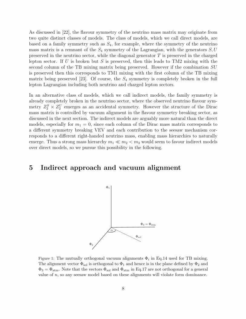
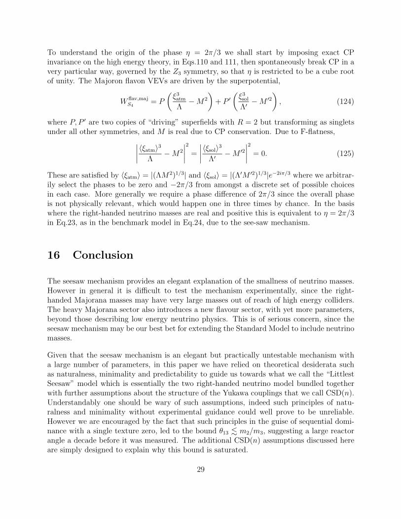
5 Indirect approach and vacuum alignment

�1

�2

�sol

�3 = �atm

↵

Figure 1: The mutually orthogonal vacuum alignments Φi in Eq.14 used for TB mixing.The alignment vector Φsol is orthogonal to Φ1 and hence is in the plane defined by Φ2 andΦ3 = Φatm. Note that the vectors Φsol and Φatm in Eq.17 are not orthogonal for a generalvalue of n, so any seesaw model based on these alignments will violate form dominance.

8

The basic idea of the indirect approach is to effectively promote the columns of the Diracmass matrix to fields which transform as triplets under the flavour symmetry. We assumethat the Dirac mass matrix can be written as mD = (aΦatm, bΦsol, cΦdec) where the columnsare proportional to triplet Higgs scalar fields with particular vacuum alignments and a, b, care three constants of proportionality. Working in the diagonal right-handed neutrino massbasis, the seesaw formula gives,

mν = a2 ΦatmΦTatm

Matm

+ b2 ΦsolΦTsol

Msol

+ c2 ΦdecΦTdec

Mdec

, (16)

By comparing Eq.16 to the TB form in Eq.13 it is clear that TB mixing will be achieved ifΦatm ∝ Φ3 and Φsol ∝ Φ2 and Φdec ∝ Φ1, with each of m3,2,1 originating from a particularright-handed neutrino. The case where the columns of the Dirac mass matrix are proportionalto the columns of the PMNS matrix, the columns being therefore mutually orthogonal, isreferred to as form dominance (FD) [24]. The resulting mν is form diagonalizable. Eachcolumn of the Dirac mass matrix arises from a separate flavon VEV, so the mechanism isvery natural, especially for the case of a strong mass hierarchy. Note that for m1 � m2 < m3

the precise form of Φdec becomes irrelevant and for m1 = 0 we can simply drop the last termand the model reduces to a two right-handed neutrino model.

Within this framework, the general CSD Dirac mass matrix structure in Eq.8 correspondsto there being some Higgs triplets which can be aligned in the directions,

ΦTatm ∝ (0, 1, 1), ΦT

sol ∝ (1, n, n− 2), (17)

The first vacuum alignment Φatm in Eq.17 is just the TB direction ΦT3 in Eq.14. The second

vacuum alignment Φsol in Eq.17 can be easily obtained since the direction (1, n, n − 2) isorthogonal to the TB vacuum alignment ΦT

1 in Eq.14.

For example, in a supersymmetric theory, the aligning superpotential should contain thefollowing terms, enforced by suitable discrete Zn symmetries,

Oijφiφj +Osolφsolφ1 (18)

where the terms proportional to the singlets Oij and Osol ensure that the real S4 tripletsare aligned in mutually orthogonal directions, Φi ⊥ Φj and Φsol ⊥ Φ1 as depicted in Fig. 1.From Eqs.14,17 we can write Φsol = Φ2 cosα + Φ3 sinα where tanα = 2(n − 1)/3 and α isthe angle between Φsol and Φ2, as shown in Fig. 1. Φsol is parallel to Φ2 for n = 1, while itincreasingly tends towards the Φ3 = Φatm alignment as n is increased.

6 The Littlest Seesaw

The littlest seesaw (LS) model consists of the three families of electroweak lepton doubletsL unified into a single triplet of the flavour symmetry, while the two right-handed neutrinos

9

νatmR and νsol

R are singlets. The LS Lagrangian in the neutrino sector takes the form,

L = −yatmL̄.φatmνatmR − ysolL̄.φsolν

solR −

1

2Matmν̄cR

atmνatmR − 1

2Msolν̄cR

solνsolR +H.c. . (19)

which may be enforced by suitable discrete Z3 symmetries, as discussed in section 14. Hereφsol and φatm may be interpreted as either Higgs fields, which transform as triplets of theflavour symmetry with the alignments in Eq.17, or as combinations of a single Higgs elec-troweak doublet together with triplet flavons with these vacuum alignments. Note that, inEq.19, φsol and φatm represent fields, whereas in Eq.17 Φsol and Φatm refer to the VEVs ofthose fields.

In the diagonal charged lepton and right-handed neutrino mass basis, when the fields Φsol

and Φatm in Eq.19 are replaced by their VEVs in Eq.17, this reproduces the Dirac massmatrix in Eq.8 [10] and its transpose:

mD =

0 ae nae (n− 2)a

, mDT =

(0 e ea na (n− 2)a

), (20)

which defines the LS model, where we regard n as a real continuous parameter, later arguingthat it may take simple integer values. The (diagonal) right-handed neutrino heavy Majorana

mass matrix MR with rows (ν̄cRatm, ν̄cR

sol)T and columns (νatm

R , νsolR ) is,

MR =

(Matm 0

0 Msol

), M−1

R =

(M−1

atm 00 M−1

sol

)(21)

The low energy effective Majorana neutrino mass matrix is given by the seesaw formula

mν = −mDM−1R mDT , (22)

which, after multiplying the matrices in Eqs.20, 21, for a suitable choice of physically irrele-vant overall phase, gives

mν = ma

0 0 00 1 10 1 1

+mbe

iη

1 n (n− 2)n n2 n(n− 2)

(n− 2) n(n− 2) (n− 2)2

, (23)

where η is the only physically important phase, which depends on the relative phase between

the first and second column of the Dirac mass matrix, arg(a/e) andma = |e|2Matm

andmb = |a|2Msol

.

This can be thought of as the minimal (two right-handed neutrino) predictive seesaw modelsince only four real parameters ma,mb, n, η describe the entire neutrino sector (three neutrinomasses as well as the PMNS matrix, in the diagonal charged lepton mass basis). As we shallsee in the next section, η is identified with the leptogenesis phase, while mb is identified withthe neutrinoless double beta decay parameter mee.

10

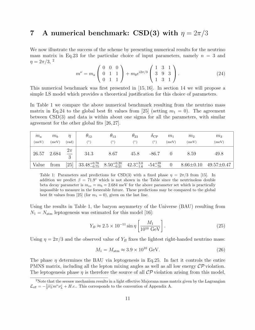
7 A numerical benchmark: CSD(3) with η = 2π/3

We now illustrate the success of the scheme by presenting numerical results for the neutrinomass matrix in Eq.23 for the particular choice of input parameters, namely n = 3 andη = 2π/3, 2

mν = ma

0 0 00 1 10 1 1

+mbe

i2π/3

1 3 13 9 31 3 1

. (24)

This numerical benchmark was first presented in [15, 16]. In section 14 we will propose asimple LS model which provides a theoretical justification for this choice of parameters.

In Table 1 we compare the above numerical benchmark resulting from the neutrino massmatrix in Eq.24 to the global best fit values from [25] (setting m1 = 0). The agreementbetween CSD(3) and data is within about one sigma for all the parameters, with similaragreement for the other global fits [26, 27].

ma

(meV)

mb

(meV)

η(rad)

θ12

(◦)

θ13

(◦)

θ23

(◦)

δCP

(◦)

m1

(meV)

m2

(meV)

m3

(meV)

26.57 2.6842π

334.3 8.67 45.8 -86.7 0 8.59 49.8

Value from [25] 33.48+0.78−0.75 8.50+0.20

−0.21 42.3+3.0−1.6 -54+39

−70 0 8.66±0.10 49.57±0.47

Table 1: Parameters and predictions for CSD(3) with a fixed phase η = 2π/3 from [15]. Inaddition we predict β = 71.9◦ which is not shown in the Table since the neutrinoless doublebeta decay parameter is mee = mb = 2.684 meV for the above parameter set which is practicallyimpossible to measure in the forseeable future. These predictions may be compared to the globalbest fit values from [25] (for m1 = 0), given on the last line.

Using the results in Table 1, the baryon asymmetry of the Universe (BAU) resulting fromN1 = Natm leptogenesis was estimated for this model [16]:

YB ≈ 2.5× 10−11 sin η

[M1

1010 GeV

]. (25)

Using η = 2π/3 and the observed value of YB fixes the lightest right-handed neutrino mass:

M1 = Matm ≈ 3.9× 1010 GeV. (26)

The phase η determines the BAU via leptogenesis in Eq.25. In fact it controls the entirePMNS matrix, including all the lepton mixing angles as well as all low energy CP violation.The leptogenesis phase η is therefore the source of all CP violation arising from this model,

2Note that the seesaw mechanism results in a light effective Majorana mass matrix given by the LagrangianLeff = − 1

2νLmννcL +H.c.. This corresponds to the convention of Appendix A.

11

including CP violation in neutrino oscillations and in leptogenesis. There is a direct linkbetween measurable and cosmological CP violation in this model and a correlation betweenthe sign of the BAU and the sign of low energy leptonic CP violation. The leptogenesis phaseis fixed to be η = 2π/3 which leads to the observed excess of matter over antimatter forM1 ≈ 4.1010 GeV, yielding an observable neutrino oscillation phase δCP ≈ −π/2.

8 Exact analytic results for lepton mixing angles

We would like to understand the numerical success of the neutrino mass matrix analytically.In the following sections we shall derive exact analytic results for neutrino masses and PMNSparameters, for real continuous n, corresponding to the physical (light effective left-handedMajorana) neutrino mass matrix, in the diagonal charged lepton mass basis in Eq.23, whichwe reproduce below,

mν = ma

0 0 00 1 10 1 1

+mbe

iη

1 n n− 2n n2 n(n− 2)1 n(n− 2) (n− 2)2

. (27)

Since this yields TM1 mixing as discussed above, it can be block diagonalised by the TBmixing matrix,

mνblock = UT

TBmνUTB =

0 0 00 x y0 y z

(28)

where we find,

x = 3mbeiη, y =

√6mbe

iη(n− 1), z = |z|eiφz = 2[ma +mbeiη(n− 1)2] (29)

It only remains to put mνblock into diagonal form, with real positive masses, which can be done

exactly analytically of course, since this is just effectively a two by two complex symmetricmatrix,

UTblockm

νblockUblock = P ∗3νR

T23νP

∗2νm

νblockP

∗2νR23νP

∗3ν = mν

diag = diag(0,m2,m3), (30)

where

P2ν =

1 0 00 eiφ

ν2 0

0 0 eiφν3

(31)

P3ν =

eiων1 0 0

0 eiων2 0

0 0 eiων3

(32)

12

and

R23ν =

1 0 00 cos θν23 sin θν23

0 − sin θν23 cos θν23

≡

1 0 00 cν23 sν23

0 −sν23 cν23

(33)

where the angle θν23 is given exactly by,

t ≡ tan 2θν23 =2|y|

|z| cos(A−B)− |x| cosB(34)

where

tanB = tan(φν3 − φν2) =|z| sinA

|x|+ |z| cosA(35)

where x, y, z were defined in terms of input parameters in Eq.29 and

A = φz − η = arg[ma +mbeiη(n− 1)2]− η. (36)

Recall from Eq.127,

VνLmν V T

νL= mν

diag = diag(m1,m2,m3) = diag(0,m2,m3). (37)

From Eqs.28,30,37 we identify,

VνL = UTblockU

TTB = P ∗3νR

T23νP

∗2νU

TTB, V †νL = UTBU

∗block = UTBP2νR23νP3ν . (38)

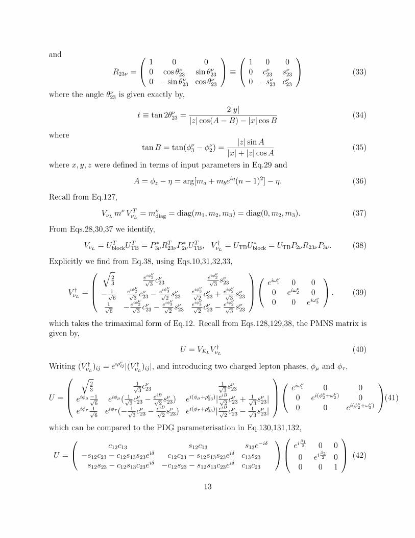
Explicitly we find from Eq.38, using Eqs.10,31,32,33,

V †νL =

√23

eiφν2√3cν23

eiφν2√3sν23

− 1√6

eiφν2√3cν23 − eiφ

ν3√2sν23

eiφν3√2cν23 + eiφ

ν2√3sν23

1√6− eiφ

ν2√3cν23 − eiφ

ν3√2sν23

eiφν3√2cν23 − eiφ

ν2√3sν23

eiων1 0 0

0 eiων2 0

0 0 eiων3

. (39)

which takes the trimaximal form of Eq.12. Recall from Eqs.128,129,38, the PMNS matrix isgiven by,

U = VELV†νL

(40)

Writing (V †νL)ij = eiρνij |(V †νL)ij|, and introducing two charged lepton phases, φµ and φτ ,

U =

√23

1√3cν23

1√3sν23

eiφµ −1√6

eiφµ( 1√3cν23 − eiB√

2sν23) ei(φµ+ρν23)| eiB√

2cν23 + 1√

3sν23|

eiφτ 1√6

eiφτ (− 1√3cν23 − eiB√

2sν23) ei(φτ+ρν33)| eiB√

2cν23 − 1√

3sν23|

eiων1 0 0

0 ei(φν2+ων2 ) 0

0 0 ei(φν2+ων3 )

(41)

which can be compared to the PDG parameterisation in Eq.130,131,132,

U =

c12c13 s12c13 s13e−iδ

−s12c23 − c12s13s23eiδ c12c23 − s12s13s23e

iδ c13s23

s12s23 − c12s13c23eiδ −c12s23 − s12s13c23e

iδ c13c23

eiβ12 0 0

0 eiβ22 0

0 0 1

(42)

13

from which comparison we identify the physical PMNS lepton mixing angles by the exactexpressions

sin θ13 =1√3sν23 =

1√6

(1−

√1

1 + t2

)1/2

(43)

tan θ12 =1√2cν23 =

1√2

(1− 3 sin2 θ13

)1/2(44)

tan θ23 =| eiB√

2cν23 + 1√

3sν23|

| eiB√2cν23 − 1√

3sν23|

=|1 + εν23||1− εν23|

(45)

where we have selected the negative sign for the square root in parentheses, applicable forthe physical range of parameters, and defined

εν23 ≡√

2

3tan θν23e

−iB =

√2

3t−1[√

1 + t2 − 1]e−iB (46)

expressing the results in terms of t ≡ tan 2θν23 and B = φν3 −φν2 which were given in terms ofinput parameters in Eqs.34,35,36. The solar angle tan θ12 approximately takes the TB valueof 1/

√2, to first order in sin θ13. The atmospheric angle tan θ23 is maximal when B = ±π/2

since then |1 + εν23| is equal to |1− εν23|.

9 Exact analytic results for neutrino masses

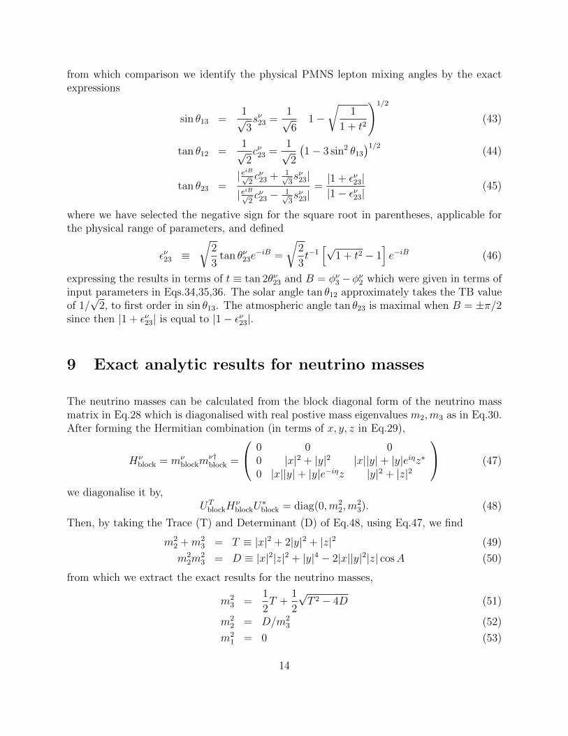
The neutrino masses can be calculated from the block diagonal form of the neutrino massmatrix in Eq.28 which is diagonalised with real postive mass eigenvalues m2,m3 as in Eq.30.After forming the Hermitian combination (in terms of x, y, z in Eq.29),

Hνblock = mν

blockmν†block =

0 0 00 |x|2 + |y|2 |x||y|+ |y|eiηz∗0 |x||y|+ |y|e−iηz |y|2 + |z|2

(47)

we diagonalise it by,UT

blockHνblockU

∗block = diag(0,m2

2,m23). (48)

Then, by taking the Trace (T) and Determinant (D) of Eq.48, using Eq.47, we find

m22 +m2

3 = T ≡ |x|2 + 2|y|2 + |z|2 (49)

m22m

23 = D ≡ |x|2|z|2 + |y|4 − 2|x||y|2|z| cosA (50)

from which we extract the exact results for the neutrino masses,

m23 =

1

2T +

1

2

√T 2 − 4D (51)

m22 = D/m2

3 (52)

m21 = 0 (53)

14

where we have selected the positive sign for the square root which is applicable for m23 > m2

2.Furthermore, since m2

3 � m22 (recall m2

3/m22 ≈ 30 ) we may approximate,

m23 ≈ T = |x|2 + 2|y|2 + |z|2 (54)

m22 ≈ D/T =

|x|2|z|2 + |y|4 − 2|x||y|2|z| cosA

|x|2 + 2|y|2 + |z|2(55)

The sequential dominance (SD) approximation that the atmospheric right-handed neutrinodominates over the solar right-handed neutrino contribution to the seesaw mass matriximplies that ma � mb and |z| � |x|, |y| leading to

m23 ≈ |z|2 −→ m3 ≈ 2ma (56)

m22 ≈ |x|2 −→ m2 ≈ 3mb (57)

using the definitions in Eq.29. The results in Eqs.56 and 57 are certainly very simple, buthow accurate are they? For the CSD(3) numerical benchmark ma ≈ 27 meV and mb ≈ 2.7meV gives m3 ≈ 50 meV, m2 ≈ 8.6 meV. We find |z| ≈ 46 meV , |x| ≈ 8.0 meV (and|y| ≈ 13 meV) which is a reasonable approximation. The SD approximations in Eqs.56and 57 give, m3 ≈ 2ma ≈ 54 meV and m2 ≈ 3mb ≈ 8.1 meV, accurate to say 10%. Theapproximate results in Eqs.54,55 are more accurate to say 3%, with the results in Eqs.51,52being of course exact.

The SD approximation in Eqs.56, 57 is both insightful and useful, since two of the threeinput parameters, namely ma and mb, are immediately fixed by the two physical neutrinomasses m3 and m2, which, for m1 = 0, are identified as the square roots of the measuredmass squared differences ∆m2

31 and ∆m221. This leaves, in the SD approximation, the only

remaining parameters to be n and the phase η, which, together, determine the entire PMNSmixing matrix (3 angles, and 2 phases). For example if n = 3 and η = 2π/3 were determinedby some model, then the PMNS matrix would be determined uniquely, without any freedom,in the SD approximation. When searching for a best fit solution, the SD approximation inin Eqs.56, 57 is useful as a first approximation which enables the parameters ma and mb tobe approximately determined by ∆m2

31 and ∆m221 since this may then be used as a starting

point around which a numerical minimisation package can be run using the exact results forthe neutrino masses in Eqs.51,52 together with the exact results for the lepton mixing anglesin Eqs.43,44,45.

10 Exact analytic results for CP violation

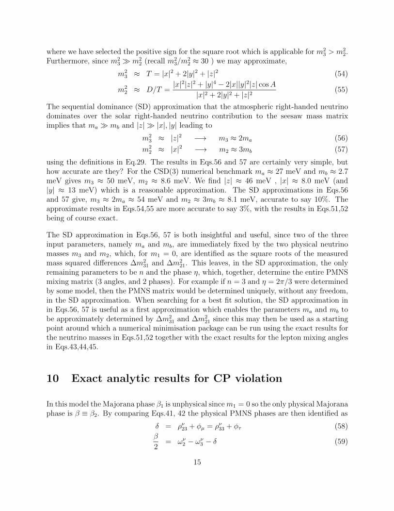
In this model the Majorana phase β1 is unphysical sincem1 = 0 so the only physical Majoranaphase is β ≡ β2. By comparing Eqs.41, 42 the physical PMNS phases are then identified as

δ = ρν23 + φµ = ρν33 + φτ (58)

β

2= ων2 − ων3 − δ (59)

15

Extracting the value of the physical phases δ and β in terms of input parameters is rathercumbersome and it is better to use the Jarlskog and Majorana invariants in order to do this.

10.1 The Jarlskog Invariant

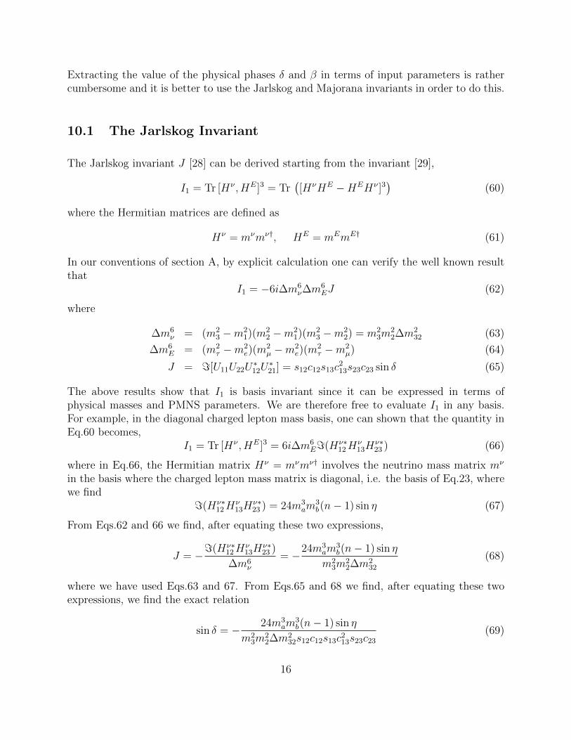
The Jarlskog invariant J [28] can be derived starting from the invariant [29],

I1 = Tr [Hν , HE]3 = Tr([HνHE −HEHν ]3

)(60)

where the Hermitian matrices are defined as

Hν = mνmν†, HE = mEmE† (61)

In our conventions of section A, by explicit calculation one can verify the well known resultthat

I1 = −6i∆m6ν∆m

6EJ (62)

where

∆m6ν = (m2

3 −m21)(m2

2 −m21)(m2

3 −m22) = m2

3m22∆m2

32 (63)

∆m6E = (m2

τ −m2e)(m

2µ −m2

e)(m2τ −m2

µ) (64)

J = =[U11U22U∗12U

∗21] = s12c12s13c

213s23c23 sin δ (65)

The above results show that I1 is basis invariant since it can be expressed in terms ofphysical masses and PMNS parameters. We are therefore free to evaluate I1 in any basis.For example, in the diagonal charged lepton mass basis, one can shown that the quantity inEq.60 becomes,

I1 = Tr [Hν , HE]3 = 6i∆m6E=(Hν∗

12Hν13H

ν∗23 ) (66)

where in Eq.66, the Hermitian matrix Hν = mνmν† involves the neutrino mass matrix mν

in the basis where the charged lepton mass matrix is diagonal, i.e. the basis of Eq.23, wherewe find

=(Hν∗12H

ν13H

ν∗23 ) = 24m3

am3b(n− 1) sin η (67)

From Eqs.62 and 66 we find, after equating these two expressions,

J = −=(Hν∗12H

ν13H

ν∗23 )

∆m6ν

= −24m3am

3b(n− 1) sin η

m23m

22∆m2

32

(68)

where we have used Eqs.63 and 67. From Eqs.65 and 68 we find, after equating these twoexpressions, we find the exact relation

sin δ = − 24m3am

3b(n− 1) sin η

m23m

22∆m2

32s12c12s13c213s23c23

(69)

16

Note the minus sign in Eq.69, which means that, for n > 1, the sign of sin δ takes theopposite value to the sign of sin η, in the convention we use to write our neutrino massmatrix in section A. Since the denominator of Eq.69 may be expressed in terms of inputparameters, using the exact results for the neutrino masses in Eqs.51,52 together with theexact results for the lepton mixing angles in Eqs.43,44,45, it is clear that Eq.69 gives sin δin terms of input parameters in both the numerator and demominator.

In the SD approximation in Eqs.56, 57 we find from Eq.68,

J ≈ −1

9

m2

m3

(n− 1) sin η, (70)

where the minus sign in Eq.70 again clearly shows the anti-sign correlation of sin δ andsin η, where η is the input phase which appears in the neutrino mass matrix in Eq.23 andleptogenesis in Eq.25. In other words the BAU is proportional to − sin δ if the lightestright-handed neutrino is the one dominantly responsible for the atmospheric neutrino massN1 = Natm . In this case the observed matter Universe requires sin δ to be negative in orderto generate a positive BAU. It is interesting to note that, up to a negative factor, the sineof the leptogenesis phase η is equal to the sine of the oscillation phase δ, so the observationthe CP violation in neutrino oscillations is directly responsible for the CP violation in theearly Universe, in the LS model.

10.2 The Majorana Invariant

The Majorana invariant may be defined by [30],

I2 = =Tr [HEmνmν†mνHE∗mν†] (71)

In our conventions of section A, this may be written,

I2 = =Tr [U †HEdiagUm

ν3diagU

THEdiagU

∗mνdiag] (72)

By explicit calculation we find an exact but rather long expression which is basis invariantsince it involves physical masses and PMNS parameters. We do not show the result heresince it is rather long and not very illuminating and also not so relevant since Majorana CPviolation is not going to be measured for a very long time. However, since m2

e � m2µ � m2

τ ,we may neglect m2

e and m2µ compared to m2

τ , and also drop s213 terms, to give the compact

result,I2 ≈ −m4

τm2m3∆m232c

213c

223[c2

12s223(sin β) + 2c12c23s12s13s23 sin(β + δ)]. (73)

Notice that I2 is zero if both β and δ are zero or π, so it is indeed sensitive to MajoranaCP violation arising from β. Indeed I2 is roughly proportional to sin β if the s13 term is alsoneglected,

I2 ≈ −m4τm2m3∆m2

32c213c

223c

212s

223(sin β). (74)

17

We are free to evaluate I2 in any basis. For example, in the diagonal charged lepton massbasis, the quantity in Eq.71 becomes,

I2 = =Tr [HEdiagm

νmν†mνHEdiagm

ν†] (75)

where in Eq.75, the neutrino mass matrix mν is in the basis where the charged lepton massmatrix is diagonal, i.e. the basis of Eq.23. Evaluating Eq.75 we find the exact result,

I2 = mamb sin η[−4m2

a(m2τ −m2

µ)2 +m2b

(m2τ (2n+ 1)(n− 2)−m2

µn(2n− 5)− 2m2e(n− 1)

)2]

(76)If we neglect m2

e and m2µ, Eq.76 becomes approximately,

I2 ≈ m4τmamb sin η

[−4m2

a +m2b(2n+ 1)2(n− 2)2

]. (77)

From Eqs.74 and 77 we find, after equating these two expressions, one finds an approximateformula for the sine of the Majorana phase,

sin β ≈ mamb[4m2a −m2

b(2n+ 1)2(n− 2)2] sin η

m2m3∆m232c

213c

223c

212s

223

(78)

Since the denominator of Eq.78 may be expressed in terms of input parameters, using theexact results for the neutrino masses in Eqs.51,52 together with the exact results for thelepton mixing angles in Eqs.43,44,45, it is clear that Eq.78 gives sin β in terms of inputparameters in both the numerator and demominator. For low values of n (e.g. n = 3) thesign of sin β is the same as the sign of sin η and hence the opposite of the sign of sin δ givenby Eq.69.

It is worth recalling at this point that our Majorana phases are in the convention of Eq.132,

namely P = diag(eiβ12 , ei

β22 , 1), where we defined β = β2 and β1 is unphysical since m1 = 0.

In another common convention the Majorana phases are by given by P = diag(1, eiα212 , ei

α312 ),

which are related to ours by α21 = β2 − β1 and α31 = −β1. For the case at hand, wherem1 = 0, one finds β = α21 − α31 to be the only Majorana phase having any physicalsignificance (e.g. which enters the formula for neutrinoless double beta decay). This is thephase given by Eq.78.

Eq.78 is independent of s13 since we have dropped those terms. It is only therefore expectedto be accurate to about 15%, which is acceptable, given that the Majorana phase β ispractically impossible to measure in the forseeable future for the case of a normal masshierarchy with the lightest neutrino mass m1 = 0. However, if it becomes necessary in thefuture to have a more accurate result, this can be obtained by equating Eq.73 with Eq.77,which would yield an implicit formula for β which is accurate to about 3%:

sin β + 2c−112 c23s12s13s

−123 sin(β + δ) ≈ mamb[4m

2a −m2

b(2n+ 1)2(n− 2)2] sin η

m2m3∆m232c

213c

223c

212s

223

. (79)

18

11 Exact Sum Rules

The formulas in the previous section give the observable physical neutrino masses and thePMNS angles and phases in terms of fewer input parameters ma, mb, n and η. In particular,the exact results for the neutrino masses are given in Eqs.51,52,53, the exact results for thelepton mixing angles are given in Eqs.43,44,45 and the exact result for the CP violating Diracoscillation phase is given in Eq.69, while the Majorana phase is given approximately by Eq.78.These 8 equations for the 8 observables cannot be inverted to give the 4 input parametersin terms of the 8 physical parameters since there are clearly fewer input parameters thanobservables. On the one hand, this is good, since it means that the littlest seesaw has 4predictions, on the other hand it does mean that we have to deal with a 4 dimensionalinput parameter space. Later we shall impose additional theoretical considerations, whichshall reduce this parameter space to just 2 input parameters, yielding 6 predictions, but fornow we consider the 4 input paramaters. In any case it is not obvious that one can deriveany sum rules where input parameters are eliminated, and only relations between physicalobservables remain.

Nevertheless in this model there are such sum rules, i.e. relations between physical observ-ables not involving the input parameters. An example of such a sum rule is Eq.44, which wegive below in three equivalent exact forms,

tan θ12 =1√2

√1− 3s2

13 or sin θ12 =1√3

√1− 3s2

13

c13

or cos θ12 =

√2

3

1

c13

(80)

This sum rule is in fact common to all TM1 models, and is therefore also applicable to theLS models which predict TM1 mixing. Similarly TM1 predicts the so called atmosphericsum rule, also applicable to the LS models. This arises from the fact that the first columnof the PMNS matrix is the same as the first column of the TB matrix in Eq.10. Indeed, bycomparing the magnitudes of the elements in the first column of Eq.41 to those in the firstcolumn of Eq.42, we obtain,

|Ue1| = c12c13 =

√2

3(81)

|Uµ1| = | − s12c23 − c12s13s23eiδ| =

√1

6(82)

|Uτ1| = |s12s23 − c12s13c23eiδ| =

√1

6(83)

Eq.81 is equivalent to Eq.80 while Eqs.82 and 83 lead to equivalent mixing sum rules whichcan be expressed as an exact relation for cos δ in terms of the other lepton mixing angles[21],

cos δ = − cot 2θ23(1− 5s213)

2√

2s13

√1− 3s2

13

(84)

19

Note that, for maximal atmospheric mixing, θ23 = π/4, we see that cot 2θ23 = 0 and thereforethis sum rule predicts cos δ = 0, corresponding to maximal CP violation δ = ±π/2. Theprospects for testing the TM1 atmospheric sum rules Eqs.80,84 in future neutrino facilitieswas discussed in [31].

The LS model also the predicts additional sum rules beyond the TM1 sum rules that arisefrom the structure of the Dirac mass matrix in Eq.20. Recalling that the PMNS matrixis written in Eq.130 as U = V P , where V is the the CKM-like part and P contains theMajorana phase β, the LS sum rules are [10],

|Vµ3Ve2 − Vµ2Ve3||Vτ3Ve2 − Vτ2Ve3|

= 1 (85)

|eiβm2Vµ2Ve2 +m3Vµ3Ve3||eiβm2V 2

e2 +m3V 2e3|

= n (86)

|eiβm2Vτ2Ve2 +m3Vτ3Ve3||eiβm2V 2

e2 +m3V 2e3|

= n− 2 (87)

where the sum rule in Eq.85 is independent of both n and β. We emphasise again that thematrix elements Vαi refer to the first matrix on the right-hand side of Eq.42 (i.e. withoutthe Majorana matrix). Of course similar relations apply with U replacing V everywhere andthe Majorana phase β disappearing, being absorbed into the PMNS matrix U , but we preferto exhibit the Majorana phase dependence explicitly. However the LS sum rule in Eq.85 isequivalent to the TM1 sum rule in Eq.84, as seen by explicit calculation. The other LS sumrules in Eqs.86 and 87 involve the phase β and are not so interesting.

12 The reactor and atmospheric angles

Since the solar angle is expected to be very close to its tribimaximal value, according to theTM1 sum rules in Eq.80, independent of the input parameters, in this section we focus onthe analytic predictions for the reactor and atmospheric angles, starting with the accuratelymeasured reactor angle which is very important for pinning down the input parameters ofthe LS model.

12.1 The reactor angle

The exact expression for the reactor angle in Eq.43 is summarised below,

sin θ13 =1√6

(1−

√1

1 + t2

)1/2

, (88)

20

where from Eqs. 29,34,35,36,

t =2√

6mb(n− 1)

2|ma +mbeiη(n− 1)2| cos(A−B)− 3mb cosB(89)

where

tanB =2|ma +mbe

iη(n− 1)2| sinA3mb + 2|ma +mbeiη(n− 1)2| cosA

(90)

andA = arg[ma +mbe

iη(n− 1)2]− η. (91)

The above results are exact and necessary for precise analysis of the model, especially forlarge n (where n is in general a real and continuous number). We now proceed to derivesome approxinate formulae which can give useful insight.

The SD approximations in Eqs.56,57 show that mb/ma ≈ (2/3)m2/m3. This suggests thatwe can make an expansion in mb/ma, or simply drop mb compared to ma, as a leadingorder approximation, which implies tanB ≈ tanA and hence cos(A − B) ≈ 1. Thus Eq.89becomes,

t ≈√

6mb(n− 1)

|ma +mbeiη(n− 1)2|(92)

where we have kept the term proportional to mb(n− 1)2, since the smallness of mb may becompensated by the factor (n−1)2 for n > 1. Eq.92 shows that t� 1, hence we may expandEq.88 to leading order in t,

sin θ13 ≈t

2√

3+O(t3). (93)

Hence combining Eqs.92 and 93, we arrive at our approximate form for the sine of the reactorangle,

sin θ13 ≈1√2

mb(n− 1)

|ma +mbeiη(n− 1)2|. (94)

For low values of (n− 1) such that mb(n− 1)2 � ma, Eq.94 simplifies to,

sin θ13 ≈ (n− 1)

√2

3

m2

m3

(95)

using the SD approximations in Eqs.56,57 that mb/ma ≈ (2/3)m2/m3, valid to 10% accuracy.For example, the result shows that for the original CSD [8], where n = 1, implies sin θ13 = 0,

while for CSD(2) [9] (i.e. n = 2) we have sin θ13 ≈√

23m2

m3, leading to θ13 ≈ 4.7◦ which is too

small. For CSD(3) [10] (i.e. n = 3) we have sin θ13 ≈ 2√

23

m2

m3, leading to θ13 ≈ 9.5◦, in rough

agreement with the observed value of θ13 ≈ 8.5◦, within the accuracy of our approximations.We conclude that these results show how sin θ13 ∼ O(m2/m3) can be achieved, with valuesincreasing with n, and confirm that n ≈ 3 gives the best fit to the reactor angle. Weemphasise that the approximate formula in Eq.95 has not been written down before, andthat the exact results in Eqs.88,89,90,91 are also new and in perfect agreement with thenumerical results in Table 1.

21

12.2 The atmospheric angle

The exact expression for the atmospheric angle in Eq.45 is summarised below,

tan θ23 =|1 + εν23||1− εν23|

(96)

where

εν23 =

√2

3t−1[√

1 + t2 − 1]e−iB (97)

and t and B were summarised in Eqs.89,90,91. The above results, which are exact, showthat the atmospheric angle is maximal for B ≈ ±π/2, as noted previously.

We may expand Eq.97 to leading order in t,

εν23 ≈t√6e−iB +O(t3). (98)

Hence combining Eqs.96,98, we arrive at an approximate form for the tangent of the atmo-spheric angle,

tan θ23 ≈|1 + t√

6e−iB|

|1− t√6e−iB|

≈ 1 + 2t√6

cosB, (99)

where t was approximated in Eq.92. We observed earlier that, for mb � ma, tanB ≈ tanAand hence A ≈ B. Unfortunately it is not easy to obtain a reliable approximation for A inEq.91, unless n >∼ 1 in which case A ≈ −η. However, for n−1 significantly larger than unity,this is not a good approximation. For example for n = 3 from Eq.91 we have,

A = arg[ma + 4mbeiη]− η (100)

Taking mb/ma = 1/10, this gives

A = arg[1 + 0.4eiη]− η (101)

which shows that A ≈ −η is not a good approximation even though mb � ma. If we set, forexample, η = 2π/3, as in Table 1, then Eq.101 gives

A = 0.41− 2π/3 ≈ −0.53π (102)

which happens to be close to −π/2. Hence, since A ≈ B, this choice of parameters impliescosB ≈ 0, leading to approximately maximal atmospheric mixing from Eq.99, as observedin Table 1. At this point it is also worth recalling that for maximal atmospheric mixing, theTM1 sum rule in Eq.84 predicts that the cosine of the CP phase δ to be zero, correspondingto maximal Dirac CP violation δ = ±π/2, as approximately found in Table 1.

22

13 CSD(3) vacuum alignments from S4

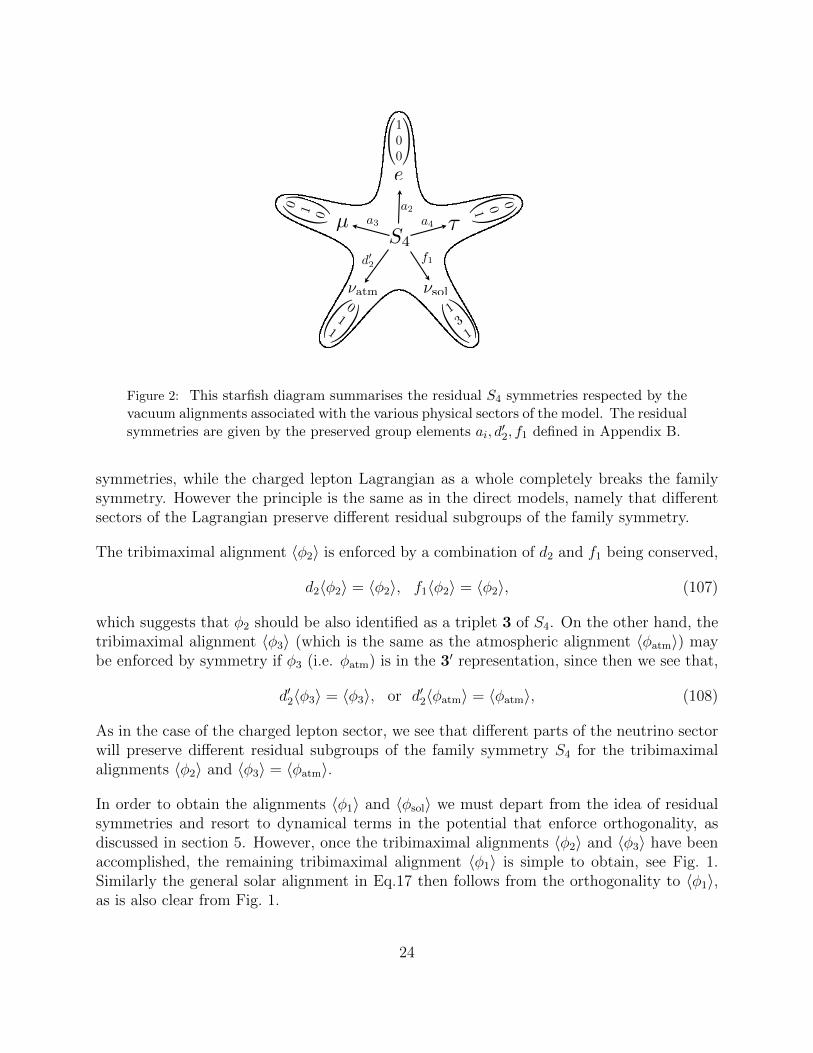
We saw from the discussion of the reactor angle, and in Table 1, that the solar alignmentin Eq.17 for the particular choice n = 3 was favoured. In this section we show how thedesired alignments for n = 3 can emerge from S4 due to residual symmetries. Although thecharged lepton alignments we discuss were also obtained previously from A4 [10], the neutrinoalignments in Eq.17 for n = 3 were not previously obtained from residual symmetries, andindeed we will see that they will arise from group elements which appear in S4 but not A4.

We first summarise the vacuum alignments that we desire:

〈φatm〉 = vatm

011

, 〈φsol〉 = vsol

131

, (103)

in the neutrino sector as in Eq.17 with n = 3, and,

〈ϕe〉 = ve

100

, 〈ϕµ〉 = vµ

010

, 〈ϕτ 〉 = vτ

001

. (104)

in the charged lepton sector.

For comparison we also give the tribimaximal alignments in Eq.14:

〈φ1〉 = v1

2−11

, 〈φ2〉 = v2

11−1

, 〈φ3〉 = v3

011

. (105)

We first observe that the charged lepton and the tribimaximal alignments individually pre-serve some remnant symmetry of S4, whose triplet representations are displayed explicitlyin Appendix B. If we regard ϕe, ϕµ, ϕτ as each being a triplet 3 of S4, then they eachcorrespond to a different symmetry conserving direction of S4, with,

a2〈ϕe〉 = 〈ϕe〉, a3〈ϕµ〉 = 〈ϕµ〉, a4〈ϕτ 〉 = 〈ϕτ 〉. (106)

One may question the use of different residual symmetry generators of S4 to enforce thedifferent charged lepton vacuum alignments. However, this is analagous to what is usuallyassumed in the direct model building approach when one says that the charged lepton sec-tor preserves one residual symmetry, while the neutrino sector preserves another residualsymmetry. In the direct case, it is clear that the lepton Lagrangian as a whole completelybreaks the family symmetry, even though the charged lepton and neutrino sectors preservedifferent residual symmetries. In the indirect case here, we are taking this argument onestep further, by saying that the electron, muon and tau sectors preserve different residual

23

S4

0@

100

1A

0 @0 1 0

1 A0@

001 1A

0@ 01

1

1A

0@1

31

1A

e

µ ⌧

⌫atm ⌫sol

a2

a3 a4

d02 f1

Figure 2: This starfish diagram summarises the residual S4 symmetries respected by thevacuum alignments associated with the various physical sectors of the model. The residualsymmetries are given by the preserved group elements ai, d

′2, f1 defined in Appendix B.

symmetries, while the charged lepton Lagrangian as a whole completely breaks the familysymmetry. However the principle is the same as in the direct models, namely that differentsectors of the Lagrangian preserve different residual subgroups of the family symmetry.

The tribimaximal alignment 〈φ2〉 is enforced by a combination of d2 and f1 being conserved,

d2〈φ2〉 = 〈φ2〉, f1〈φ2〉 = 〈φ2〉, (107)

which suggests that φ2 should be also identified as a triplet 3 of S4. On the other hand, thetribimaximal alignment 〈φ3〉 (which is the same as the atmospheric alignment 〈φatm〉) maybe enforced by symmetry if φ3 (i.e. φatm) is in the 3′ representation, since then we see that,

d′2〈φ3〉 = 〈φ3〉, or d′2〈φatm〉 = 〈φatm〉, (108)

As in the case of the charged lepton sector, we see that different parts of the neutrino sectorwill preserve different residual subgroups of the family symmetry S4 for the tribimaximalalignments 〈φ2〉 and 〈φ3〉 = 〈φatm〉.

In order to obtain the alignments 〈φ1〉 and 〈φsol〉 we must depart from the idea of residualsymmetries and resort to dynamical terms in the potential that enforce orthogonality, asdiscussed in section 5. However, once the tribimaximal alignments 〈φ2〉 and 〈φ3〉 have beenaccomplished, the remaining tribimaximal alignment 〈φ1〉 is simple to obtain, see Fig. 1.Similarly the general solar alignment in Eq.17 then follows from the orthogonality to 〈φ1〉,as is also clear from Fig. 1.

24

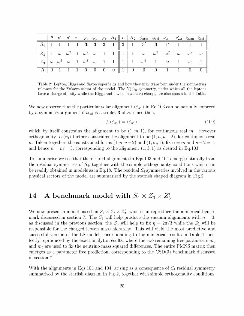
θ ec µc τ c ϕe ϕµ ϕτ H1 L H2 φatm φsol νcatm νcsol ξatm ξsol

S4 1 1 1 1 3 3 3 1 3 1 3′ 3 1′ 1 1 1

Z3 1 ω ω2 1 ω2 ω 1 1 1 1 ω ω2 ω2 ω ω2 ω

Z ′3 ω ω2 ω 1 ω2 ω 1 1 1 1 ω2 1 ω 1 ω 1

R 0 1 1 1 0 0 0 0 1 0 0 0 1 1 0 0

Table 2: Lepton, Higgs and flavon superfields and how they may transform under the symmetriesrelevant for the Yukawa sector of the model. The U(1)R symmetry, under which all the leptonshave a charge of unity while the Higgs and flavons have zero charge, are also shown in the Table.

We now observe that the particular solar alignment 〈φsol〉 in Eq.103 can be natually enforcedby a symmetry argument if φsol is a triplet 3 of S4 since then,

f1〈φsol〉 = 〈φsol〉, (109)

which by itself constrains the alignment to be (1,m, 1), for continuous real m. Howeverorthogonality to 〈φ1〉 further constrains the alignment to be (1, n, n− 2), for continuous realn. Taken together, the constrained forms (1, n, n−2) and (1,m, 1), fix n = m and n−2 = 1,and hence n = m = 3, corresponding to the alignment (1, 3, 1) as desired in Eq.103.

To summarise we see that the desired alignments in Eqs.103 and 104 emerge naturally fromthe residual symmetries of S4, together with the simple orthogonality conditions which canbe readily obtained in models as in Eq.18. The residual S4 symmetries involved in the variousphysical sectors of the model are summarised by the starfish shaped diagram in Fig.2.

14 A benchmark model with S4 × Z3 × Z ′3

We now present a model based on S4 × Z3 × Z ′3, which can reproduce the numerical bench-mark discussed in section 7. The S4 will help produce the vacuum alignments with n = 3,as discussed in the previous section, the Z3 will help to fix η = 2π/3 while the Z ′3 will beresponsible for the charged lepton mass hierarchy. This will yield the most predictive andsuccessful version of the LS model, corresponding to the numerical results in Table 1, per-fectly reproduced by the exact analytic results, where the two remaining free parameters ma

and mb are used to fix the neutrino mass squared differences. The entire PMNS matrix thenemerges as a parameter free prediction, corresponding to the CSD(3) benchmark discussedin section 7.

With the alignments in Eqs.103 and 104, arising as a consequence of S4 residual symmetry,summarised by the starfish diagram in Fig.2, together with simple orthogonality conditions,

25

as further discussed in the next section, we may write down the superpotential of the starfishlepton model, as a supersymmetric version 3 of the LS Lagrangian in Eq.19,

W yukS4

=1

ΛH2(L.φatm)νcatm +

1

ΛH2(L.φsol)ν

csol + ξatmν

catmν

catm + ξsolν

csolν

csol (110)

+1

ΛH1(L.ϕτ )τ

c +1

Λ2θH1(L.ϕµ)µc +

1

Λ3θ2H1(L.ϕe)e

c (111)

where only these terms are allowed by the charges in Table 2, where L are the three familiesof electroweak lepton doublets unified into a single triplet of S4, νcatm and νcsol are the (CPconjugated) right-handed neutrinos which are singlets of S4, as are the two Higgs doubletsH1,2, while φi and ϕα are S4 triplet scalar flavons with the vacuum alignments in Eqs.103and 104. Note that, according to the arguments of the previous section, all flavons are in the3 representation apart from the atmospheric flavon which must be in the 3′ which impliesthat the atmospheric right-handed neutrino must be in the 1′ of S4. We have introducedMajoron singlets ξi whose VEVs will generate the diagonal right-handed neutrino masses.We have suppressed all dimensionless Yukawa coupling constants, assumed to be of orderunity, with the charged lepton mass hierarchy originating from powers of θ which is an S4

singlet. The corresponding powers of the mass scale Λ keeps track of the mass dimension ofeach term.

Inserting the vacuum alignments in Eqs.103 and 104 into Eqs.110 and 111, we obtain theneutrino and charged lepton Yukawa matrices, with the rigid CSD(3) structure,

Y ν =

0 ysol

yatm 3ysol

yatm ysol

, Y E =

ye 0 00 yµ 00 0 yτ

, (112)

where

yatm ∼vatm

Λ, ysol ∼

vsol

Λ, yτ ∼

vτΛ, yµ ∼

vµ〈θ〉Λ2

, ye ∼ve〈θ〉2

Λ3. (113)

Note that we have a qualitative understanding of the charged lepton mass hierarchy as beingdue to successive powers of θ, but there is no predictive power (for charged lepton masses) dueto the arbitrary flavon VEVs and undetermined order unity dimensionless Yukawa couplingswhich we suppress.

When the Majorons get VEVs, the last two terms in Eq.110 will lead to the diagonal heavyMajorana mass matrix,

MR =

(Matm 0

0 Msol

), (114)

3It is trivial to convert this superpotential to a non-supersymmetric Lagrangian by interpreting the leptonsas fermions and the Higgs and flavons as scalars, rather than superfields. In the non-supersymmetric case itis possible to identify H2 as the CP conjugate of the Higgs doublet H1. It is also possible to absorb this Higgsdoublet into the flavon fields so that φi and ϕα represent five S4 triplets of Higgs doublets, correspondingto 15 Higgs doublets, in which case one power of Λ would be removed from the denominator each term.

26

where Matm ∼ 〈ξatm〉 and Msol ∼ 〈ξsol〉. With the above seesaw matrices, we now have allthe ingredients to reproduce the CSD(3) benchmark neutrino mass matrix in Eq. 24, apartfrom the origin of the phase η = 2π/3, which arises from vacuum alignment as we discuss inthe next section.

15 Vacuum alignment in the S4 × Z3 × Z ′3 model

We have argued in section 13 that in general the vacuum the alignments in Eqs.103 and104, arise as a consequence of S4 residual symmetry, summarised by the starfish diagram inFig.2, together with simple orthogonality conditions. It remains to show how this can beaccomplished, together with the Majoron VEVs, by explicit superpotential alignment terms.

The charged lepton alignments in Eq.104 which naturally arise as a consequence of S4, canbe generated from the simple terms,

W flav,`S4

= Aeϕeϕe + Aµϕµϕµ + Aτϕτϕτ . (115)

where Al are S4 triplet 3 driving fields with necessary Z3×Z ′3 charges to absorb the chargesof φl so as to allow the terms in Eq.115. F-flatness then leads to the desired charged leptonflavon alignments in Eq.104 due to,

〈φl〉2〈φl〉3〈φl〉3〈φl〉1〈φl〉1〈φl〉2

=

000

(116)

for l = e, µ, τ .

The vacuum alignment of the neutrino flavons involves the additional tribimaximal flavonsφi with the orthogonality terms in Eq.18,

W flav,perpS4

= Oijφiφj +Osolφsolφ1 (117)

where we desire the tribimaximal alignments in Eq.105 and as usual we identify φatm ≡ φ3.We shall assume CP conservation with all triplet flavons acquiring real CP conserving VEVs.Since there is some freedom in the choice of φ1,2 charges under Z3 × Z ′3, we leave themunspecified. The singlet driving fields Oij and Osol have R = 2 and Z3×Z ′3 charges fixed bythe (unspecified) φi charges,

The tribimaximal alignment for φ2 in the 3 in Eq.105 naturally arises as a consequence ofS4 from the simple terms,

W flav,TB2S4

= A2(g2φ2φ2 + g′2φ2ξ2). (118)

27

where A2 is an R = 2, S4 triplet 3 driving field and ξ2 is a singlet, with the same (unspecified)Z3 × Z ′3 charge as φ2. F-flatness leads to,

2g2

〈φ2〉2〈φ2〉3〈φ2〉3〈φ2〉1〈φ2〉1〈φ2〉2

+ g′2〈ξ2〉

〈φ2〉1〈φ2〉2〈φ2〉3

=

000

, (119)

leading to the tribimaximal alignment for φ2 in Eq.105. Note that in general the alignmentderived from these F -term conditions is 〈φ2〉 ∝ (±1,±1,±1)T . These are all equivalent. Forexample (1, 1,−1) is related to permutations of the minus sign by S4 transformations. Theother choices can be obtained from these by simply multiplying an overall phase which wouldalso change the sign of the ξ2 VEV.

The tribimaximal alignment for φatm ≡ φ3 in the 3′ in Eq.105 naturally arises from

W flav,atmS4

= A3(g3φ3φ3 + g′3φeξ3), (120)

where A3 is an S4 triplet 3 driving field and ξ3 is a singlet, with suitable Z3 × Zθ3 charges

assigned to all the fields so as to allow only these terms. F-flatness leads to,

2g3

〈φ3〉2〈φ3〉3〈φ3〉3〈φ3〉1〈φ3〉1〈φ3〉2

+ g′3〈ξ2〉

〈φe〉1〈φe〉2〈φe〉3

=

000

, (121)

which, using the orthogonality of φ2 and φ3 using Eq.117 and the pre-aligned electron flavonin Eq.104, leads to the tribimaximal alignment for φatm ≡ φ3 in Eq.105. The tribimaxi-mal alignment for φ1 then follows directly from the orthogonality conditions resulting fromEq.117.

The solar flavon alignment comes from the terms,

W flav,solS4

= Asol(gsolφsolφsol + g′solφsolξ′sol + gµφµξµ). (122)

F-flatness leads to,

2gsol

〈φsol〉2〈φsol〉3〈φsol〉3〈φsol〉1〈φsol〉1〈φsol〉2

+ g′sol〈ξ′sol〉

〈φsol〉1〈φsol〉2〈φsol〉3

+ gµ〈ξµ〉

〈φµ〉1〈φµ〉2〈φµ〉3

=

000

, (123)

which, using the pre-aligned muon flavon in Eq.104, leads to the form (1,m, 1) for 〈φsol〉,with m unspecified, depending on the muon flavon VEV. On the other hand the last term inEq.117 gives the general CSD(n) form in Eq.17, (1, n, n− 2) for 〈φsol〉. The two constrainedforms (1, n, n− 2) and (1,m, 1), taken together, imply the unique alignment (1, 3, 1) for φsol

in Eq.103.

28

To understand the origin of the phase η = 2π/3 we shall start by imposing exact CPinvariance on the high energy theory, in Eqs.110 and 111, then spontaneously break CP in avery particular way, governed by the Z3 symmetry, so that η is restricted to be a cube rootof unity. The Majoron flavon VEVs are driven by the superpotential,

W flav,majS4

= P

(ξ3

atm

Λ−M2

)+ P ′

(ξ3

sol

Λ′−M ′2

), (124)

where P, P ′ are two copies of “driving” superfields with R = 2 but transforming as singletsunder all other symmetries, and M is real due to CP conservation. Due to F-flatness,

∣∣∣∣〈ξatm〉3

Λ−M2

∣∣∣∣2

=

∣∣∣∣〈ξsol〉3

Λ′−M ′2

∣∣∣∣2

= 0. (125)

These are satisfied by 〈ξatm〉 = |(ΛM2)1/3| and 〈ξsol〉 = |(Λ′M ′2)1/3|e−2iπ/3 where we arbitrar-ily select the phases to be zero and −2π/3 from amongst a discrete set of possible choicesin each case. More generally we require a phase difference of 2π/3 since the overall phaseis not physically relevant, which would happen one in three times by chance. In the basiswhere the right-handed neutrino masses are real and positive this is equivalent to η = 2π/3in Eq.23, as in the benchmark model in Eq.24, due to the see-saw mechanism.

16 Conclusion

The seesaw mechanism provides an elegant explanation of the smallness of neutrino masses.However in general it is difficult to test the mechanism experimentally, since the right-handed Majorana masses may have very large masses out of reach of high energy colliders.The heavy Majorana sector also introduces a new flavour sector, with yet more parameters,beyond those describing low energy neutrino physics. This is of serious concern, since theseesaw mechanism may be our best bet for extending the Standard Model to include neutrinomasses.

Given that the seesaw mechanism is an elegant but practically untestable mechanism witha large number of parameters, in this paper we have relied on theoretical desiderata suchas naturalness, minimality and predictability to guide us towards what we call the “LittlestSeesaw” model which is essentially the two right-handed neutrino model bundled togetherwith further assumptions about the structure of the Yukawa couplings that we call CSD(n).Understandably one should be wary of such assumptions, indeed such principles of natu-ralness and minimality without experimental guidance could well prove to be unreliable.However we are encouraged by the fact that such principles in the guise of sequential domi-nance with a single texture zero, led to the bound θ13 . m2/m3, suggesting a large reactorangle a decade before it was measured. The additional CSD(n) assumptions discussed hereare simply designed to explain why this bound is saturated.

29

It is worth recapping the basic idea of sequential dominance that one of the right-handedneutrinos is dominantly responsible for the atmospheric neutrino mass, while a subdominantright-handed neutrino accounts for the solar neutrino mass, with possibly a third right-handed neutrino being approximately decoupled, leading to an effective two right-handedneutrino model. This simple idea leads to equally simple predictions which makes the schemefalsifiable. Indeed, the litmus test of such sequential dominance is Majorana neutrinos witha normal neutrino mass hiearchy and a very light (or massless) neutrino. These predictionswill be tested soon.

In order to understand why the reactor angle bound is approximately saturated, we needto make additional assumptions, as mentioned. Ironically, the starting point is the originalidea of constrained sequential dominance (CSD) which proved to be a good explanation ofthe tri-bimaximal solar and atmospheric angles but predicted a zero reactor angle. However,this idea can be generalised to the “Littlest Seesaw” comprising a two right-handed neutrinomodel with constrained Yukawa couplings of a particular CSD(n) structure, where heren > 1 is taken to be a real parameter. We have shown that the reactor angle is given byθ13 ∼ (n − 1)

√2

3m2

m3so that n = 1 coresponds to original CSD with θ13 = 0, while n = 3

corresponds to CSD(3) with θ13 ∼ 2√

23m2

m3, corresponding to θ13 ∼ m2/m3, which provides

an explanation for why the SD bound is saturated as observed for this case, with both theapproximation and SD breaking down for large n.

In general, the Littlest Seesaw is able to give a successful desciption of neutrino mass and thePMNS matrix in terms of four input parameters appearing in Eq.23 where the reactor anglerequires n ≈ 3. It predicts a normally ordered and very hierarchical neutrino mass spectrumwith the lightest neutrino mass being zero. It also predicts TM1 mixing with the atmosphericsum rules providing further tests of the scheme. Interestingly the single input phase η must beresponsible for CP violation in both neutrino oscillations and leptogenesis, providing the mostdirect link possible between these two phenomena. Indeed η is identified as the leptogenesisphase. Another input parameter is mb which is identied with the neutrinoless double betadecay observable mee, although this is practically impossible to measure for m1 = 0.

The main conceptual achievement in this paper is to realise that making n continuous greatlysimplifies the task of motivating the CSD(n) pattern of couplings, which emerge almost assimply as the TB couplings, as explained in Fig.1. The main technical achievement of thepaper is to provide exact analytic formulae for the lepton mixing angles, neutrino massesand CP phases in terms of the four input parameters of CSD(n) for any real n > 1. Theexact analytic results should facilitate phenomenological studies of the LS model. We havechecked our analytic results against the numerical bechmark and validated them withinthe numerical precision. We also provided new simple analytic approximations such as:θ13 ∼ (n−1)

√2

3m2

m3where m3 ≈ 2ma and m2 ≈ 3mb. The main model building achievement is

to realise that the successful benchmark LS model based on CSD(3) is quite well motivatedby a discrete S4 symmetry, since the neutrino vacuum alignment directions are enforced byresidual symmetries that are contained in S4, but not A4, which has hitherto been widely

30

used in CSD(n) models. This is illustrated by the starfish diagram in Fig,2. In order to alsofix the input leptogenesis phase to its benchmark value η = 2π/3, we proposed a benchmarkmodel, including supersymmetric vacuum alignment, based on S4×Z3×Z ′3, which representsthe simplest predictive seesaw model in the literature. The resulting benchmark predictionsare: solar angle θ12 = 34◦, reactor angle θ13 = 8.7◦, atmospheric angle θ23 = 46◦, and Diracphase δCP = −87◦. These predictions are all within the scope of future neutrino facilities,and may provide a useful target for them to aim at.

SFK acknowledges partial support from the STFC Consolidated ST/J000396/1 grant andthe European Union FP7 ITN-INVISIBLES (Marie Curie Actions, PITN- GA-2011-289442).

A Lepton Mixing Conventions

In the convention where the effective Lagrangian is given by 4

L = −ELmEER −1

2νLm

ννcL +H.c. . (126)

Performing the transformation from the flavour basis to the real positive mass basis by,

VELmE V †ER = mE

diag = diag(me,mµ,mτ ), VνLmν V T

νL= mν

diag = diag(m1,m2,m3), (127)

the PMNS matrix is given by

U = VELV†νL. (128)

Since we are in the basis where the charged lepton mass matrix mE is already diagonal, thenin general VEL can only be a diagonal matrix,

VEL = PE =

eiφe 0 00 eiφµ 00 0 eiφτ

, (129)

consisting of arbitrary phases, where an identical phase rotation on the right-handed chargedleptons VER = PE leaves the diagonal charged lepton masses in mE unchanged. In practicethe phases in PE are chosen to absorb three phases from the unitary matrix V †νL and to putU in a standard convention [32],

U = V P (130)

4Note that this convention for the light effective Majorana neutrino mass matrix mν differs by an overallcomplex conjugation compared to some other conventions in the literature.

31

where, analogous to the CKM matrix,

V =

c12c13 s12c13 s13e−iδ

−s12c23 − c12s13s23eiδ c12c23 − s12s13s23e

iδ c13s23

s12s23 − c12s13c23eiδ −c12s23 − s12s13c23e

iδ c13c23

, (131)

and the Majorana phase matrix factor is,

P =

eiβ12 0 0

0 eiβ22 0

0 0 1

. (132)

From Eqs.127,128,129, we find,

U †PEmνPEU

∗ = diag(m1,m2,m3). (133)

B S4

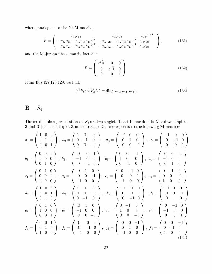
The irreducible representations of S4 are two singlets 1 and 1′, one doublet 2 and two triplets3 and 3′ [33]. The triplet 3 in the basis of [33] corresponds to the following 24 matrices,

a1 =

1 0 00 1 00 0 1

, a2 =

1 0 00 −1 00 0 −1

, a3 =

−1 0 00 1 00 0 −1

, a4 =

−1 0 00 −1 00 0 1

b1 =

0 0 11 0 00 1 0

, b2 =

0 0 1−1 0 00 −1 0

, b3 =

0 0 −11 0 00 −1 0

, b4 =

0 0 −1−1 0 00 1 0

c1 =

0 1 00 0 11 0 0

, c2 =

0 1 00 0 −1−1 0 0

, c3 =

0 −1 00 0 1−1 0 0

, c4 =

0 −1 00 0 −11 0 0

d1 =

1 0 00 0 10 1 0

, d2 =

1 0 00 0 −10 −1 0

, d3 =

−1 0 00 0 10 −1 0

, d4 =

−1 0 00 0 −10 1 0

e1 =

0 1 01 0 00 0 1

, e2 =

0 1 0−1 0 00 0 −1

, e3 =

0 −1 01 0 00 0 −1

, e4 =

0 −1 0−1 0 00 0 1

f1 =

0 0 10 1 01 0 0

, f2 =

0 0 10 −1 0−1 0 0

, f3 =

0 0 −10 1 0−1 0 0

, f4 =

0 0 −10 −1 01 0 0

(134)

32

where ai, bi, ci are the 12 matrices of the A4 triplet representation, while the remaining 12matrices di, ei, fi are the extra matrices in S4. The triplet 3′ in the basis of [33] correspondsto matrices which are are simply related to those above,

a′1 = a1, a′2 = a2, a′3 = a3, a′4 = a4,

b′1 = b1, b′2 = b2, b′3 = b3, b′4 = b4,

c′1 = c1, c′2 = c2, c′3 = c3, c′4 = c4,

d′1 = −d1, d′2 = −d2, d′3 = −d3, d′4 = −d4,

e′1 = −e1, e′2 = −e2, e′3 = −e3, e′4 = −e4,

f ′1 = −f1, f ′2 = −f2, f ′3 = −f3, f ′4 = −f4. (135)

In other words, for the 3′, the 12 matrices a′i, b′i, c′i associated with those of A4 do not change

sign, while the remaining 12 matrices d′i, e′i, f′i involve a change of sign relative to the .

The Kronecker products of S4 are: 1×1 = 1, 1′×1′ = 1, 1′×1 = 1′, 3×3 = 1+2+3+3′,3′ × 3′ = 1 + 2 + 3 + 3′, 3× 3′ = 1′ + 2 + 3 + 3′, 2× 2 = 1 + 1′ + 2, 2× 3 = 3 + 3′,2× 3′ = 3 + 3′. The Clebsch relations in this basis are given in [33].

References

[1] S. F. King, J. Phys. G: Nucl. Part. Phys. 42 (2015) 123001 [arXiv:1510.02091];S. F. King, A. Merle, S. Morisi, Y. Shimizu and M. Tanimoto, New J. Phys. 16 (2014)045018 [arXiv:1402.4271]; S. F. King and C. Luhn, Rept. Prog. Phys. 76 (2013) 056201[arXiv:1301.1340]; S. F. King, Rept. Prog. Phys. 67 (2004) 107 [hep-ph/0310204].

[2] P. Minkowski, Phys. Lett. B 67 (1977) 421; M. Gell-Mann, P. Ramond and R. Slanskyin Sanibel Talk, CALT-68-709, Feb 1979, and in Supergravity, North Holland, Ams-terdam (1979); T. Yanagida in Proc. of the Workshop on Unified Theory and BaryonNumber of the Universe, KEK, Japan (1979); S.L.Glashow, Cargese Lectures (1979);R. N. Mohapatra and G. Senjanovic, Phys. Rev. Lett. 44 (1980) 912; J. Schechter andJ. W. F. Valle, Phys. Rev. D 22 (1980) 2227.

[3] S. F. King, arXiv:1511.03831 [hep-ph].

[4] S. F. King, Phys. Lett. B 439 (1998) 350 [hep-ph/9806440]; S. F. King, Nucl. Phys. B562 (1999) 57 [hep-ph/9904210];

[5] S. F. King, Nucl. Phys. B 576 (2000) 85 [hep-ph/9912492].

[6] S. F. King, JHEP 0209 (2002) 011 [hep-ph/0204360]; S. F. King, Phys. Rev. D 67(2003) 113010 [hep-ph/0211228].

33

[7] P. F. Harrison, D. H. Perkins and W. G. Scott, Phys. Lett. B 530 (2002) 167 [hep-ph/0202074].

[8] S. F. King, JHEP 0508 (2005) 105 [hep-ph/0506297].

[9] S. Antusch, S. F. King, C. Luhn and M. Spinrath, Nucl. Phys. B 856 (2012) 328[arXiv:1108.4278].

[10] S. F. King, JHEP 1307 (2013) 137 [arXiv:1304.6264].

[11] S. F. King, Phys. Lett. B 724 (2013) 92 [arXiv:1305.4846].

[12] S. F. King, JHEP 1401 (2014) 119 [arXiv:1311.3295 [hep-ph]];

[13] S. F. King, JHEP 1408 (2014) 130 [arXiv:1406.7005 [hep-ph]].

[14] F. Bjorkeroth and S. F. King, to be published in J.Phys.G, arXiv:1412.6996 [hep-ph].

[15] F. Bjorkeroth, F. J. de Anda, I. de Medeiros Varzielas and S. F. King, JHEP 1506(2015) 141 [arXiv:1503.03306 [hep-ph]].

[16] F. Bjorkeroth, F. J. de Anda, I. Medeiros de Varzielas and S. F. King, JHEP 1510(2015) 104 [arXiv:1505.05504 [hep-ph]].

[17] F. Bjrkeroth, F. J. de Anda, I. d. M. Varzielas and S. F. King, arXiv:1512.00850 [hep-ph].

[18] P. H. Frampton, S. L. Glashow and T. Yanagida, Phys. Lett. B 548 (2002) 119 [hep-ph/0208157].

[19] K. Harigaya, M. Ibe and T. T. Yanagida, Phys. Rev. D 86 (2012) 013002[arXiv:1205.2198 [hep-ph]].

[20] Z. z. Xing and S. Zhou, Phys. Lett. B 653 (2007) 278 doi:10.1016/j.physletb.2007.08.009[hep-ph/0607302];

[21] C. H. Albright and W. Rodejohann, Eur. Phys. J. C 62 (2009) 599doi:10.1140/epjc/s10052-009-1074-3 [arXiv:0812.0436 [hep-ph]]; C. H. Albright,A. Dueck and W. Rodejohann, Eur. Phys. J. C 70 (2010) 1099 doi:10.1140/epjc/s10052-010-1492-2 [arXiv:1004.2798 [hep-ph]].

[22] S. F. King and C. Luhn, JHEP 0910 (2009) 093 [arXiv:0908.1897 [hep-ph]].

[23] C. Luhn, Nucl. Phys. B 875 (2013) 80 doi:10.1016/j.nuclphysb.2013.07.003[arXiv:1306.2358 [hep-ph]].

34

[24] M. C. Chen and S. F. King, JHEP 0906 (2009) 072 [arXiv:0903.0125 [hep-ph]]; S. Choubey, S. F. King and M. Mitra, Phys. Rev. D 82 (2010) 033002doi:10.1103/PhysRevD.82.033002 [arXiv:1004.3756 [hep-ph]]; S. F. King, JHEP 1101(2011) 115 doi:10.1007/JHEP01(2011)115 [arXiv:1011.6167 [hep-ph]].

[25] M. C. Gonzalez-Garcia, M. Maltoni and T. Schwetz, JHEP 1411 (2014) 052[arXiv:1409.5439 [hep-ph]].

[26] F. Capozzi, G. L. Fogli, E. Lisi, A. Marrone, D. Montanino and A. Palazzo, Phys. Rev.D 89 (2014) 093018 [arXiv:1312.2878].

[27] D. V. Forero, M. Tortola and J. W. F. Valle, Phys. Rev. D 90 (2014) 9, 093006[arXiv:1405.7540 [hep-ph]].

[28] C. Jarlskog, Phys. Rev. Lett. 55 (1985) 1039. doi:10.1103/PhysRevLett.55.1039

[29] J. Bernabeu, G. C. Branco and M. Gronau, Phys. Lett. B 169 (1986) 243; G. Castelo-Branco and D. Emmanuel-Costa, Springer Proc. Phys. 161 (2015) 145 [arXiv:1402.4068[hep-ph]].

[30] G. C. Branco, L. Lavoura and M. N. Rebelo, Phys. Lett. B 180 (1986) 264.doi:10.1016/0370-2693(86)90307-2

[31] P. Ballett, S. F. King, C. Luhn, S. Pascoli and M. A. Schmidt, Phys. Rev. D 89(2014) 1, 016016 [arXiv:1308.4314 [hep-ph]]; P. Ballett, S. F. King, C. Luhn, S. Pas-coli and M. A. Schmidt, J. Phys. Conf. Ser. 598 (2015) 1, 012014 doi:10.1088/1742-6596/598/1/012014 [arXiv:1406.0308 [hep-ph]].

[32] K.A. Olive et al. (Particle Data Group), Chin. Phys. C 38, 090001 (2014).

[33] H. Ishimori, T. Kobayashi, H. Ohki, Y. Shimizu, H. Okada and M. Tanimoto, Prog.Theor. Phys. Suppl. 183 (2010) 1 doi:10.1143/PTPS.183.1 [arXiv:1003.3552 [hep-th]].

35