week 3Shallow water equations for a single layerReduced gravity eqs.Multi-layer shallow water: the two-layer caseGeostrophic balance and thermal windConservation propertiesShallow water wavesGeostrophic adjustment

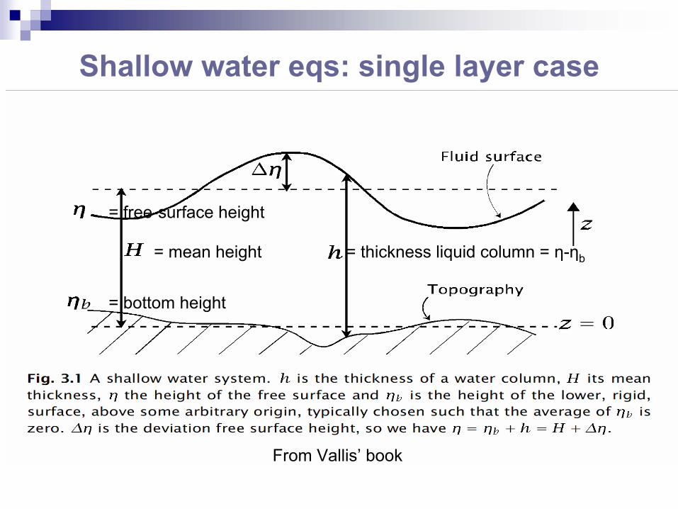
Shallow water eqs: single layer case

From Vallis’ book

= mean height = thickness liquid column = η-ηb

= free-surface height

= bottom height

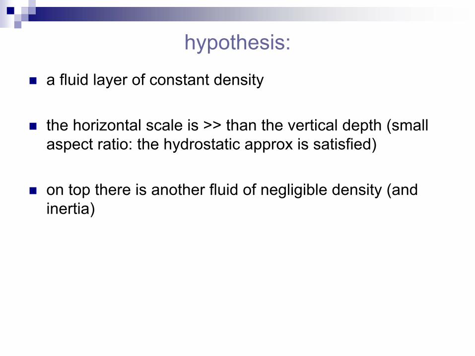
hypothesis:

a fluid layer of constant density

the horizontal scale is >> than the vertical depth (small aspect ratio: the hydrostatic approx is satisfied)

on top there is another fluid of negligible density (and inertia)

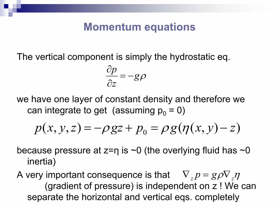
Momentum equations

The vertical component is simply the hydrostatic eq.

we have one layer of constant density and therefore we can integrate to get (assuming p0 = 0)

because pressure at z=η is ~0 (the overlying fluid has ~0 inertia)

A very important consequence is that (gradient of pressure) is independent on z ! We can

separate the horizontal and vertical eqs. completely

p gz

ρ∂= −

∂

0( , , ) ( ( , ) )p x y z gz p g x y zρ ρ η= − + = −

z zp gρ η∇ = ∇

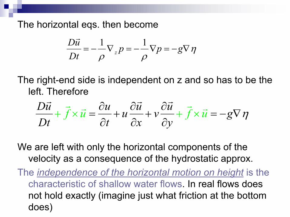
The horizontal eqs. then become

The right-end side is independent on z and so has to be the left. Therefore

We are left with only the horizontal components of the velocity as a consequence of the hydrostatic approx.

The independence of the horizontal motion on height is the characteristic of shallow water flows. In real flows does not hold exactly (imagine just what friction at the bottom does)

1 1z

Du p p gDt

ηρ ρ

= − ∇ = − ∇ = − ∇r

Du u u uu v gDt t x

f u f uy

η∂ ∂ ∂= + + =+ × + − ∇∂ ∂ ∂

×r r rr rr r

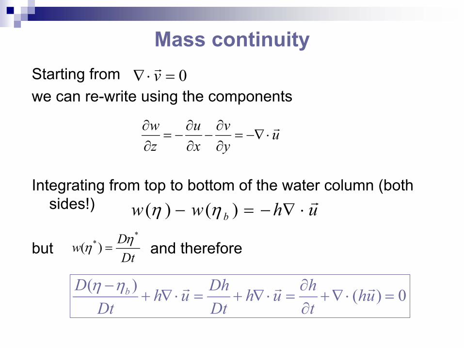
Starting from we can re-write using the components

Integrating from top to bottom of the water column (both sides!)

but and therefore

Mass continuity0v∇⋅ =

r

w u v uz x y

∂ ∂ ∂= − − = −∇⋅

∂ ∂ ∂r

( ) ( )bw w h uη η− = − ∇ ⋅r

**( ) Dw

Dtηη =

( ) ( ) 0bD Dh hh u h u huDt Dt tη η− ∂

+ ∇ ⋅ = + ∇ ⋅ = +∇ ⋅ =∂

r r r

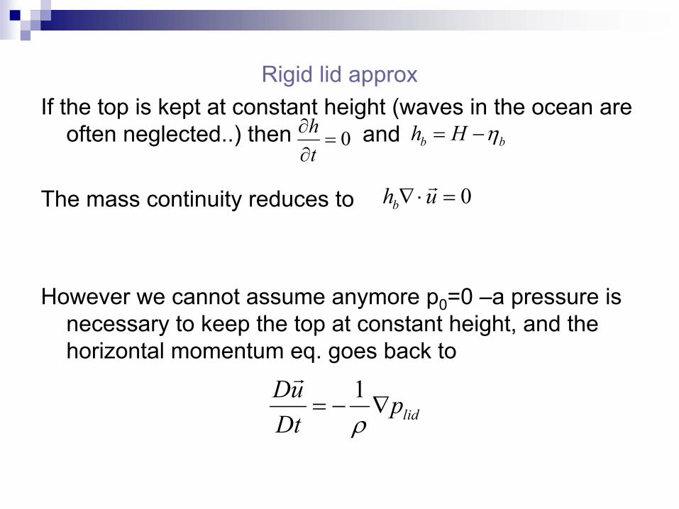
Rigid lid approxIf the top is kept at constant height (waves in the ocean are

often neglected..) then and

The mass continuity reduces to

However we cannot assume anymore p0=0 –a pressure is necessary to keep the top at constant height, and the horizontal momentum eq. goes back to

0ht

∂=

∂b bh H η= −

0bh u∇⋅ =r

1lid

Du pDt ρ

= − ∇r

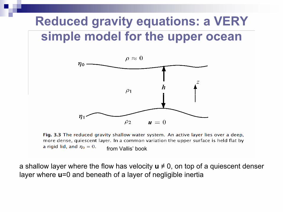
from Vallis’ book

a shallow layer where the flow has velocity u ≠ 0, on top of a quiescent denser layer where u=0 and beneath of a layer of negligible inertia

Reduced gravity equations: a VERY simple model for the upper ocean

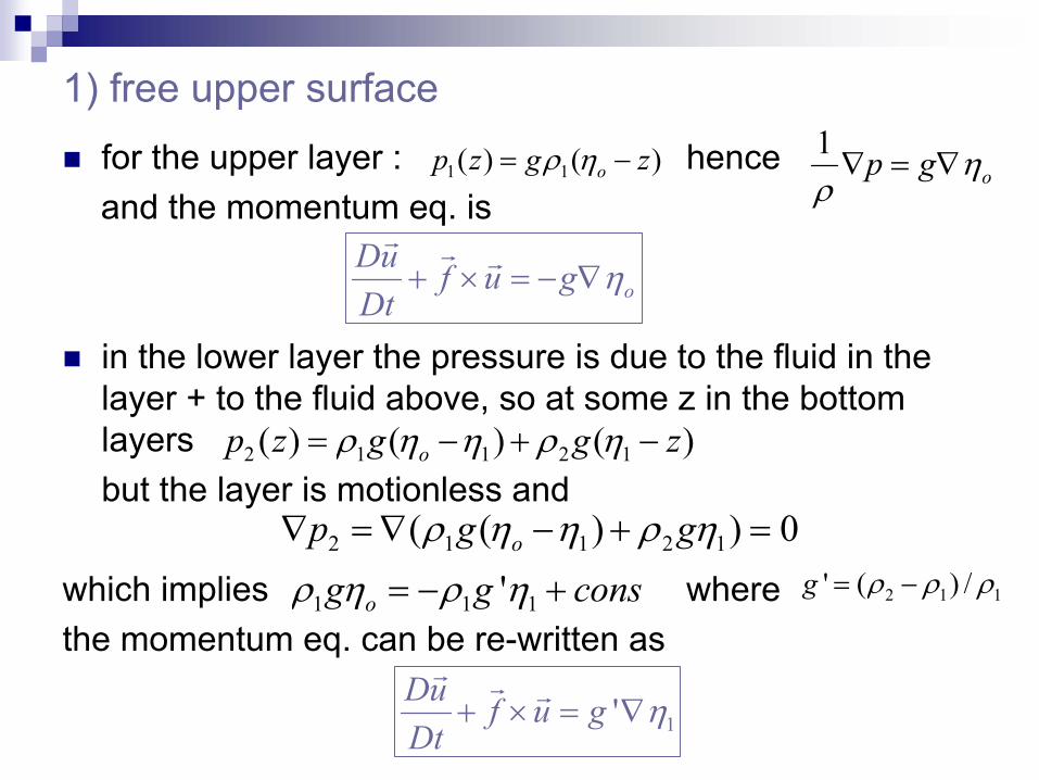
1) free upper surfacefor the upper layer : henceand the momentum eq. is

in the lower layer the pressure is due to the fluid in the layer + to the fluid above, so at some z in the bottom layers but the layer is motionless and

which implies wherethe momentum eq. can be re-written as

1 1( ) ( )op z g zρ η= − 1op g η

ρ∇ = ∇

oDu f u gDt

η+ × = − ∇r r r

2 1 1 2 1( ) ( ) ( )op z g g zρ η η ρ η= − + −

2 1 1 2 1( ( ) ) 0op g gρ η η ρ η∇ = ∇ − + =

1 1 1'og g consρ η ρ η= − + 2 1 1' ( ) /g ρ ρ ρ= −

1'Du f u gDt

η+ × = ∇r r r

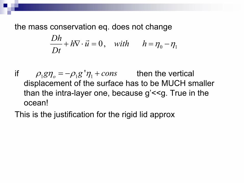
the mass conservation eq. does not change

if then the vertical displacement of the surface has to be MUCH smaller than the intra-layer one, because g’<<g. True in the ocean!

This is the justification for the rigid lid approx

0 10,Dh h u with hDt

η η+ ∇⋅ = = −r

1 1 1'og g consρ η ρ η= − +

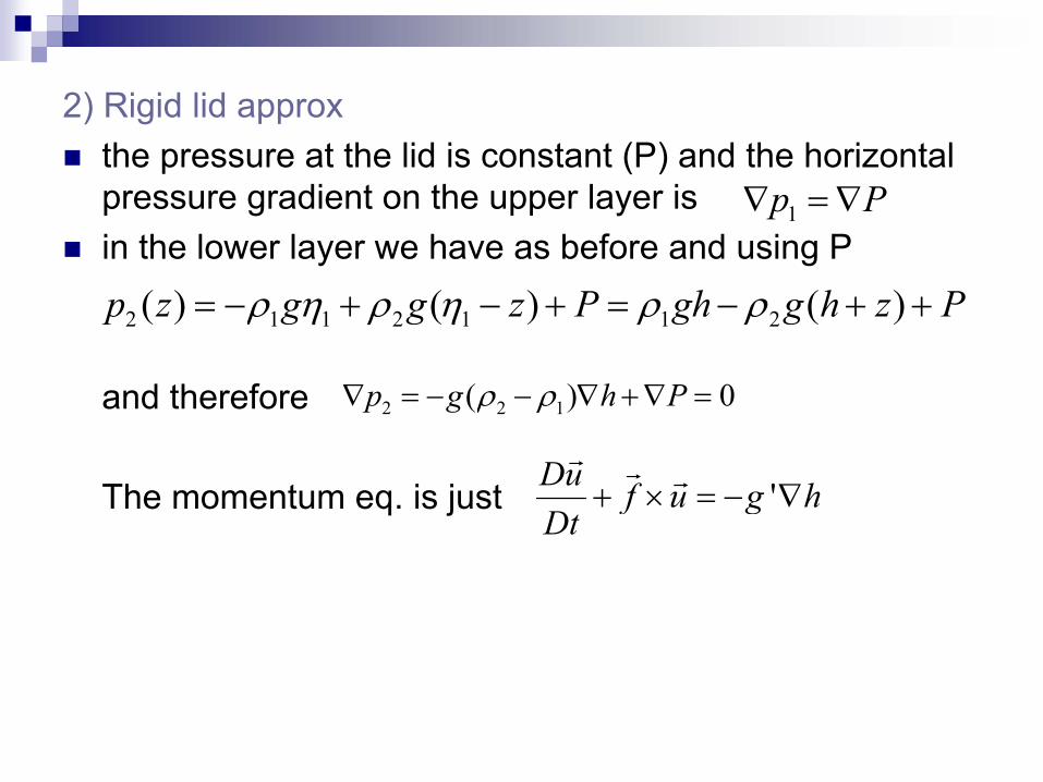
2) Rigid lid approxthe pressure at the lid is constant (P) and the horizontal pressure gradient on the upper layer is in the lower layer we have as before and using P

and therefore

The momentum eq. is just

1p P∇ =∇

2 1 1 2 1 1 2( ) ( ) ( )p z g g z P gh g h z Pρ η ρ η ρ ρ= − + − + = − + +

2 2 1( ) 0p g h Pρ ρ∇ = − − ∇ +∇ =

'Du f u g hDt

+ × = − ∇r r r

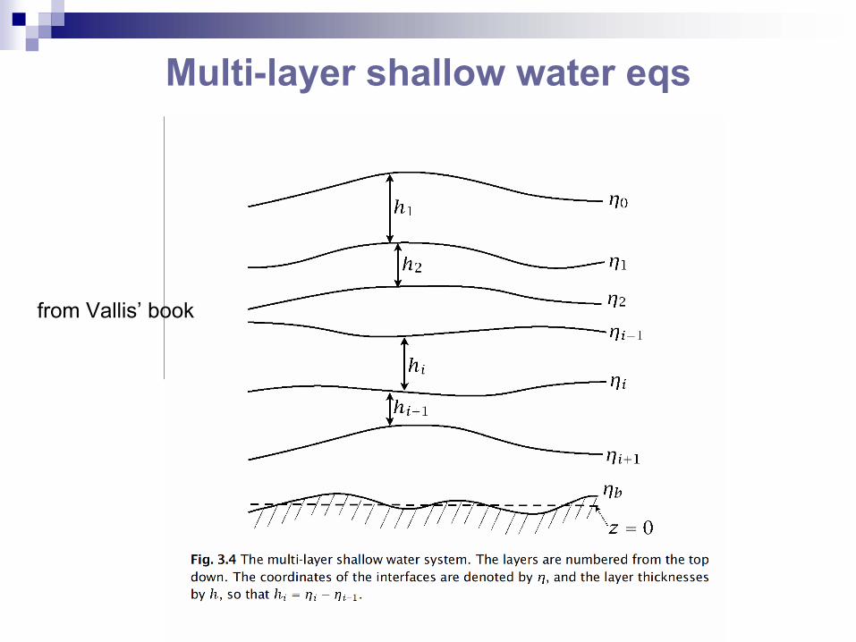
Multi-layer shallow water eqs

from Vallis’ book

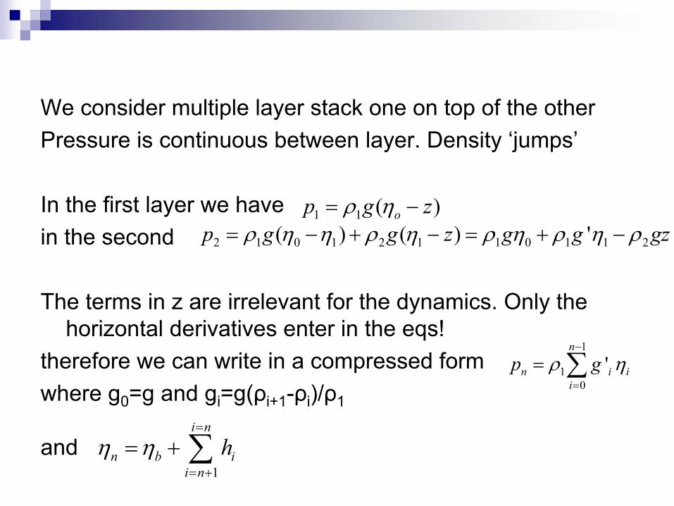
We consider multiple layer stack one on top of the otherPressure is continuous between layer. Density ‘jumps’

In the first layer we have in the second

The terms in z are irrelevant for the dynamics. Only the horizontal derivatives enter in the eqs!

therefore we can write in a compressed formwhere g0=g and gi=g(ρi+1-ρi)/ρ1

and

1 1 ( )op g zρ η= −2 1 0 1 2 1 1 0 1 1 2( ) ( ) 'p g g z g g gzρ η η ρ η ρ η ρ η ρ= − + − = + −

1

10'

n

n i ii

p gρ η−

=

= ∑

1

i n

n b ii n

hη η=

= +

= + ∑

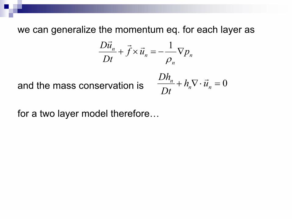
we can generalize the momentum eq. for each layer as

and the mass conservation is

for a two layer model therefore…

1nn n

n

Du f u pDt ρ

+ × = − ∇r r r

0nn n

Dh h uDt

+ ∇⋅ =r

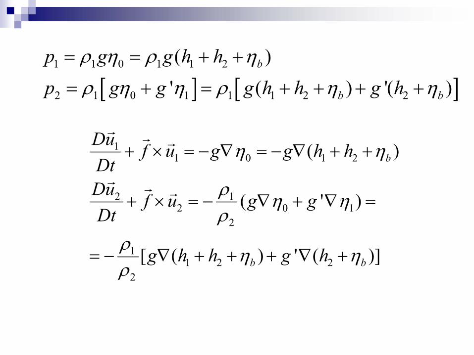
[ ] [ ]1 1 0 1 1 2

2 1 0 1 1 1 2 2

( )' ( ) '( )

b

b b

p g g h hp g g g h h g h

ρ η ρ η

ρ η η ρ η η

= = + +

= + = + + + +

11 0 1 2

2 12 0 1

2

11 2 2

2

( )

( ' )

[ ( ) ' ( )]

b

b b

Du f u g g h hDtDu f u g gDt

g h h g h

η η

ρ η ηρ

ρ η ηρ

+ × = − ∇ = − ∇ + +

+ × = − ∇ + ∇ =

= − ∇ + + + ∇ +

r r r

r r r

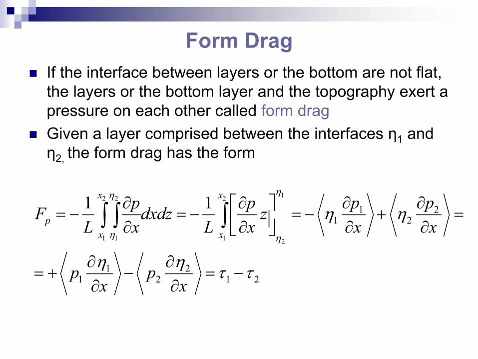
Form DragIf the interface between layers or the bottom are not flat, the layers or the bottom layer and the topography exert a pressure on each other called form dragGiven a layer comprised between the interfaces η1 and η2, the form drag has the form

12 2 2

1 1 1 2

1 21 2

1 21 2 1 2

1 1x x

px x

p pp pF dxdz zL x L x x x

p px x

ηη

η η

η η

η η τ τ

∂ ∂∂ ∂ = − = − = − + = ∂ ∂ ∂ ∂

∂ ∂= + − = −

∂ ∂

∫ ∫ ∫

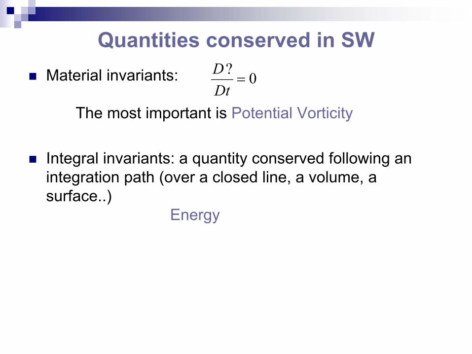
Quantities conserved in SWMaterial invariants:

The most important is Potential Vorticity

Integral invariants: a quantity conserved following an integration path (over a closed line, a volume, a surface..)

Energy

? 0DDt

=

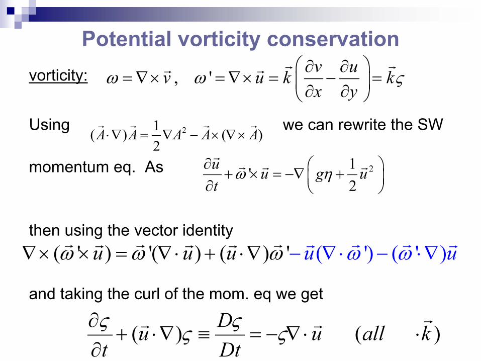
Potential vorticity conservationvorticity:

Using we can rewrite the SW

momentum eq. As

then using the vector identity

and taking the curl of the mom. eq we get

, ' v uv u k kx y

ω ω ς ∂ ∂

= ∇× = ∇× = − = ∂ ∂

r rr r

21( ) ( )2

A A A A A⋅∇ = ∇ − × ∇×r r r r

21'2

u u g ut

ω η∂ + × = −∇ + ∂

rr r r

( ' ) '( ( ') ( ') ) )( 'u u u u uω ωω ω ω∇× × = ∇⋅ + ⋅∇ − ∇ ⋅ − ⋅∇r rr rr r rr rr

( ) ( )Du u all kt Dtς ςς ς∂+ ⋅∇ ≡ = − ∇⋅ ⋅

∂

rr r

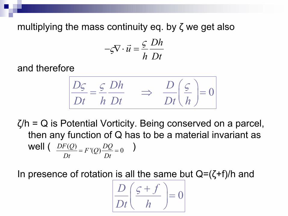
multiplying the mass continuity eq. by ζ we get also

and therefore

ζ/h = Q is Potential Vorticity. Being conserved on a parcel, then any function of Q has to be a material invariant as well ( )

In presence of rotation is all the same but Q=(ζ+f)/h and

Dhuh Dtςς− ∇ ⋅ =

r

0D Dh DDt h Dt Dt hς ς ς = ⇒ =

( ) '( ) 0DF Q DQF QDt Dt

= =

0D fDt h

ς + =

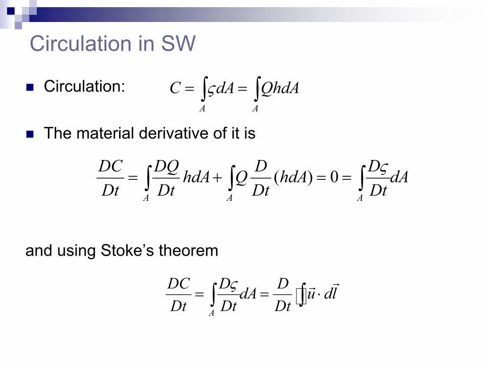
Circulation in SW

Circulation:

The material derivative of it is

and using Stoke’s theorem

A A

C dA QhdAς= =∫ ∫

( ) 0A A A

DC DQ D DhdA Q hdA dADt Dt Dt Dt

ς= + = =∫ ∫ ∫

A

DC D DdA u dlDt Dt Dt

ς= = ⋅∫ ∫

rr

Conservation of energy in SWEnergy is conserved BEFORE we make simplifications and assumptions. In SW is still an integral invariant

The kinetic energy per unit area is

The potential (due to gravity) is

In the assumption of a flat bottom, let’s look for the evolution of PE:

212 ohuρ r

2

0

12

h

o oPE gzdz ghρ ρ= =∫

2 2 2 22 0

2 2 2 2D gh gh gh ghgh u u uDt t

∂+ ∇ ⋅ = = +∇ ⋅ + ∇ ⋅ ∂

r r r

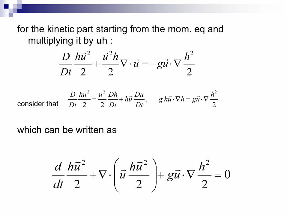
for the kinetic part starting from the mom. eq and multiplying it by uh :

consider that

which can be written as

2 2 2

2 2 2D hu u h hu guDt

+ ∇⋅ = − ⋅∇r r

r r

2 2 2

,2 2 2

D hu u Dh Du hhu g hu h guDt Dt Dt

= + ⋅∇ = ⋅∇r r r

r r r

0222

222

=∇⋅+

⋅∇+

huguhuuhdtd r

rr

r

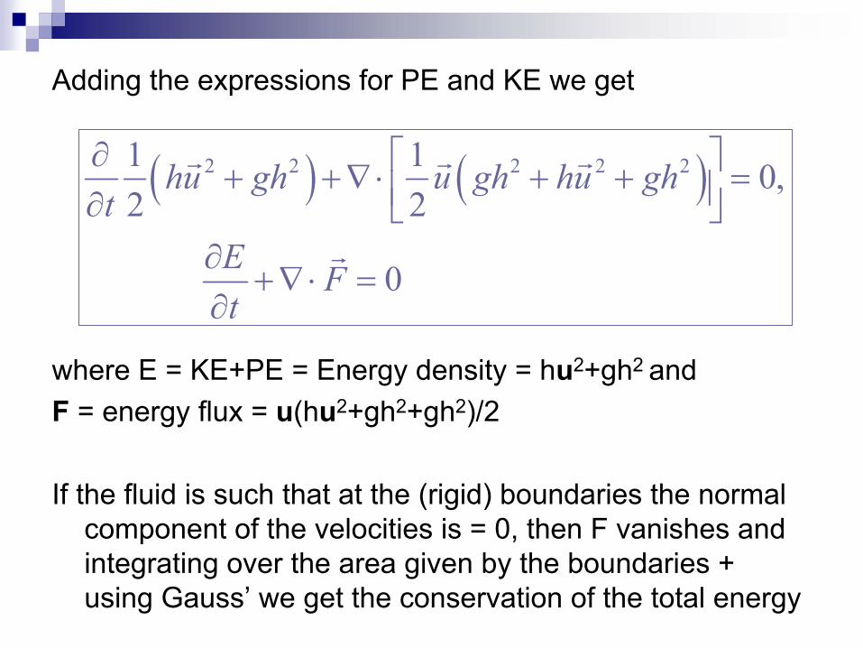
Adding the expressions for PE and KE we get

where E = KE+PE = Energy density = hu2+gh2 andF = energy flux = u(hu2+gh2+gh2)/2

If the fluid is such that at the (rigid) boundaries the normal component of the velocities is = 0, then F vanishes and integrating over the area given by the boundaries + using Gauss’ we get the conservation of the total energy

( ) ( )2 2 2 2 21 1 0,2 2

0

hu gh u gh hu ght

E Ft

∂ + +∇ ⋅ + + = ∂ ∂

+∇ ⋅ =∂

r r r

r

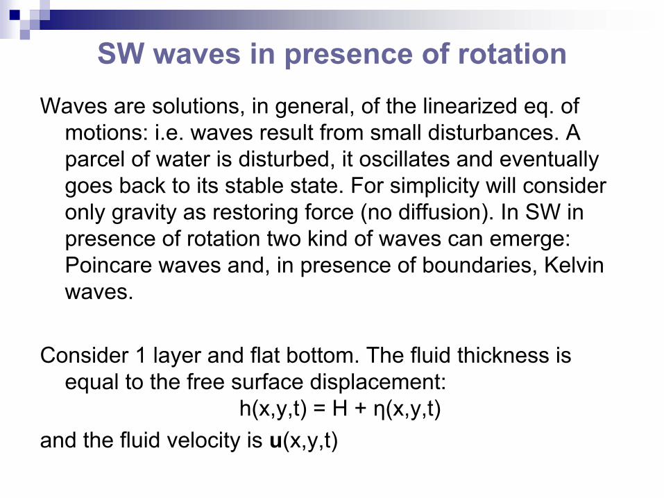
SW waves in presence of rotationWaves are solutions, in general, of the linearized eq. of

motions: i.e. waves result from small disturbances. A parcel of water is disturbed, it oscillates and eventually goes back to its stable state. For simplicity will consider only gravity as restoring force (no diffusion). In SW in presence of rotation two kind of waves can emerge: Poincare waves and, in presence of boundaries, Kelvin waves.

Consider 1 layer and flat bottom. The fluid thickness is equal to the free surface displacement:

h(x,y,t) = H + η(x,y,t)and the fluid velocity is u(x,y,t)

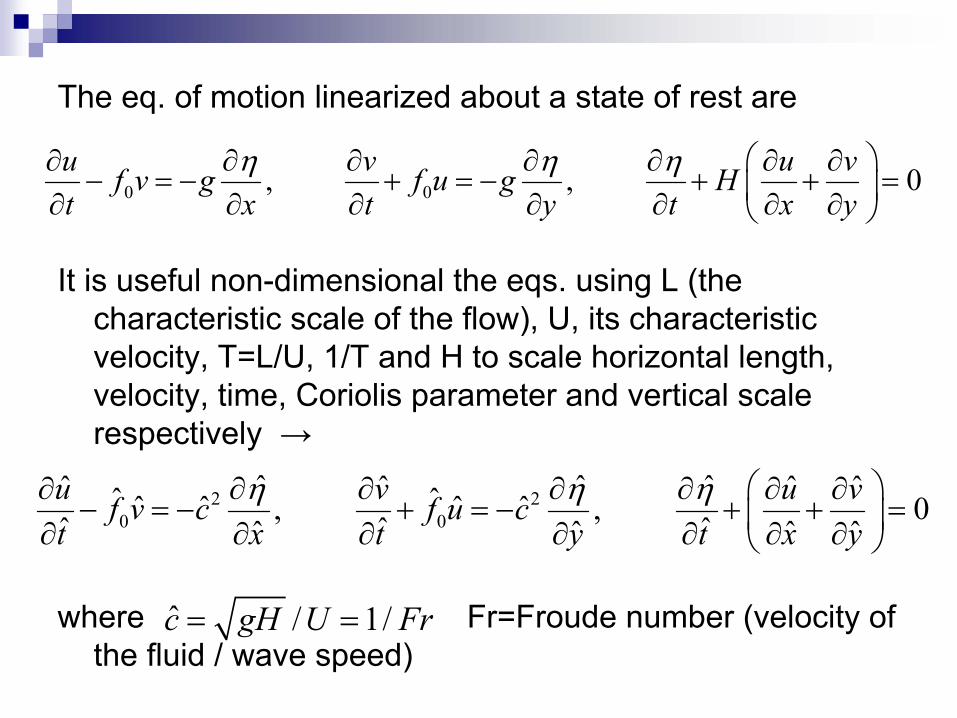
The eq. of motion linearized about a state of rest are

It is useful non-dimensional the eqs. using L (the characteristic scale of the flow), U, its characteristic velocity, T=L/U, 1/T and H to scale horizontal length, velocity, time, Coriolis parameter and vertical scale respectively →

where Fr=Froude number (velocity of the fluid / wave speed)

0 0, , 0u v u vf v g f u g Ht x t y t x y

η η η ∂ ∂ ∂ ∂ ∂ ∂ ∂− = − + = − + + = ∂ ∂ ∂ ∂ ∂ ∂ ∂

2 20 0

ˆ ˆ ˆˆ ˆ ˆ ˆˆ ˆˆ ˆ ˆ ˆ, , 0ˆ ˆ ˆˆ ˆ ˆ ˆu v u vf v c f u ct x t y t x y

η η η ∂ ∂ ∂ ∂ ∂ ∂ ∂− = − + = − + + = ∂ ∂ ∂ ∂ ∂ ∂ ∂

ˆ / 1/c gH U Fr= =

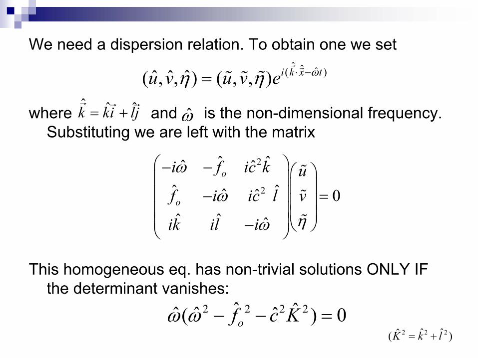
We need a dispersion relation. To obtain one we set

where and is the non-dimensional frequency. Substituting we are left with the matrix

This homogeneous eq. has non-trivial solutions ONLY IF the determinant vanishes:

ˆ ˆ ˆ( )ˆˆ ˆ( , , ) ( , , ) i k x tu v u v e ωη η ⋅ −=r r

%% %

ˆ ˆ ˆk ki lj= +r r r

ω̂

2

2

ˆ ˆˆ ˆˆ ˆˆ ˆ 0ˆ ˆ ˆ

o

o

i f ic k uf i ic l v

ik il i

ω

ωηω

− − − = −

%

%

%

2 2 2 2ˆ ˆˆ ˆ ˆ( ) 0of c Kω ω − − =2 2 2ˆ ˆˆ( )K k l= +

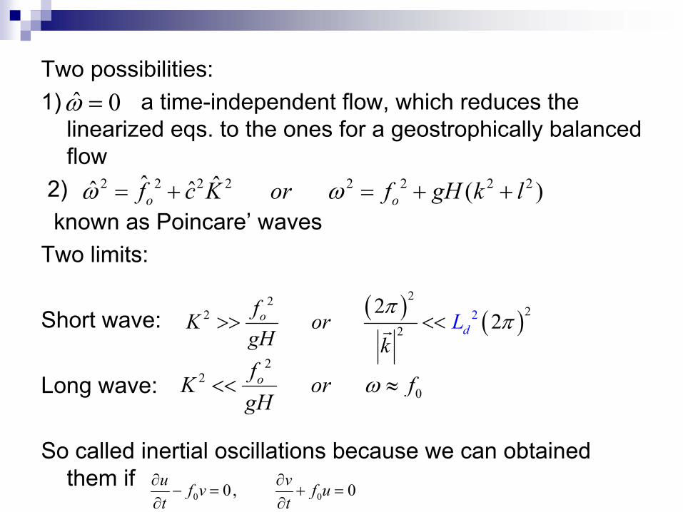
Two possibilities:1) a time-independent flow, which reduces the

linearized eqs. to the ones for a geostrophically balanced flow

2)known as Poincare’ waves

Two limits:

Short wave:

Long wave:

So called inertial oscillations because we can obtained them if

ˆ 0ω =

2 2 2 2 2 2 2 2ˆ ˆˆ ˆ ( )o of c K or f gH k lω ω= + = + +

( ) ( )22

22

22 22d

ofK or LgH k

ππ>> <<r

22

0ofK or fgH

ω<< ≈

0 00, 0u vf v f ut t

∂ ∂− = + =

∂ ∂

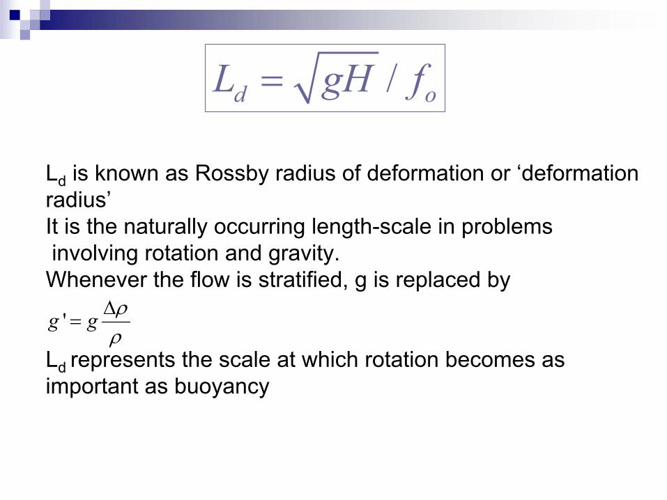
/d oL gH f=

Ld is known as Rossby radius of deformation or ‘deformation radius’It is the naturally occurring length-scale in problemsinvolving rotation and gravity. Whenever the flow is stratified, g is replaced by

Ld represents the scale at which rotation becomes as important as buoyancy

'g g ρρ∆

=

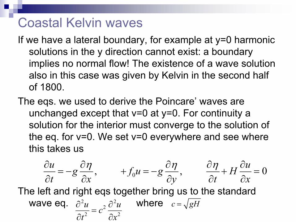
Coastal Kelvin wavesIf we have a lateral boundary, for example at y=0 harmonic

solutions in the y direction cannot exist: a boundary implies no normal flow! The existence of a wave solution also in this case was given by Kelvin in the second half of 1800.

The eqs. we used to derive the Poincare’ waves are unchanged except that v=0 at y=0. For continuity a solution for the interior must converge to the solution of the eq. for v=0. We set v=0 everywhere and see where this takes us

The left and right eqs together bring us to the standard wave eq. where

0, , 0u ug f u g Ht x y t x

η η η∂ ∂ ∂ ∂ ∂= − + = − + =

∂ ∂ ∂ ∂ ∂

2 22

2 2

u uct x

∂ ∂=

∂ ∂c gH=

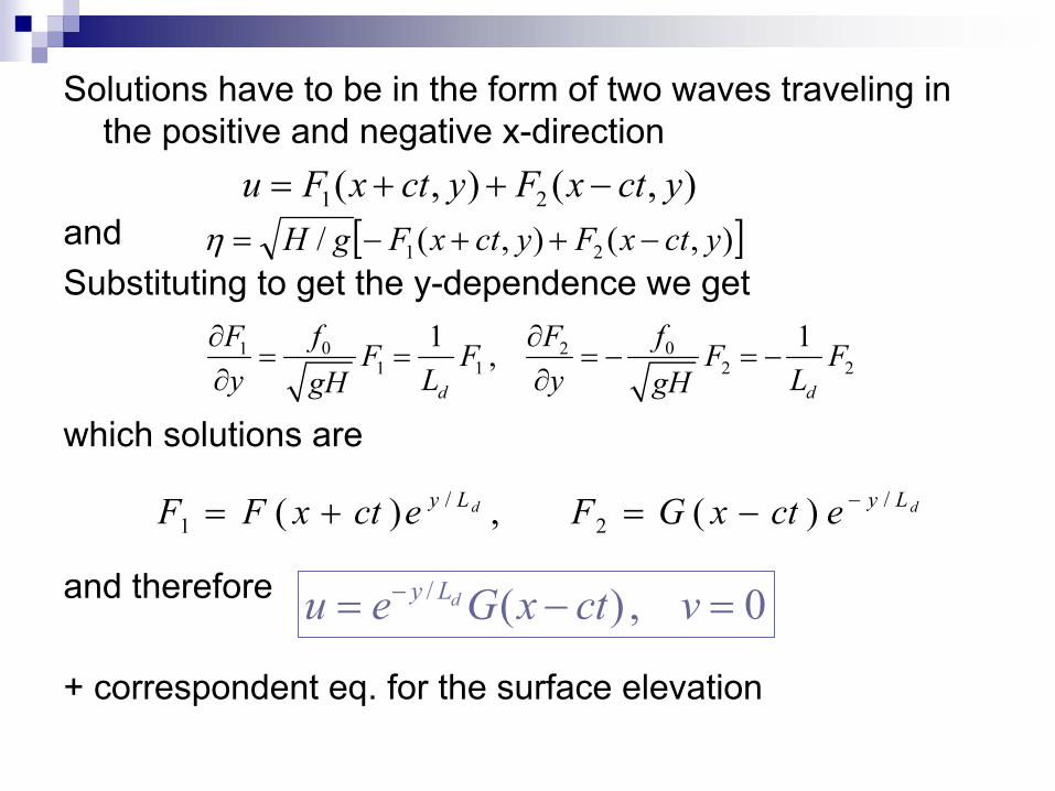
Solutions have to be in the form of two waves traveling in the positive and negative x-direction

and Substituting to get the y-dependence we get

which solutions are

and therefore

+ correspondent eq. for the surface elevation

1 2( , ) ( , )u F x ct y F x ct y= + + −

0 01 21 1 2 2

1 1,d d

f fF FF F F Fy L y LgH gH

∂ ∂= = = − = −

∂ ∂

/ ( ) , 0dy Lu e G x ct v−= − =

[ ]),(),(/ 21 yctxFyctxFgH −++−=η

dd LyLy ectxGFectxFF /2

/1 )(,)( −−=+=

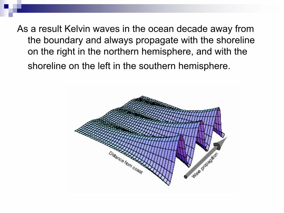
As a result Kelvin waves in the ocean decade away from the boundary and always propagate with the shoreline on the right in the northern hemisphere, and with the shoreline on the left in the southern hemisphere.

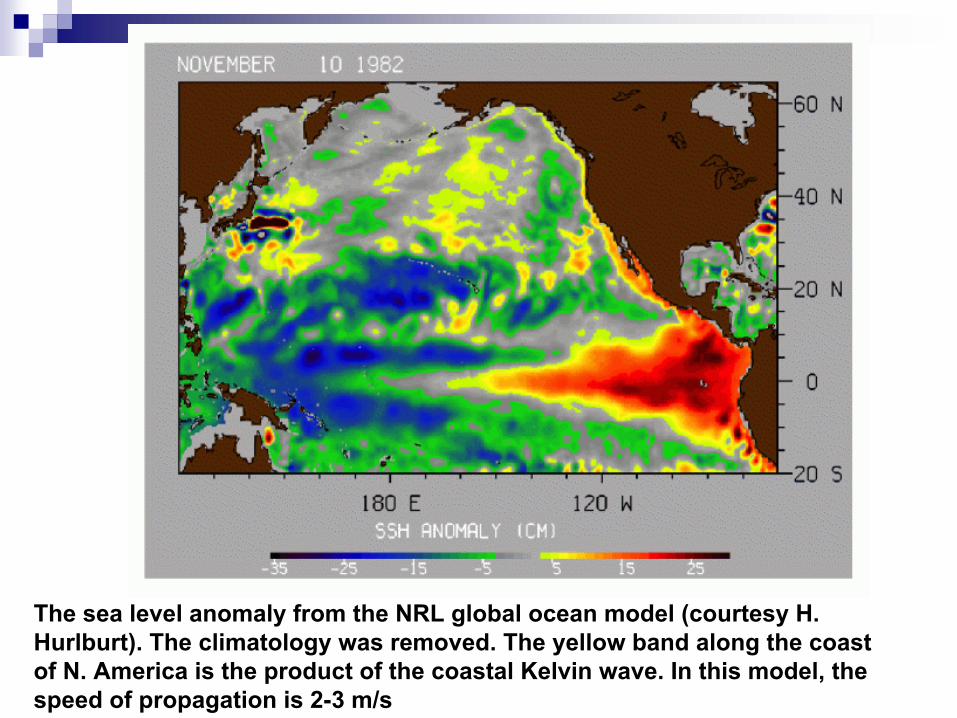
The sea level anomaly from the NRL global ocean model (courtesy H. Hurlburt). The climatology was removed. The yellow band along the coast of N. America is the product of the coastal Kelvin wave. In this model, the speed of propagation is 2-3 m/s

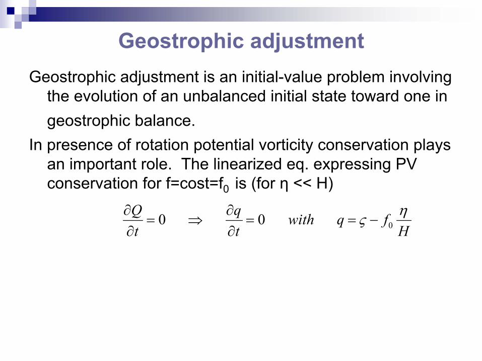
Geostrophic adjustmentGeostrophic adjustment is an initial-value problem involving

the evolution of an unbalanced initial state toward one in geostrophic balance.

In presence of rotation potential vorticity conservation plays an important role. The linearized eq. expressing PV conservation for f=cost=f0 is (for η << H)

00 0Q q with q ft t H

ης∂ ∂= ⇒ = = −

∂ ∂

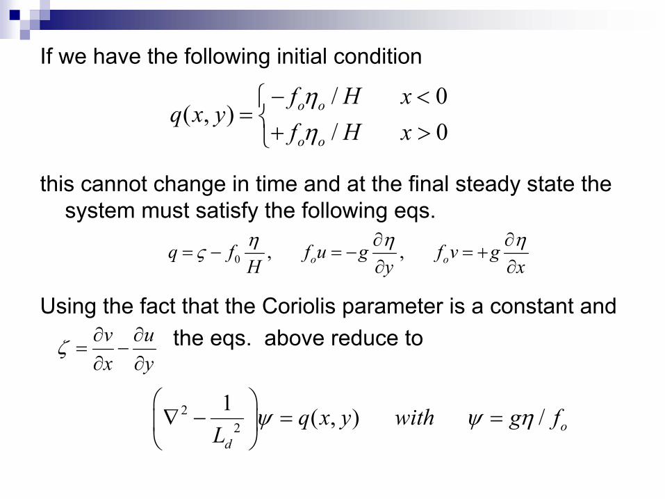
If we have the following initial condition

this cannot change in time and at the final steady state the system must satisfy the following eqs.

Using the fact that the Coriolis parameter is a constant and the eqs. above reduce to

/ 0( , )

/ 0o o

o o

f H xq x y

f H xηη

− <= + >

v ux y

ζ ∂ ∂= −∂ ∂

0 , ,o oq f f u g f v gH y xη η ης ∂ ∂

= − = − = +∂ ∂

22

1 ( , ) / od

q x y with g fL

ψ ψ η ∇ − = =

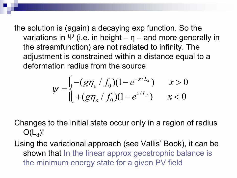
the solution is (again) a decaying exp function. So the variations in Ψ (i.e. in height – η – and more generally in the streamfunction) are not radiated to infinity. The adjustment is constrained within a distance equal to a deformation radius from the source

Changes to the initial state occur only in a region of radius O(Ld)!

Using the variational approach (see Vallis’ Book), it can be shown that In the linear approx geostrophic balance is the minimum energy state for a given PV field

/0

/0

( / )(1 ) 0( / )(1 ) 0

d

d

x Lo

x Lo

g f e xg f e xη

ψη

−− − >= + − <

For a generic (and nice) derivation check http://snowball.millersville.edu/~adecaria/ESCI343/esci343_lesson17_geostrophic_adjustment.html

Further reading: Gill, A. E., 1982: Atmosphere-Ocean Dynamics. Academic Press, New York, 662 pp.

Check those web site: http://meted.ucar.edu/nwp/pcu1/d_adjust/1_0.htmand http://www.atmos.washington.edu/~lharris/adjust.html

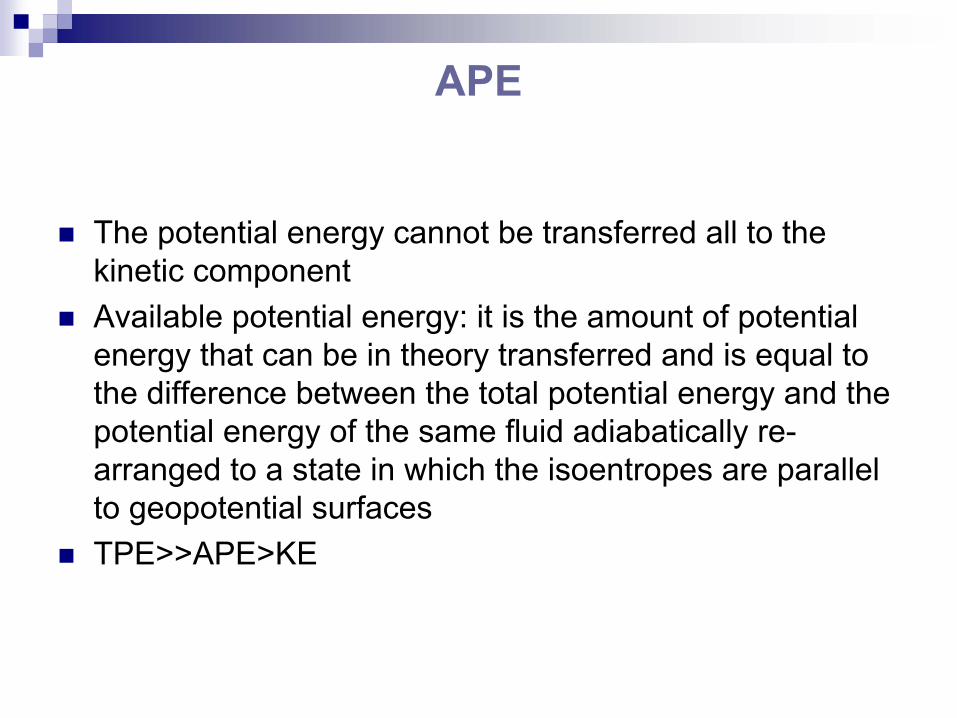
APE

The potential energy cannot be transferred all to the kinetic componentAvailable potential energy: it is the amount of potential energy that can be in theory transferred and is equal to the difference between the total potential energy and the potential energy of the same fluid adiabatically re-arranged to a state in which the isoentropes are parallel to geopotential surfacesTPE>>APE>KE

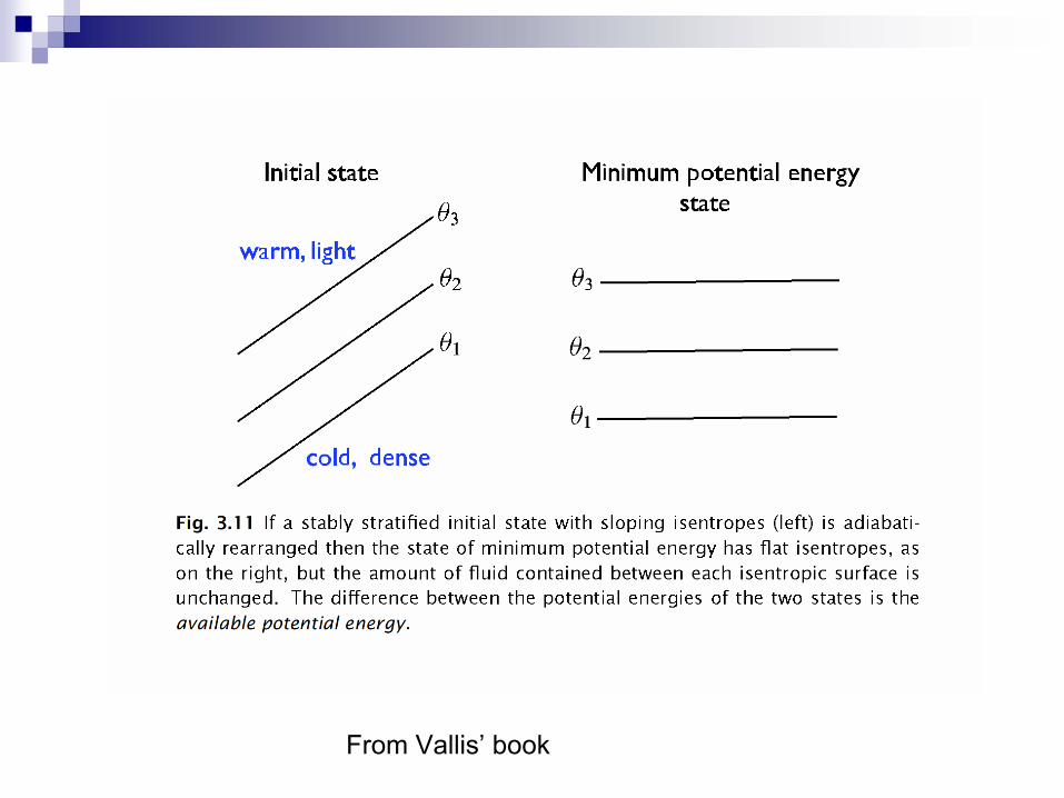
From Vallis’ book