LinearAlgebra - SHUYOU YU
21
Robust Control v3.2, 20133 Linear Algebra 21 • Linear subspaces • Eigenvalues and Eigenvectors • Matrix inversion formulas • Invariant subspaces • Vector norms and matrix norms
Transcript of LinearAlgebra - SHUYOU YU
Robust Control ������������
��
�����������
v3.2, 2013�3��
��������� Linear Algebra
21
• Linear subspaces
• Eigenvalues and Eigenvectors
• Matrix inversion formulas
• Invariant subspaces
• Vector norms and matrix norms
��������� Linear Algebra
22
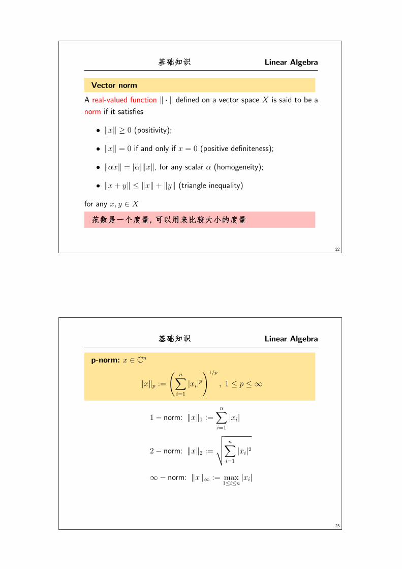
Vector norm
A real-valued function ‖ · ‖ defined on a vector space X is said to be a
norm if it satisfies
• ‖x‖ ≥ 0 (positivity);
• ‖x‖ = 0 if and only if x = 0 (positive definiteness);
• ‖αx‖ = |α|‖x‖, for any scalar α (homogeneity);
• ‖x+ y‖ ≤ ‖x‖+ ‖y‖ (triangle inequality)
for any x, y ∈ X
��������� ���������, ���������������������������������
��������� Linear Algebra
23
p-norm: x ∈ Cn
‖x‖p :=(
n∑i=1
|xi|p)1/p
, 1 ≤ p ≤ ∞
1− norm: ‖x‖1 :=n∑
i=1
|xi|
2− norm: ‖x‖2 :=√√√√ n∑
i=1
|xi|2
∞− norm: ‖x‖∞ := max1≤i≤n
|xi|
��������� Linear Algebra
24
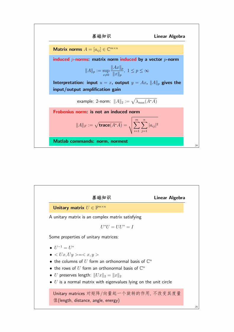
Matrix norms A = [aij] ∈ Cm×n
induced p-norms: matrix norm induced by a vector p-norm
‖A‖p := supx �=0
‖Ax‖p‖x‖p , 1 ≤ p ≤ ∞
Interpretation: input u = x, output y = Ax, ‖A‖p gives the
input/output amplification gain
example: 2-norm: ‖A‖2 :=√
λmax(A∗A)
Frobenius norm: is not an induced norm
‖A‖F :=√
trace(A∗A) =
√√√√ m∑i=1
n∑j=1
|aij|2
Matlab commands: norm, normest
��������� Linear Algebra
25
Unitary matrix U ∈ Fm×n
A unitary matrix is an complex matrix satisfying
U∗U = UU∗ = I
Some properties of unitary matrices:
• U−1 = U∗
• < Ux, Uy >=< x, y >
• the columns of U form an orthonormal basis of Cn
• the rows of U form an orthonormal basis of Cn
• U preserves length: ‖Ux‖2 = ‖x‖2• U is a normal matrix with eigenvalues lying on the unit circle
Unitary matrices ���/��� ������, ������
�(length, distance, angle, energy)
��������� Linear Algebra
26
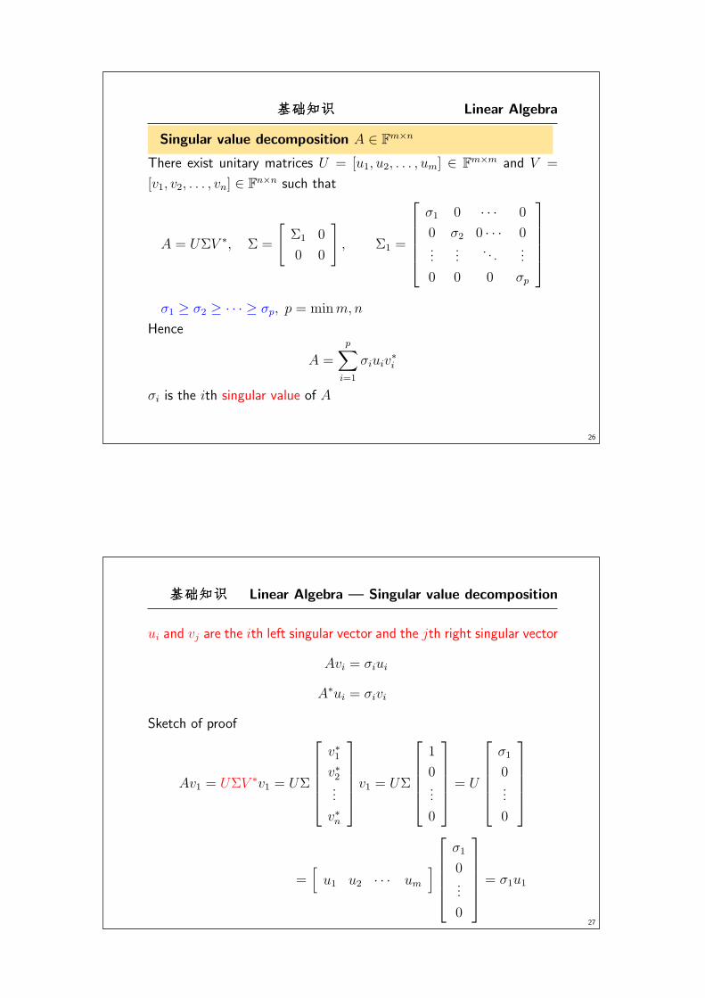
Singular value decomposition A ∈ Fm×n
There exist unitary matrices U = [u1, u2, . . . , um] ∈ Fm×m and V =
[v1, v2, . . . , vn] ∈ Fn×n such that
A = UΣV ∗, Σ =
[Σ1 0
0 0
], Σ1 =
⎡⎢⎢⎢⎢⎣
σ1 0 · · · 0
0 σ2 0 · · · 0...
.... . .
...
0 0 0 σp
⎤⎥⎥⎥⎥⎦
σ1 ≥ σ2 ≥ · · · ≥ σp, p = minm,n
Hence
A =
p∑i=1
σiuiv∗i
σi is the ith singular value of A
��������� Linear Algebra — Singular value decomposition
27
ui and vj are the ith left singular vector and the jth right singular vector
Avi = σiui
A∗ui = σivi
Sketch of proof
Av1 = UΣV ∗v1 = UΣ
⎡⎢⎢⎢⎢⎣
v∗1v∗2...
v∗n
⎤⎥⎥⎥⎥⎦ v1 = UΣ
⎡⎢⎢⎢⎢⎣
1
0...
0
⎤⎥⎥⎥⎥⎦ = U
⎡⎢⎢⎢⎢⎣
σ1
0...
0
⎤⎥⎥⎥⎥⎦
=[u1 u2 · · · um
]⎡⎢⎢⎢⎢⎣
σ1
0...
0
⎤⎥⎥⎥⎥⎦ = σ1u1
��������� Linear Algebra — Singular value decomposition
28
σ2i is an eigenvalue of AA∗ or A∗A
A = UΣV ∗, AA∗ = UΣV ∗V ΣU∗ = UΣ2U∗
eig(AA∗) = eig(UΣ2U∗) = {σ21, σ
22, · · · , σ2
p}ui is an eigenvector of AA∗ and vi is an eigenvector of A∗A
A∗Avi = A∗σiui = σiA∗ui = σ2
i vi
AA∗ui = Aσivi = σiAvi = σ2i ui
the largest singular value of A: σ(A) = σmax(A) = σ1
the smallest singular value of A: σ(A) = σmin(A) = σp
If define y = Ax =⇒ an interpretation of singular values
��������� Linear Algebra — Singular value decomposition
29
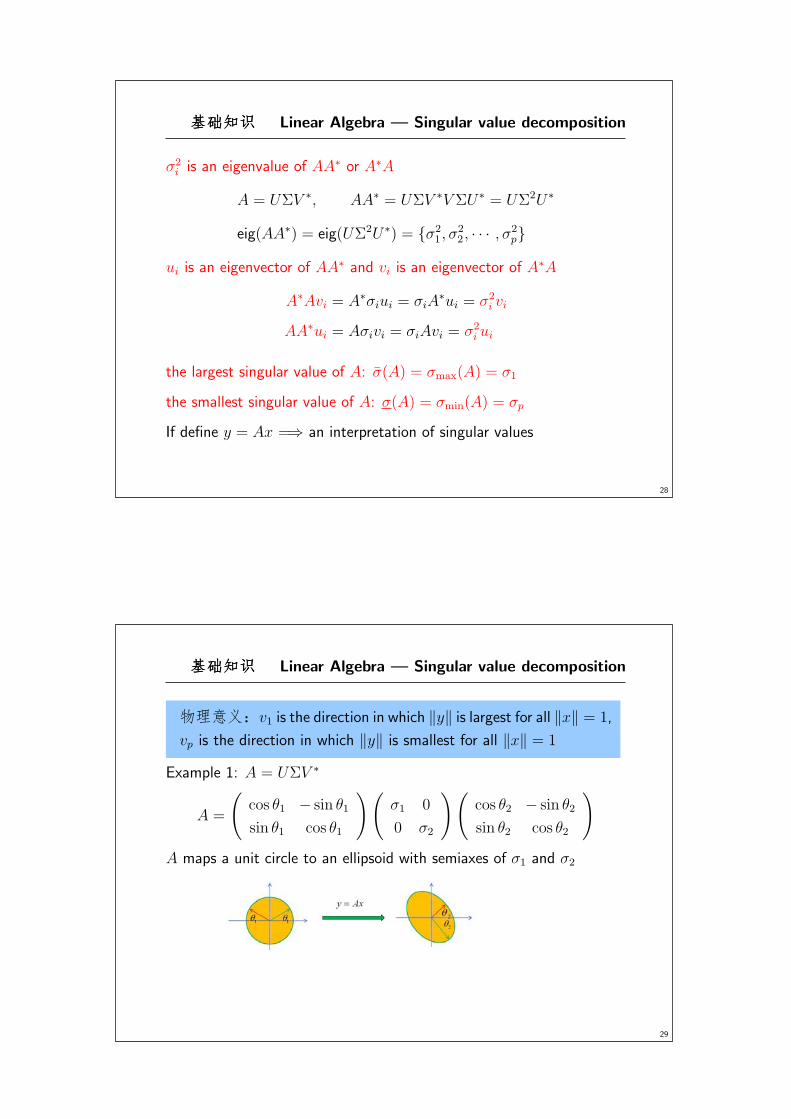
��v1 is the direction in which ‖y‖ is largest for all ‖x‖ = 1,
vp is the direction in which ‖y‖ is smallest for all ‖x‖ = 1
Example 1: A = UΣV ∗
A =
(cos θ1 − sin θ1
sin θ1 cos θ1
)(σ1 0
0 σ2
)(cos θ2 − sin θ2
sin θ2 cos θ2
)
A maps a unit circle to an ellipsoid with semiaxes of σ1 and σ2
��������� Linear Algebra — Singular value decomposition
30
��������:
����: v1 is the highest gain input (control) direction, vp is
the lowest gain input direction Av1 = σ1u1, Avp = σpup
��: u1 is the highest gain output (observing) direction, up
is the lowest gain output direction A∗u1 = σ1v1, A∗up = σpvp
σ(A) := max‖x‖=1
‖Ax‖ = maxx �=0
‖Ax‖‖x‖
σ(A) := min‖x‖=1
‖Ax‖ = minx�=0
‖Ax‖‖x‖
��������� Linear Algebra — Singular value decomposition
31
Example 2: ���� A ∈ Rm×n �� ����������
A = UΣV ∗, Σ =
[Σ1 0
0 0
],
Σ1 = diag(
σ1 · · · σl σl+1 · · · σp,), σl+1 � σl
Σ1 ∈ Rl×l ���������=⇒ ��
Example 3: Model reduction A ∈ Fm×n ������
������ Linear Systems – ������������
32
[x
y
]=
[A B
C D
][x
u
]
Controllability: The dynamical system or the pair (A,B) is
said to be controllable if, for any initial state x(0) = x0, t1 > 0
and final state x1, there exists a (piecewise continuous) input
u(·) such that the solution of the system satisfies x(t1) = x1.
(A,B) ��������������������������� F ������������ A + BF ������
���
Stabilizability: A ������������������������������
(A,B) ��������������������� F ������ A+BF ������������
��������� Linear Systems – ���������
33
[x
y
]=
[A B
C D
][x
u
]
Observability: The dynamical system or the pair (C,A) is
said to be observable if, for any t1 > 0, the initial state
x(0) = x0 can be determined from the time history of the
input u(t) and the output y(t) in the interval [0, t1].
(C,A) ��������������������� L ������ A+LC ������������
Detectability: A ���������������������������
(C,A) ������������������ L ������ A+ LC ������������
��������� Linear Systems: Pole-Zero Cancelation
34
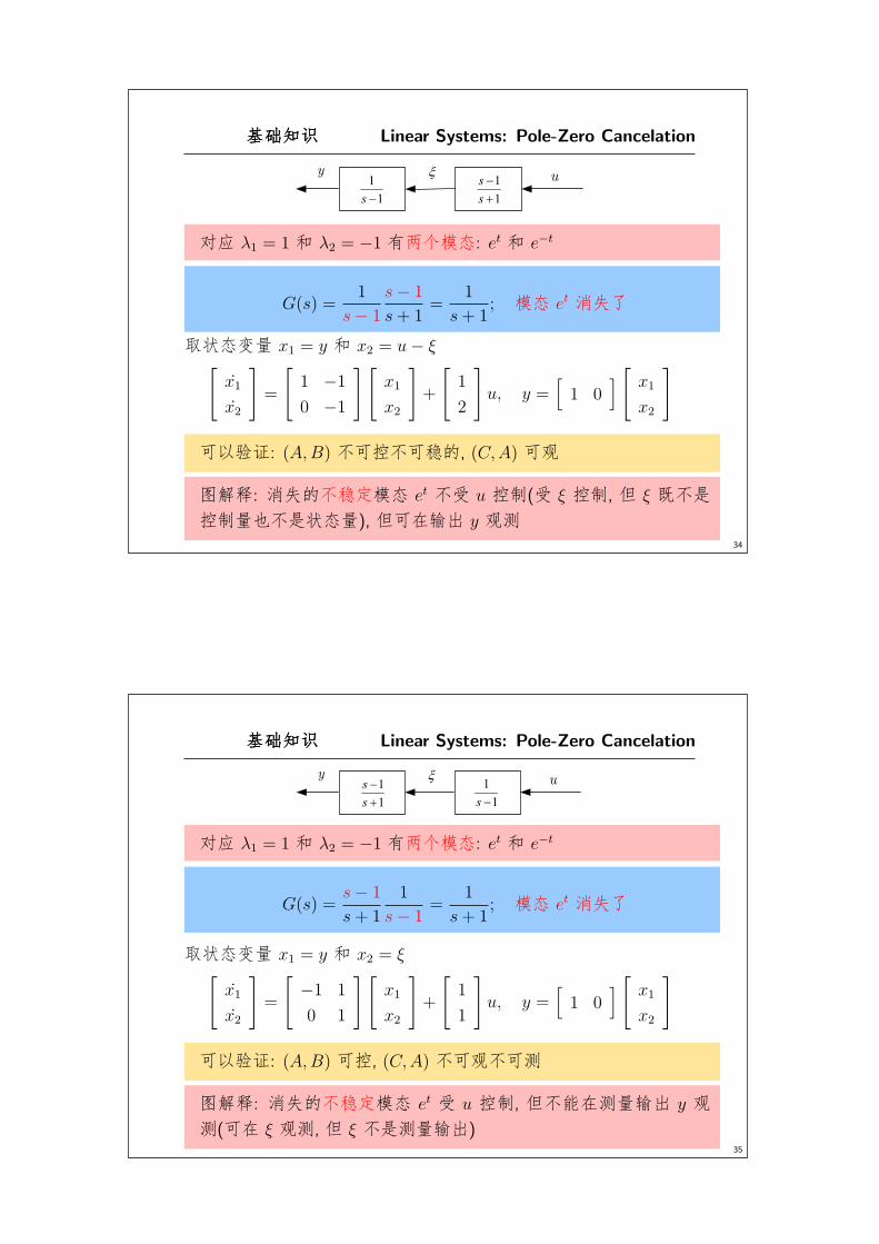
y u11s
11
ss
�� λ1 = 1 � λ2 = −1 �����: et � e−t
G(s) =1
s− 1
s− 1
s+ 1=
1
s+ 1; �� et ��
����� x1 = y � x2 = u− ξ[x1
x2
]=
[1 −1
0 −1
][x1
x2
]+
[1
2
]u, y =
[1 0
] [ x1
x2
]
����: (A,B) �������, (C,A) ��
���: ������ et � u ��( ξ ��, � ξ ���
���������), ����� y ��
��������� Linear Systems: Pole-Zero Cancelation
35
y u11s
11
ss
�� λ1 = 1 λ2 = −1 ����: et e−t
G(s) =s− 1
s+ 1
1
s− 1=
1
s+ 1; �� et �
����� x1 = y x2 = ξ[x1
x2
]=
[−1 1
0 1
][x1
x2
]+
[1
1
]u, y =
[1 0
] [ x1
x2
]
����: (A,B) ��, (C,A) ������
���: ������ et � u ��, �������� y �
�(�� ξ ��, � ξ ������)
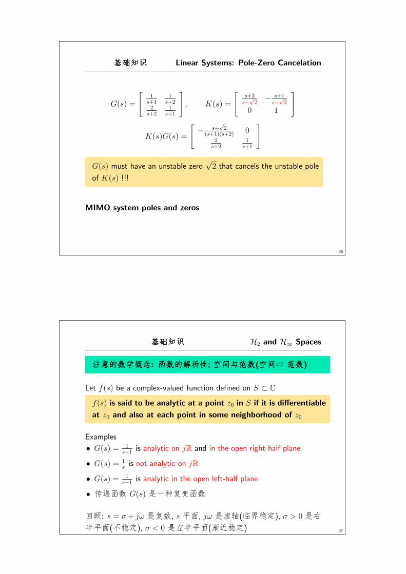
��������� Linear Systems: Pole-Zero Cancelation
36
G(s) =
[1
s+11
s+22
s+21
s+1
], K(s) =
[s+2s−√
2− s+1
s−√2
0 1
]
K(s)G(s) =
[− s+
√2
(s+1)(s+2)0
2s+2
1s+1
]
G(s) must have an unstable zero√2 that cancels the unstable pole
of K(s) !!!
MIMO system poles and zeros
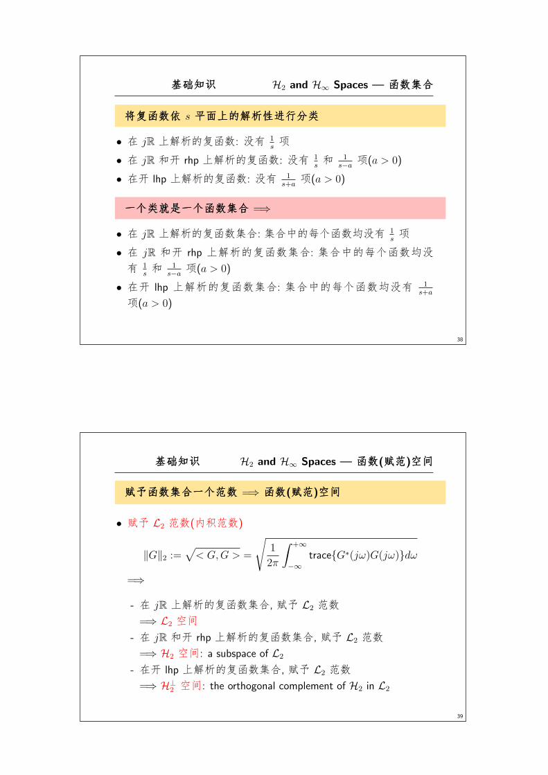
��������� H2 and H∞ Spaces
37
���������������������: ������������������; ���������������(������� ������)
Let f(s) be a complex-valued function defined on S ⊂ C
f(s) is said to be analytic at a point z0 in S if it is differentiable
at z0 and also at each point in some neighborhood of z0
Examples
• G(s) = 1s+1
is analytic on jR and in the open right-half plane
• G(s) = 1sis not analytic on jR
• G(s) = 1s−1
is analytic in the open left-half plane
• ���� G(s) � �����
��: s = σ+ jω ���, s�, jω ��(����), σ > 0 ��
��(���), σ < 0 ����(��)
��������� H2 and H∞ Spaces — ���������
38
������������ s ���������������������������������
• � jR �������: �� 1s�
• � jR �� rhp �������: �� 1s� 1
s−a�(a > 0)
• �� lhp �������: �� 1s+a�(a > 0)
������������ ������������ =⇒
• � jR ��������: ��������� 1s�
• � jR �� rhp ��������: ��������
� 1s� 1
s−a�(a > 0)
• �� lhp ��������: ��������� 1s+a
�(a > 0)
��������� H2 and H∞ Spaces — ������(������)������
39
������������������ ��������� =⇒ ������(������)������
• �� L2 ��(����)
‖G‖2 :=√
< G,G > =
√1
2π
∫ +∞
−∞trace{G∗(jω)G(jω)}dω
=⇒
- � jR ���������, �� L2 ��
=⇒ L2 ��
- � jR �� rhp ���������, �� L2 ��
=⇒ H2 ��: a subspace of L2
- �� lhp ���������, �� L2 ��
=⇒ H⊥2 ��: the orthogonal complement of H2 in L2
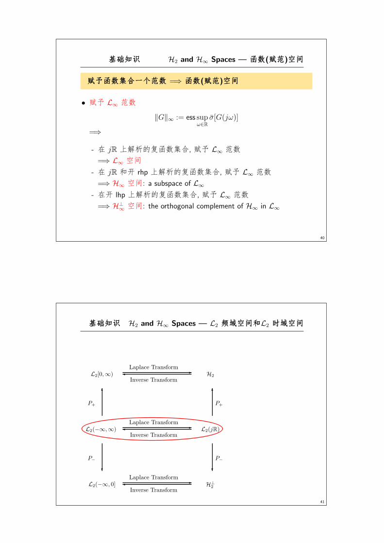
��������� H2 and H∞ Spaces — ������(������)������
40
������������������ ��������� =⇒ ������(������)������
• �� L∞ ��
‖G‖∞ := ess supω∈R
σ[G(jω)]
=⇒
- � jR ���������, �� L∞ ��
=⇒ L∞ ��
- � jR �� rhp ���������, �� L∞ ��
=⇒ H∞ ��: a subspace of L∞- �� lhp ���������, �� L∞ ��
=⇒ H⊥∞ ��: the orthogonal complement of H∞ in L∞
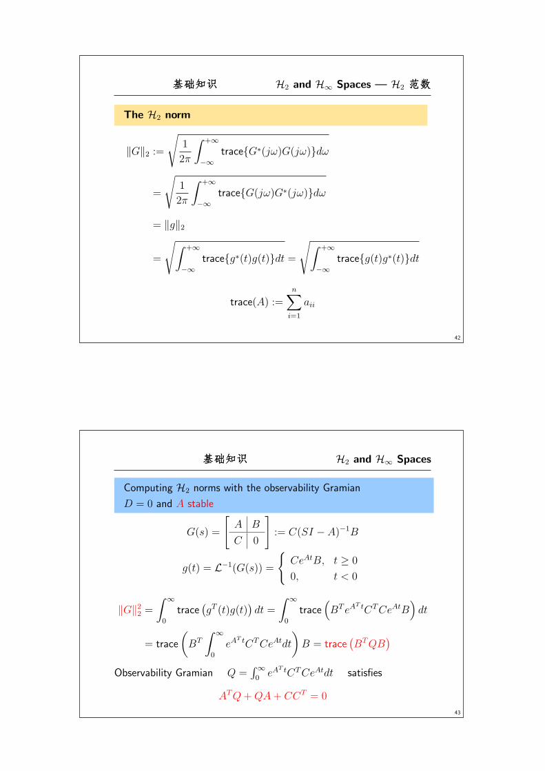
��������� H2 and H∞ Spaces — L2 ���������L2 ������
41
H2
L2(jR)
H⊥2L2(−∞, 0]
L2(−∞,∞)
L2[0,∞)
P−
P+
Laplace Transform
Inverse Transform
Inverse Transform
Laplace Transform
Inverse Transform
Laplace Transform
P−
P+
� �
��
� �
� �
� �
��������� H2 and H∞ Spaces — H2 ������
42
The H2 norm
‖G‖2 :=√
1
2π
∫ +∞
−∞trace{G∗(jω)G(jω)}dω
=
√1
2π
∫ +∞
−∞trace{G(jω)G∗(jω)}dω
= ‖g‖2
=
√∫ +∞
−∞trace{g∗(t)g(t)}dt =
√∫ +∞
−∞trace{g(t)g∗(t)}dt
trace(A) :=n∑
i=1
aii
��������� H2 and H∞ Spaces
43
Computing H2 norms with the observability Gramian
D = 0 and A stable
G(s) =
[A B
C 0
]:= C(SI − A)−1B
g(t) = L−1(G(s)) =
{CeAtB, t ≥ 0
0, t < 0
‖G‖22 =∫ ∞
0
trace(gT (t)g(t)
)dt =
∫ ∞
0
trace(BT eA
T tCTCeAtB)dt
= trace
(BT
∫ ∞
0
eAT tCTCeAtdt
)B = trace
(BTQB
)Observability Gramian Q =
∫∞0
eAT tCTCeAtdt satisfies
ATQ+QA+ CCT = 0
��������� H2 and H∞ Spaces
44
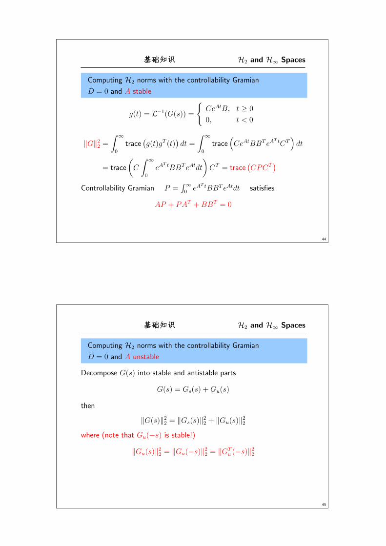
Computing H2 norms with the controllability Gramian
D = 0 and A stable
g(t) = L−1(G(s)) =
{CeAtB, t ≥ 0
0, t < 0
‖G‖22 =∫ ∞
0
trace(g(t)gT (t)
)dt =
∫ ∞
0
trace(CeAtBBT eA
T tCT)dt
= trace
(C
∫ ∞
0
eAT tBBT eAtdt
)CT = trace
(CPCT
)Controllability Gramian P =
∫∞0
eAT tBBT eAtdt satisfies
AP + PAT +BBT = 0
��������� H2 and H∞ Spaces
45
Computing H2 norms with the controllability Gramian
D = 0 and A unstable
Decompose G(s) into stable and antistable parts
G(s) = Gs(s) +Gu(s)
then
‖G(s)‖22 = ‖Gs(s)‖22 + ‖Gu(s)‖22where (note that Gu(−s) is stable!)
‖Gu(s)‖22 = ‖Gu(−s)‖22 = ‖GTu (−s)‖22
��������� H2 and H∞ Spaces
46
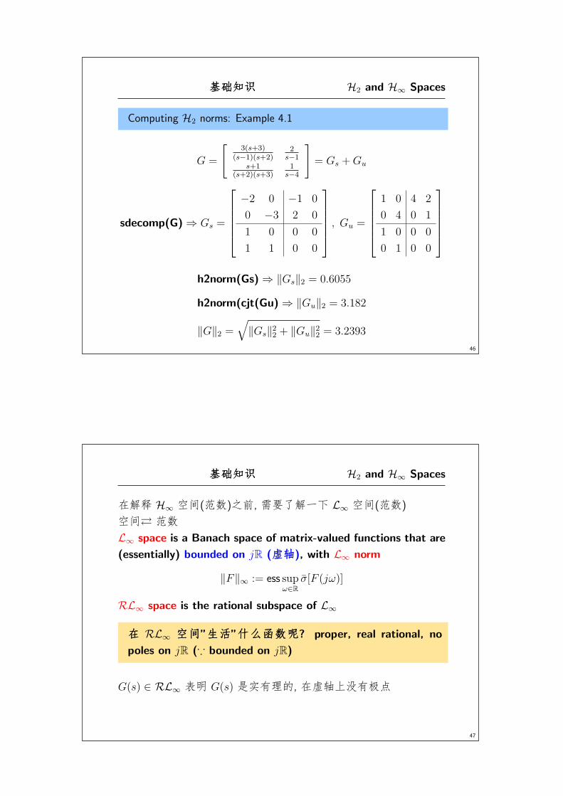
Computing H2 norms: Example 4.1
G =
[3(s+3)
(s−1)(s+2)2
s−1s+1
(s+2)(s+3)1
s−4
]= Gs +Gu
sdecomp(G) ⇒ Gs =
⎡⎢⎢⎢⎢⎣
−2 0 −1 0
0 −3 2 0
1 0 0 0
1 1 0 0
⎤⎥⎥⎥⎥⎦ , Gu =
⎡⎢⎢⎢⎢⎣
1 0 4 2
0 4 0 1
1 0 0 0
0 1 0 0
⎤⎥⎥⎥⎥⎦
h2norm(Gs) ⇒ ‖Gs‖2 = 0.6055
h2norm(cjt(Gu) ⇒ ‖Gu‖2 = 3.182
‖G‖2 =√
‖Gs‖22 + ‖Gu‖22 = 3.2393
��������� H2 and H∞ Spaces
47
��� H∞ ��(��)��, ��� � L∞ ��(��)
��� ��L∞ space is a Banach space of matrix-valued functions that are
(essentially) bounded on jR (������), with L∞ norm
‖F‖∞ := ess supω∈R
σ[F (jω)]
RL∞ space is the rational subspace of L∞
��� RL∞ ������”������”���������������? proper, real rational, no
poles on jR (∵ bounded on jR)
G(s) ∈ RL∞ �� G(s) �����, �������
������ H2 and H∞ Spaces
48
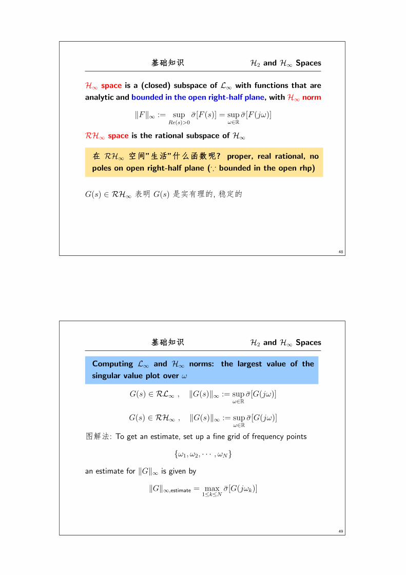
H∞ space is a (closed) subspace of L∞ with functions that are
analytic and bounded in the open right-half plane, with H∞ norm
‖F‖∞ := supRe(s)>0
σ[F (s)] = supω∈R
σ[F (jω)]
RH∞ space is the rational subspace of H∞
��� RH∞ ������”���”���������������? proper, real rational, no
poles on open right-half plane (∵ bounded in the open rhp)
G(s) ∈ RH∞ �� G(s) �����, ���
������ H2 and H∞ Spaces
49
Computing L∞ and H∞ norms: the largest value of the
singular value plot over ω
G(s) ∈ RL∞ , ‖G(s)‖∞ := supω∈R
σ[G(jω)]
G(s) ∈ RH∞ , ‖G(s)‖∞ := supω∈R
σ[G(jω)]
��: To get an estimate, set up a fine grid of frequency points
{ω1, ω2, · · · , ωN}an estimate for ‖G‖∞ is given by
‖G‖∞,estimate = max1≤k≤N
σ[G(jωk)]
������ H2 and H∞ Spaces
50
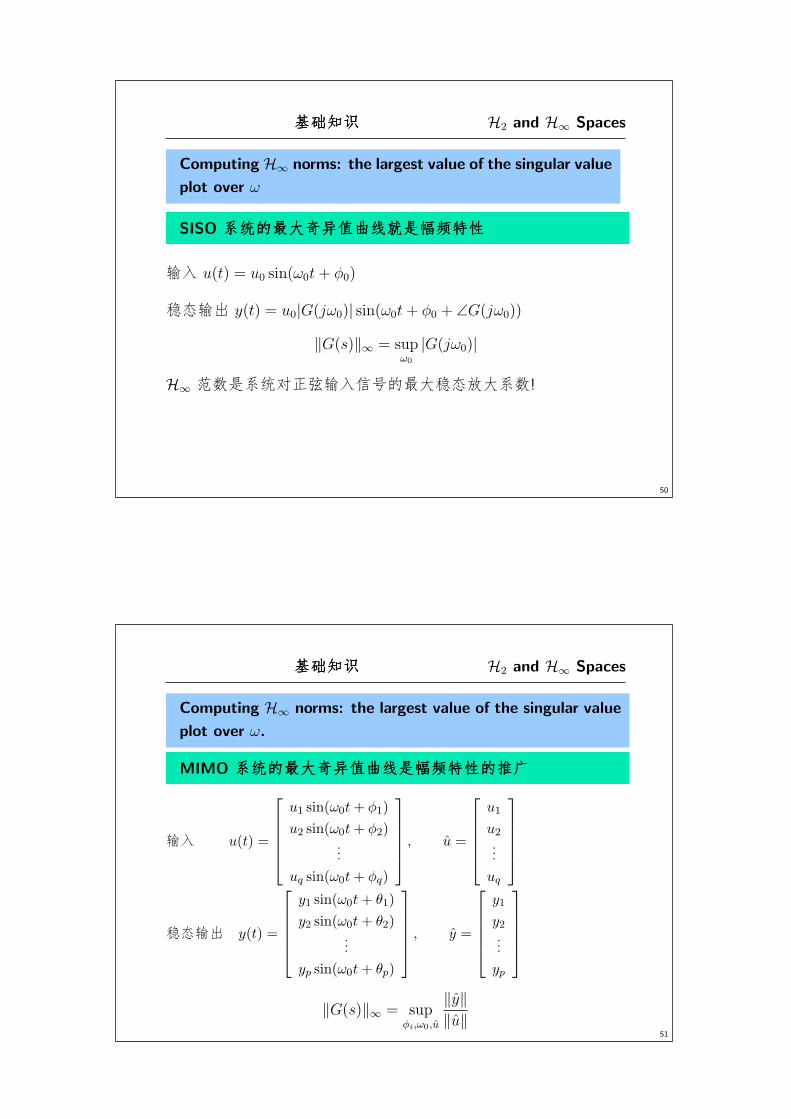
Computing H∞ norms: the largest value of the singular value
plot over ω
SISO ������������������������������������������������
�� u(t) = u0 sin(ω0t+ φ0)
��� y(t) = u0|G(jω0)| sin(ω0t+ φ0 + ∠G(jω0))
‖G(s)‖∞ = supω0
|G(jω0)|
H∞ ���������������������!
��������� H2 and H∞ Spaces
51
Computing H∞ norms: the largest value of the singular value
plot over ω.
MIMO ���������������������������������������������������
�� u(t) =
⎡⎢⎢⎢⎢⎣
u1 sin(ω0t+ φ1)
u2 sin(ω0t+ φ2)...
uq sin(ω0t+ φq)
⎤⎥⎥⎥⎥⎦ , u =
⎡⎢⎢⎢⎢⎣
u1
u2...
uq
⎤⎥⎥⎥⎥⎦
���� y(t) =
⎡⎢⎢⎢⎢⎣
y1 sin(ω0t+ θ1)
y2 sin(ω0t+ θ2)...
yp sin(ω0t+ θp)
⎤⎥⎥⎥⎥⎦ , y =
⎡⎢⎢⎢⎢⎣
y1
y2...
yp
⎤⎥⎥⎥⎥⎦
‖G(s)‖∞ = supφi,ω0,u
‖y‖‖u‖
��������� H2 and H∞ Spaces
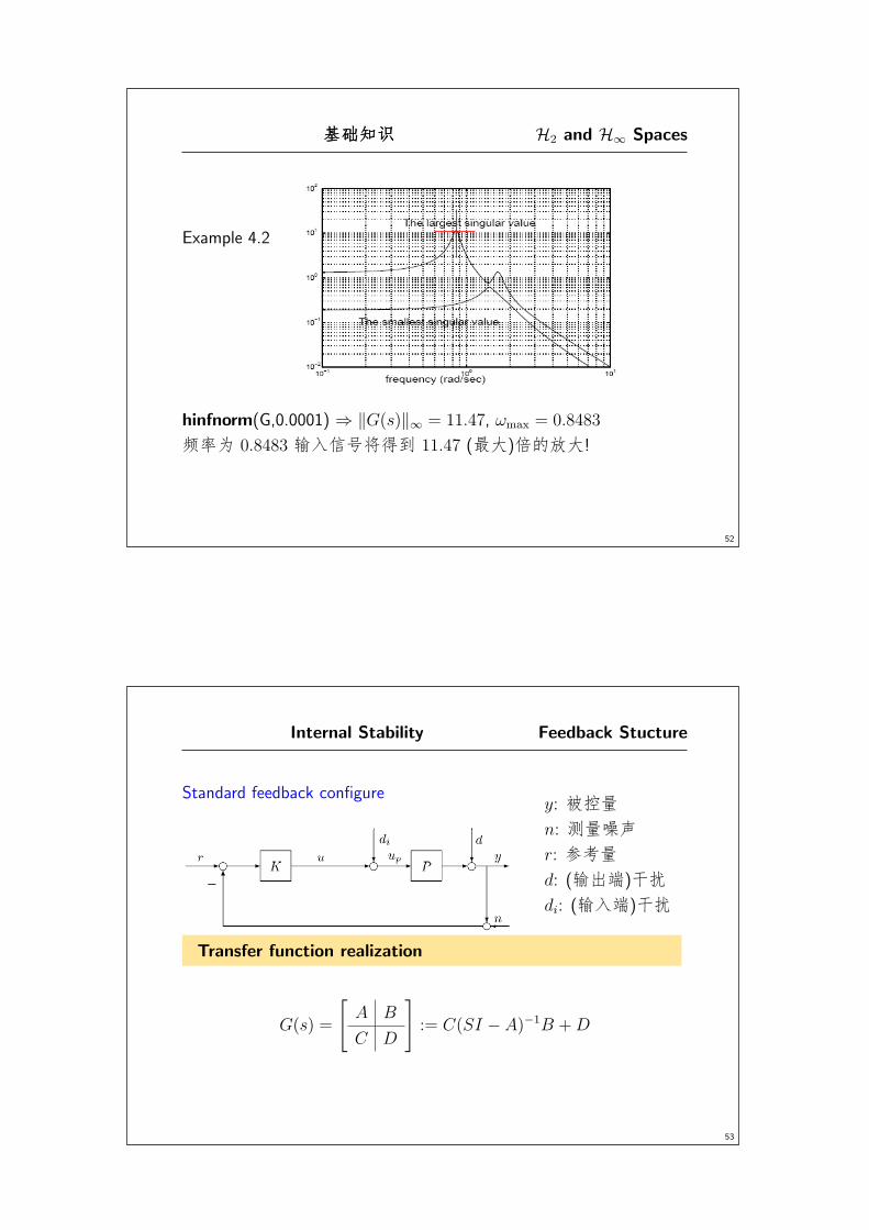
52
Example 4.2
hinfnorm(G,0.0001) ⇒ ‖G(s)‖∞ = 11.47, ωmax = 0.8483
��� 0.8483 ������� 11.47 (��)����!
Internal Stability Feedback Stucture
53
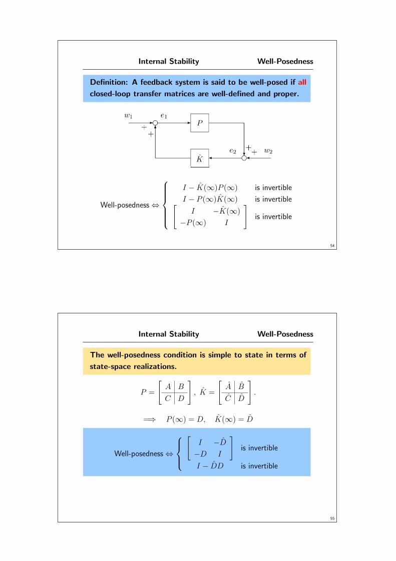
Standard feedback configurey: ���
n: ����
r: ���
d: (���)��
di: (���)��
Transfer function realization
G(s) =
[A B
C D
]:= C(SI − A)−1B +D
Internal Stability Well-Posedness
54
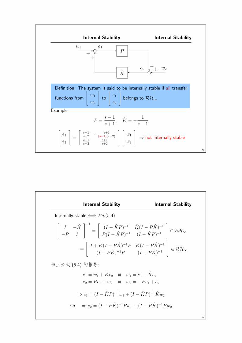
Definition: A feedback system is said to be well-posed if all
closed-loop transfer matrices are well-defined and proper.
Well-posedness ⇔
⎧⎪⎪⎪⎪⎨⎪⎪⎪⎪⎩
I − K(∞)P (∞) is invertible
I − P (∞)K(∞) is invertible[I −K(∞)
−P (∞) I
]is invertible
Internal Stability Well-Posedness
55
The well-posedness condition is simple to state in terms of
state-space realizations.
P =
[A B
C D
], K =
[A B
C D
].
=⇒ P (∞) = D, K(∞) = D
Well-posedness ⇔
⎧⎪⎨⎪⎩[
I −D
−D I
]is invertible
I − DD is invertible
Internal Stability Internal Stability
56
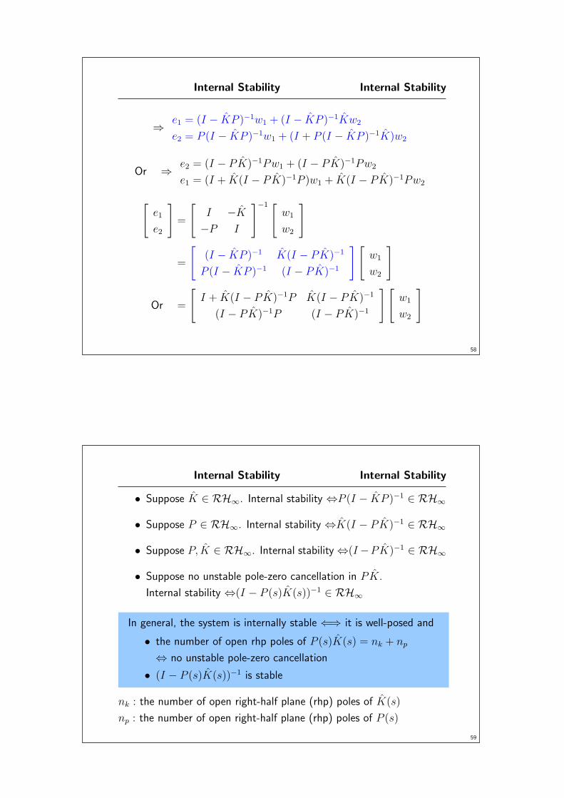
Definition: The system is said to be internally stable if all transfer
functions from
[w1
w2
]to
[e1
e2
]belongs to RH∞
Example
P =s− 1
s+ 1, K = − 1
s− 1[e1
e2
]=
[s+1s+2
− s+1(s−1)(s+2)
s−1s+2
s+1s+2
][w1
w2
]⇒ not internally stable
Internal Stability Internal Stability
57
Internally stable ⇐⇒ Eq.(5.4)[I −K
−P I
]−1
=
[(I − KP )−1 K(I − PK)−1
P (I − KP )−1 (I − KP )−1
]∈ RH∞
=
[I + K(I − PK)−1P K(I − PK)−1
(I − PK)−1P (I − PK)−1
]∈ RH∞
���� (5.4) ����
e1 = w1 + Ke2 ⇔ w1 = e1 − Ke2
e2 = Pe1 + w2 ⇔ w2 = −Pe1 + e2
⇒ e1 = (I − KP )−1w1 + (I − KP )−1Kw2
Or ⇒ e2 = (I − PK)−1Pw1 + (I − PK)−1Pw2
Internal Stability Internal Stability
58
⇒ e1 = (I − KP )−1w1 + (I − KP )−1Kw2
e2 = P (I − KP )−1w1 + (I + P (I − KP )−1K)w2
Or ⇒ e2 = (I − PK)−1Pw1 + (I − PK)−1Pw2
e1 = (I + K(I − PK)−1P )w1 + K(I − PK)−1Pw2
[e1
e2
]=
[I −K
−P I
]−1 [w1
w2
]
=
[(I − KP )−1 K(I − PK)−1
P (I − KP )−1 (I − PK)−1
][w1
w2
]
Or =
[I + K(I − PK)−1P K(I − PK)−1
(I − PK)−1P (I − PK)−1
][w1
w2
]
Internal Stability Internal Stability
59
• Suppose K ∈ RH∞. Internal stability ⇔P (I − KP )−1 ∈ RH∞
• Suppose P ∈ RH∞. Internal stability ⇔K(I − PK)−1 ∈ RH∞
• Suppose P, K ∈ RH∞. Internal stability ⇔(I−PK)−1 ∈ RH∞
• Suppose no unstable pole-zero cancellation in PK.
Internal stability ⇔(I − P (s)K(s))−1 ∈ RH∞
In general, the system is internally stable ⇐⇒ it is well-posed and
• the number of open rhp poles of P (s)K(s) = nk + np
⇔ no unstable pole-zero cancellation
• (I − P (s)K(s))−1 is stable
nk : the number of open right-half plane (rhp) poles of K(s)
np : the number of open right-half plane (rhp) poles of P (s)
Internal Stability Internal Stability
60
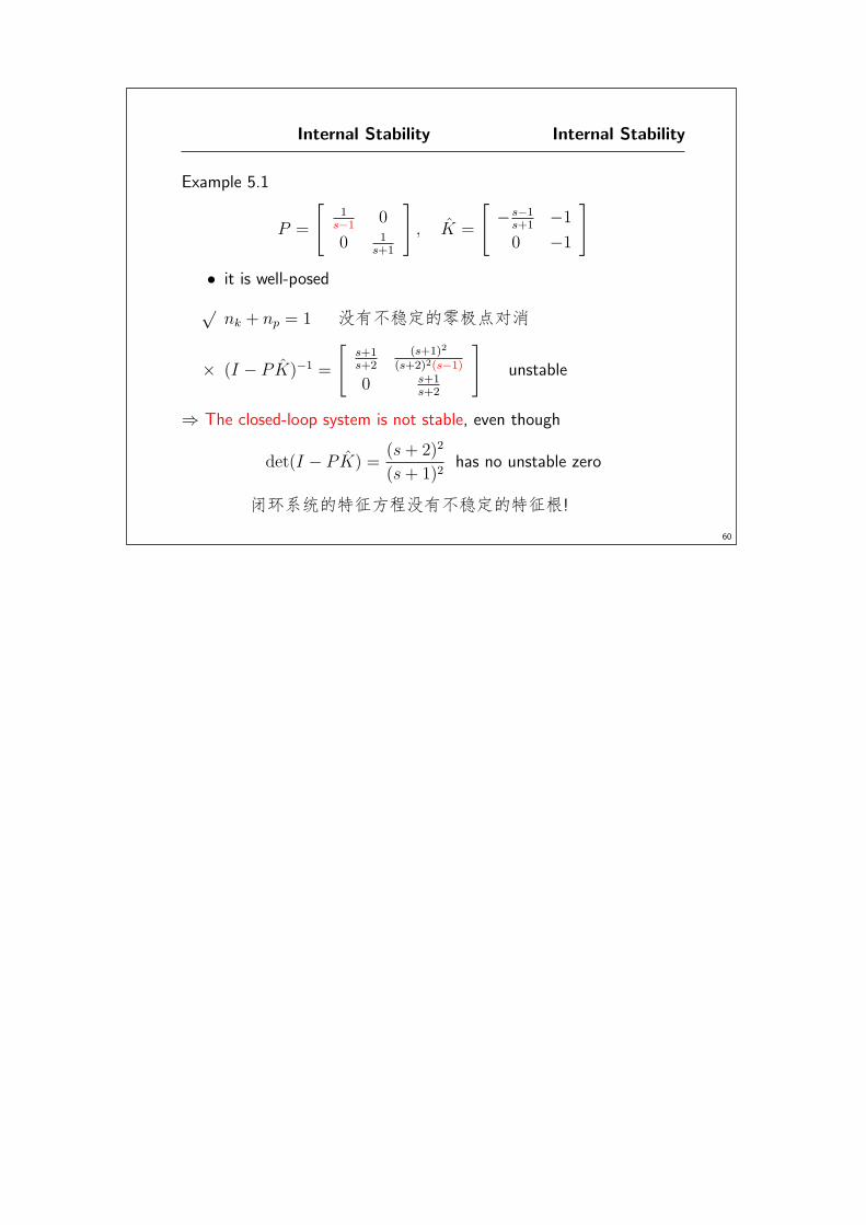
Example 5.1
P =
[1
s−10
0 1s+1
], K =
[− s−1
s+1−1
0 −1
]
• it is well-posed
√nk + np = 1 ����������
× (I − PK)−1 =
[s+1s+2
(s+1)2
(s+2)2(s−1)
0 s+1s+2
]unstable
⇒ The closed-loop system is not stable, even though
det(I − PK) =(s+ 2)2
(s+ 1)2has no unstable zero
���������������!