Lecture 24 - YU

Phys. 441: Nuclear Physics 1Physics Department

Yarmouk University 21163 Irbid Jordan

Chapter 8 :γ Decay

Lecture 24

http://ctaps.yu.edu.jo/physics/Courses/Phys441/Lec8-1

© Dr. Nidal Ershaidat

� ��

٢IntroductionThe gamma decay is the emission of an energetic photon when an excited state of a nucleus decays to a lower energy state. In general a series of γγγγ decays is necessary to reach the stable ground state.These decays are encountered each time a nucleus is excited. This excitation could be the result of α or βdecays or a nuclear reaction.

* λ(F) = E/hc = E(Mev)/1240

The resulting photons are just like the atomic X-rays in nature,i.e. they are electromagnetic radiations, but are more energetic (roughly 0.1 to 10 MeV, wavelengths are between 104 F and 100 F*)

� ��

٣Importance of γ spectroscopy

γ photons are relatively easy to detect which makes them a very popular tool for spectroscopists.

The study of the competitive process to gamma decay namely, the internal conversion, is an excellent tool to obtain the spins and parities of nuclear states!

The Study of excited states is very rich in information about the nuclei properties (See chapter 3).

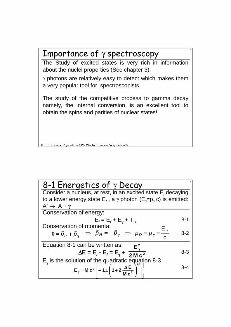
٤8-1 Energetics of γ DecayConsider a nucleus, at rest, in an excited state Ei decaying to a lower energy state Ef , a γ photon (Eγ=pγ c) is emitted: A* → A + γ

8-2γγγγ++++==== ppR

rr0

Eγ is the solution of the quadratic equation 8-38-4

∆∆∆∆++++±±±±−−−−====γγγγ

21

22

cME

211cME

Equation 8-1 can be written as:∆∆∆∆E = Ei - Ef = Eγγγγ + 8-32

2

cM2

E γγγγ

Conservation of momenta:

c

E γγ ==⇒ ppRγ−=⇒ ppR

rr

Conservation of energy:Ei = Ef + Eγ + TR 8-1

� ��

٥

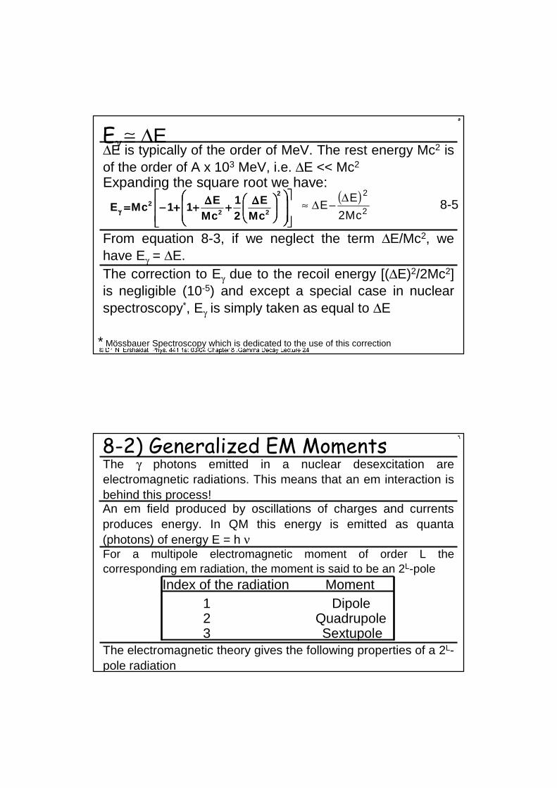
Eγ ≅ ∆E∆E is typically of the order of MeV. The rest energy Mc2 is of the order of A x 103 MeV, i.e. ∆E << Mc2

Expanding the square root we have:

8-5

∆∆∆∆++++∆∆∆∆++++++++−−−−====γγγγ

2

222

cME

21

cME

11cME

From equation 8-3, if we neglect the term ∆E/Mc2, we have Eγ = ∆E.The correction to Eγ due to the recoil energy [(∆E)2/2Mc2] is negligible (10-5) and except a special case in nuclear spectroscopy*, Eγ is simply taken as equal to ∆E

* Mössbauer Spectroscopy which is dedicated to the use of this correction

( )2

2

cM2

EE

∆−∆≈

٦8-2) Generalized EM Moments

For a multipole electromagnetic moment of order L the corresponding em radiation, the moment is said to be an 2L-pole

The electromagnetic theory gives the following properties of a 2L-pole radiation

Index of the radiation1 Dipole2 Quadrupole3 Sextupole

Moment

The γ photons emitted in a nuclear desexcitation are electromagnetic radiations. This means that an em interaction isbehind this process! An em field produced by oscillations of charges and currents produces energy. In QM this energy is emitted as quanta (photons) of energy E = h ν

� ��

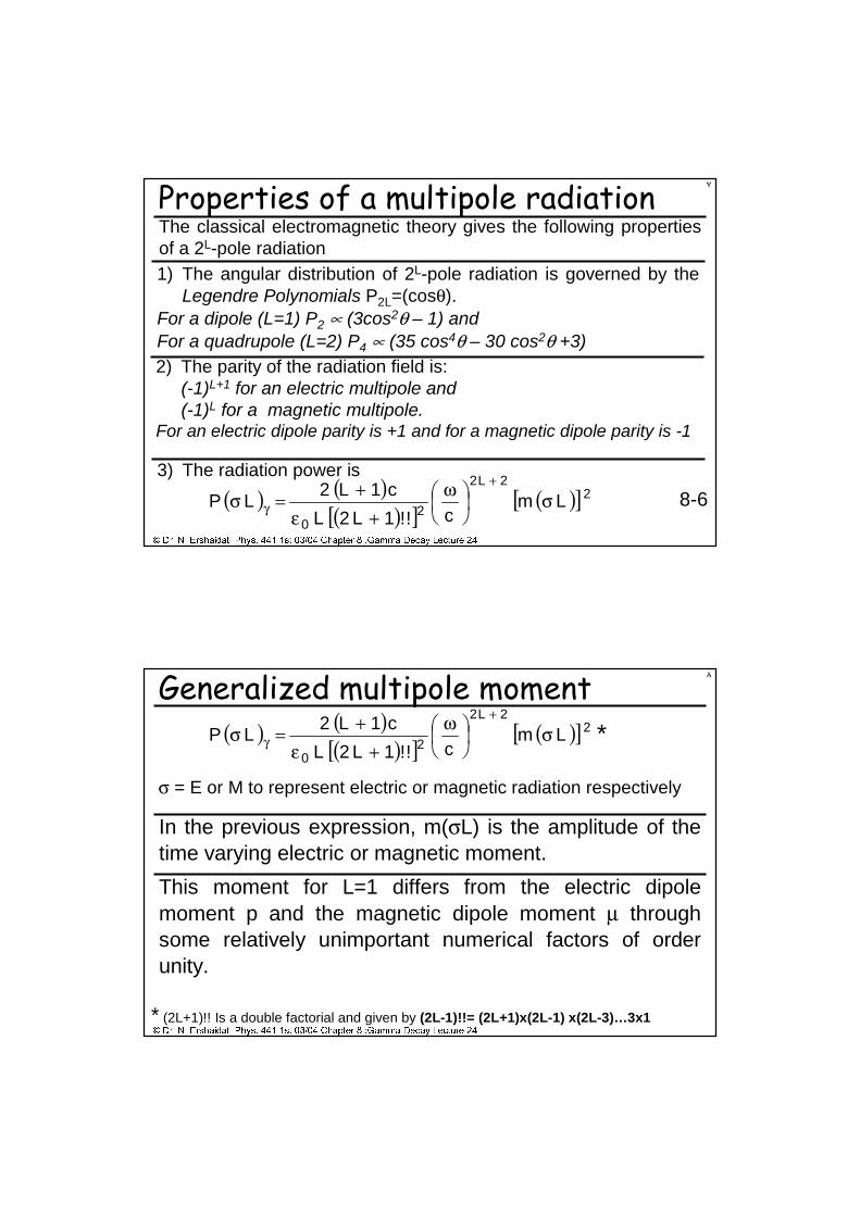
٧Properties of a multipole radiationThe classical electromagnetic theory gives the following properties of a 2L-pole radiation1) The angular distribution of 2L-pole radiation is governed by the

Legendre Polynomials P2L=(cosθ).For a dipole (L=1) P2 ∝ (3cos2θ – 1) andFor a quadrupole (L=2) P4 ∝ (35 cos4θ – 30 cos2θ +3)2) The parity of the radiation field is:

(-1)L+1 for an electric multipole and (-1)L for a magnetic multipole.

For an electric dipole parity is +1 and for a magnetic dipole parity is -1

3) The radiation power is

( ) ( )( )[ ]

( )[ ]22L2

20

Lmc!!1L2L

c1L2LP σ

ω

+ε+=σ

+

γ 8-6

� ��

٨Generalized multipole moment

In the previous expression, m(σL) is the amplitude of the time varying electric or magnetic moment.

This moment for L=1 differs from the electric dipole moment p and the magnetic dipole moment µ through some relatively unimportant numerical factors of order unity.

( ) ( )( )[ ]

( )[ ]22L2

20

Lmc!!1L2L

c1L2LP σ

ω

+ε+=σ

+

γ *

* (2L+1)!! Is a double factorial and given by (2L-1)!!= (2L+1)x(2L-1) x(2L-3)…3x1

σ = E or M to represent electric or magnetic radiation respectively

� ��

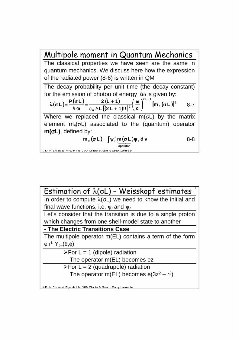
٩Multipole moment in Quantum Mechanics

Where we replaced the classical m(σL) by the matrix element mfi(σL) associated to the (quantum) operator m(σσσσL), defined by:

The classical properties we have seen are the same in quantum mechanics. We discuss here how the expression of the radiated power (8-6) is written in QM

(((( )))) (((( )))) (((( ))))(((( ))))[[[[ ]]]] (((( ))))[[[[ ]]]]2

1L2

20

Lmc!!1L2L

1L2LPL σσσσ

ωωωω

++++εεεε++++====

ωωωωσσσσ====σσσσλλλλ

++++

fihh

The decay probability per unit time (the decay constant) for the emission of photon of energy ω is given by:h

(((( )))) (((( )))) vdLmLmoperator

*∫∫∫∫ ψψψψσσσσψψψψ====σσσσ iffi 321 8-8

8-7

� ��

١٠Estimation of λ(σL) – Weisskopf estimates

- The Electric Transitions Case

In order to compute λ(σL) we need to know the initial and final wave functions, i.e. ψi and ψf

Let’s consider that the transition is due to a single proton which changes from one shell-model state to another

For L = 1 (dipole) radiationThe operator m(EL) becomes ez

The multipole operator m(EL) contains a term of the form e rL Ylm(θ,φ)

For L = 2 (quadrupole) radiationThe operator m(EL) becomes e(3z2 – r2)

� ��

١١

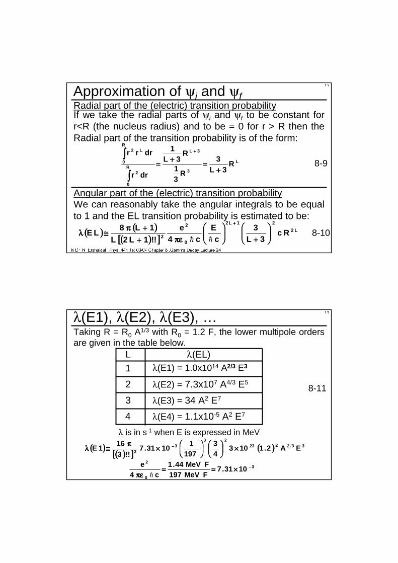
Approximation of ψi and ψfRadial part of the (electric) transition probabilityIf we take the radial parts of ψi and ψf to be constant for r<R (the nucleus radius) and to be = 0 for r > R then the Radial part of the transition probability is of the form:

L

3

3L

R

0

2

R

0

L2

R3L

3

R31

R3L

1

drr

drrr

++++====++++====

++++

∫∫∫∫

∫∫∫∫8-9

Angular part of the (electric) transition probabilityWe can reasonably take the angular integrals to be equal to 1 and the EL transition probability is estimated to be:

(((( )))) (((( ))))(((( ))))[[[[ ]]]]

L2

21L2

0

2

2 Rc3L

3c

Ec4

e!!1L2L1L8

LE

++++

πεπεπεπε++++

++++ππππ≅≅≅≅λλλλ++++

hh8-10

١٢λ(E1), λ(E2), λ(E3), …Taking R = R0 A1/3 with R0 = 1.2 F, the lower multipole orders are given in the table below.

3

0

2

1031.7FMeV197FMeV44.1

c4e −−−−××××========

πεπεπεπε h

(((( )))) (((( ))))[[[[ ]]]] (((( )))) 33222323

32 EA2.1103

43

1971

1031.7!!3

161E ××××

××××

ππππ≅≅≅≅λλλλ −−−−

L λ(EL)1 λ(E1) = 1.0x1014 A2/3 E3

2 λ(E2) = 7.3x107 A4/3 E5

3 λ(E3) = 34 A2 E7

4 λ(E4) = 1.1x10-5 A2 E7

λ is in s-1 when E is expressed in MeV

8-11

� ��

١٣

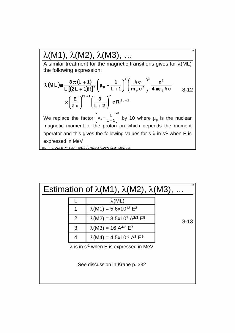
λ(M1), λ(M2), λ(M3), …A similar treatment for the magnetic transitions gives for λ(ML) the following expression:

(((( )))) (((( ))))(((( ))))[[[[ ]]]]

2L2

21L2

0

22

2p

2

p2

Rc2L

3c

E

c4e

cmc

1L1

!!1L2L1L8

LM

−−−−++++

++++

××××

πεπεπεπε

++++

−−−−µµµµ++++

++++ππππ≅≅≅≅λλλλ

h

h

h

8-12

We replace the factor by 10 where µp is the nuclear

magnetic moment of the proton on which depends the moment

operator and this gives the following values for s λ in s-1 when E is

expressed in MeV

2

p 1L1

++++

−−−−µµµµ

١٤

Estimation of λ(M1), λ(M2), λ(M3), …L λ(ML)

1 λ(M1) = 5.6x1013 E3

2 λ(M2) = 3.5x107 A2/3 E5

3 λ(M3) = 16 A4/3 E7

4 λ(M4) = 4.5x10-6 A2 E9

See discussion in Krane p. 332

8-13

λ is in s-1 when E is expressed in MeV

� ��

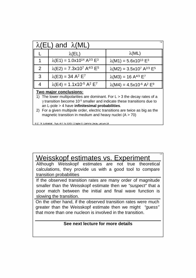
١٥λ(EL) and λ(ML)L λ(EL)1 λ(E1) = 1.0x1014 A2/3 E3

2 λ(E2) = 7.3x107 A4/3 E5

3 λ(E3) = 34 A2 E7

4 λ(E4) = 1.1x10-5 A2 E7

λ(ML)

λ(M1) = 5.6x1013 E3

λ(M2) = 3.5x107 A2/3 E5

λ(M3) = 16 A4/3 E7

λ(M4) = 4.5x10-6 A2 E9

Two major conclusions:1) The lower multipolarities are dominant. For L > 3 the decay rates of a

γ transition become 10-5 smaller and indicate these transitions due to an L-pole > 4 have infinitesimal probabilities.

2) For a given multipole order, electric transitions are twice as big as the magnetic transition in medium and heavy nuclei (A > 70)

١٦

Weisskopf estimates vs. ExperimentAlthough Weisskopf estimates are not true theoretical calculations, they provide us with a good tool to compare transition probabilitiesIf the observed transition rates are many order of magnitude smaller than the Weisskopf estimate then we “suspect” that a poor match between the initial and final wave function is slowing the transition. On the other hand, if the observed transition rates were much greater than the Weisskopf estimate then we might “guess”that more than one nucleon is involved in the transition.

See next lecture for more details

Phys. 441: Nuclear Physics 1Physics Department

Yarmouk University 21163 Irbid Jordan8-2 : Lifetimes for γ Emission,8-3 : Selection Rules

Lecture 25

http://ctaps.yu.edu.jo/physics/Courses/Phys441/Lec8-1

© Dr. Nidal Ershaidat

8-2 : Lifetimes for γ Emission

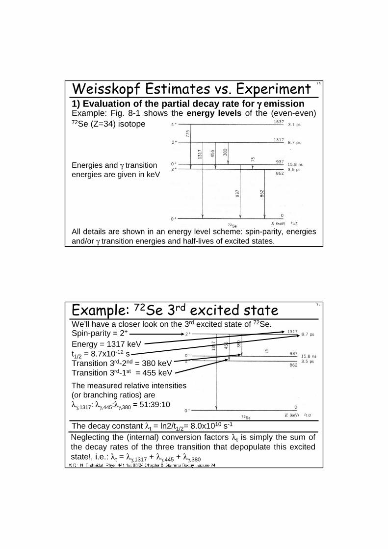
١٩Weisskopf Estimates vs. ExperimentExample: Fig. 8-1 shows the energy levels of the (even-even) 72Se (Z=34) isotope

1) Evaluation of the partial decay rate for γγγγ emission

All details are shown in an energy level scheme: spin-parity, energies and/or γ transition energies and half-lives of excited states.

Energies and γ transition energies are given in keV

� ��

٢٠Example: 72Se 3rd excited stateWe’ll have a closer look on the 3rd excited state of 72Se.Spin-parity = 2+

The decay constant λt = ln2/t1/2= 8.0x1010 s-1

Energy = 1317 keVt1/2 = 8.7x10-12 s

Transition 3rd-1st = 455 keVTransition 3rd-2nd = 380 keV

Neglecting the (internal) conversion factors λt is simply the sum of the decay rates of the three transition that depopulate this excited state!, i.e.: λt = λγ,1317 + λγ,445 + λγ,380

The measured relative intensities(or branching ratios) are λγ,1317: λγ,445:λγ,380 = 51:39:10

� ��

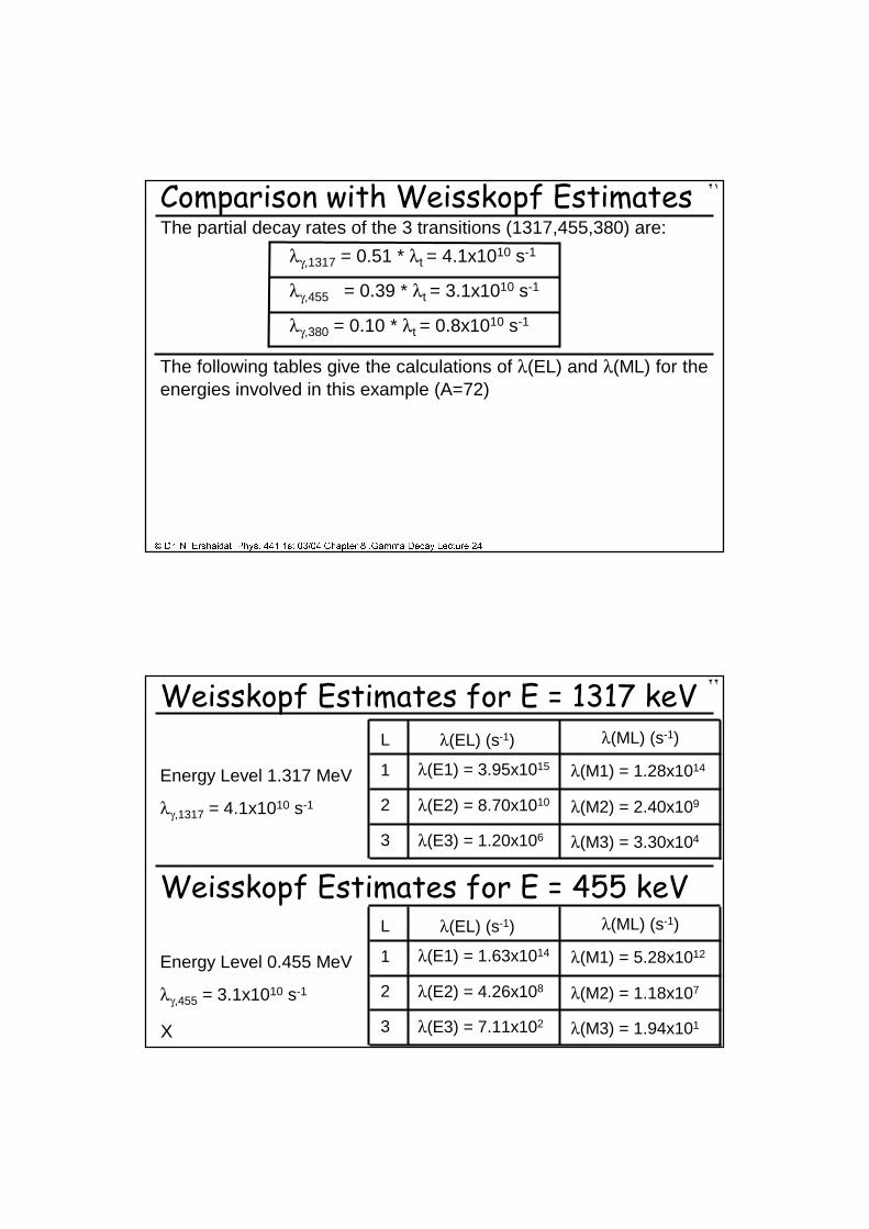
٢١Comparison with Weisskopf Estimates

λγ,1317 = 0.51 * λt = 4.1x1010 s-1

λγ,455 = 0.39 * λt = 3.1x1010 s-1

λγ,380 = 0.10 * λt = 0.8x1010 s-1

The partial decay rates of the 3 transitions (1317,455,380) are:

The following tables give the calculations of λ(EL) and λ(ML) for the energies involved in this example (A=72)

٢٢

λ(EL) (s-1)L

1 λ(E1) = 3.95x1015

2

3 λ(E3) = 1.20x106

λ(ML) (s-1)

λ(M1) = 1.28x1014

λ(M2) = 2.40x109

λ(M3) = 3.30x104

λγ,1317 = 4.1x1010 s-1

Energy Level 1.317 MeV

λ(E2) = 8.70x1010

Weisskopf Estimates for E = 455 keV

Weisskopf Estimates for E = 1317 keV

λ(EL) (s-1)L

1 λ(E1) = 1.63x1014

2

3 λ(E3) = 7.11x102

λ(ML) (s-1)

λ(M1) = 5.28x1012

λ(M2) = 1.18x107

λ(M3) = 1.94x101

λγ,455 = 3.1x1010 s-1


λ(E2) = 4.26x108

X

� ��

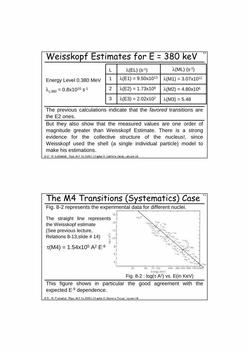
٢٣Weisskopf Estimates for E = 380 keVλ(EL) (s-1)L

1 λ(E1) = 9.50x1013

2

3 λ(E3) = 2.02x102

λ(ML) (s-1)

λ(M1) = 3.07x1012

λ(M2) = 4.80x106

λ(M3) = 5.48

λγ,380 = 0.8x1010 s-1


λ(E2) = 1.73x108

The previous calculations indicate that the favored transitions are the E2 ones. But they also show that the measured values are one order of magnitude greater than Weisskopf Estimate. There is a strong evidence for the collective structure of the nucleus!, since Weisskopf used the shell (a single individual particle) model tomake his estimations.

� ��

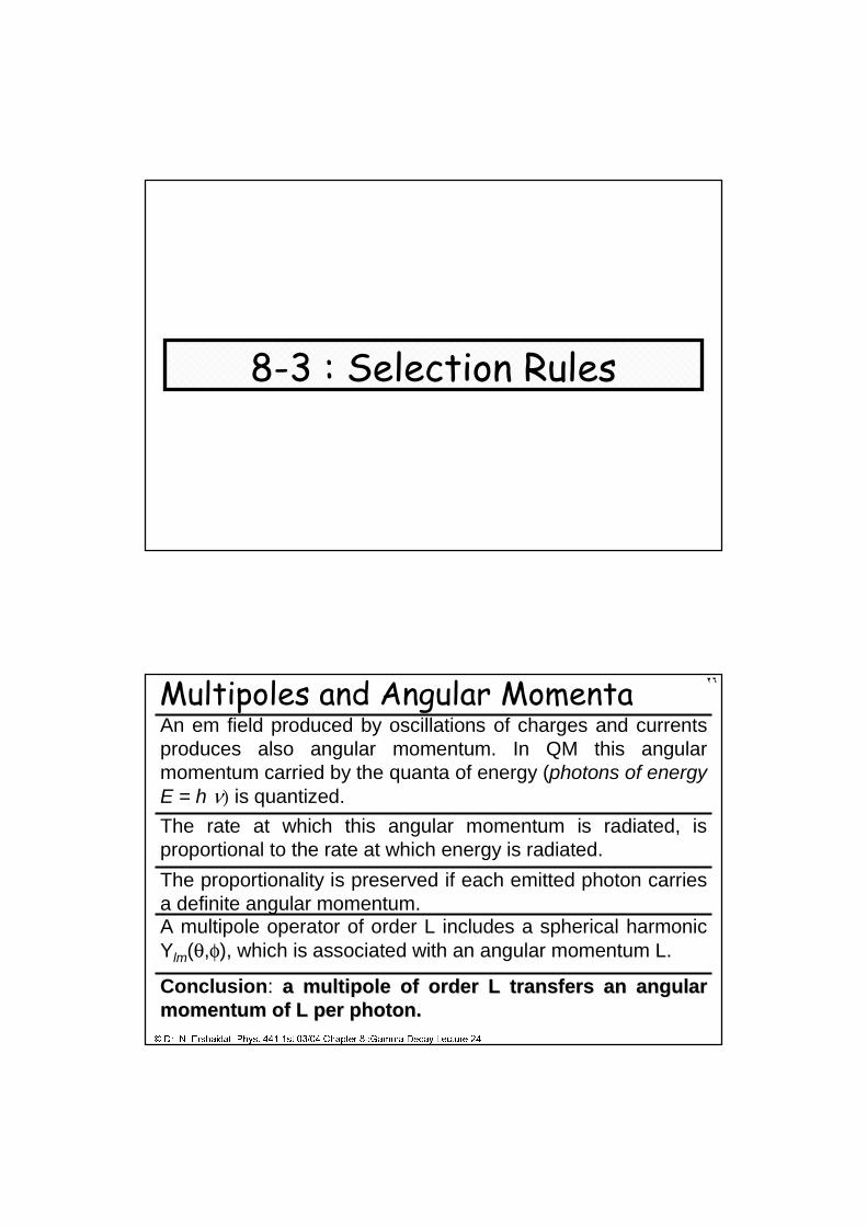
٢٤The M4 Transitions (Systematics) Case

This figure shows in particular the good agreement with the expected E-9 dependence.

Fig. 8-2 represents the experimental data for different nuclei.

The straight line represents the Weisskopf estimate (See previous lecture, Relations 8-13,slide # 14)

τ(M4) = 1.54x105 A2 E-9

Fig. 8-2 : log(τ A2) vs. E(in KeV)

8-3 : Selection Rules

� ��

٢٦Multipoles and Angular MomentaAn em field produced by oscillations of charges and currents produces also angular momentum. In QM this angular momentum carried by the quanta of energy (photons of energy E = h ν) is quantized.

The rate at which this angular momentum is radiated, is proportional to the rate at which energy is radiated.

The proportionality is preserved if each emitted photon carries a definite angular momentum.

Conclusion: a multipole of order L transfers an angular a multipole of order L transfers an angular momentum of L per photon.momentum of L per photon.

A multipole operator of order L includes a spherical harmonic Ylm(θ,φ), which is associated with an angular momentum L.

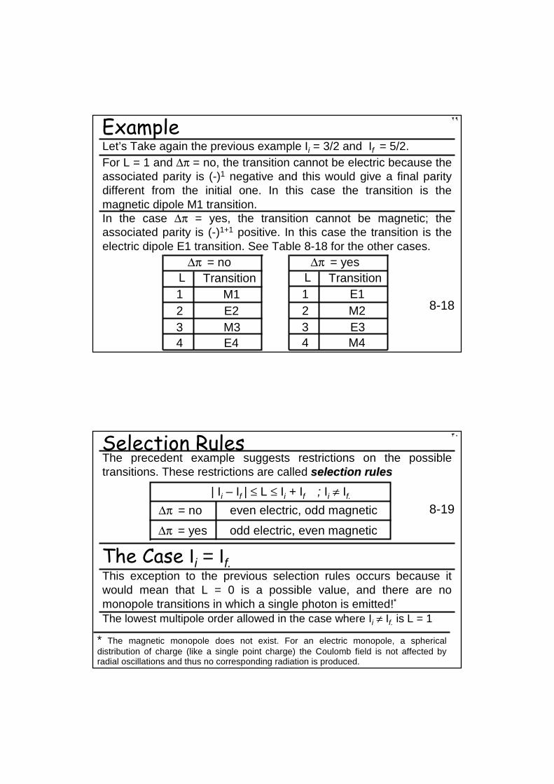
٢٧Angular Momentum and Parity Selection Rules

Example: For Ii = 3/2 and If = 5/2, the possible values for L are:1, 2, 3 and 4 and the radiated field would be a mixture of dipole, quadrupole, octupole and hexadecapole radiation!

Thanks to the rules of addition of angular momenta we know that L could only have restricted values.

8-15| Ii – If | ≤ L ≤ Ii + If

The relative parity of the initial and final levels determine the type of the emitted radiation (electric or magnetic). The following table resumes the parities related to em radiations

Consider a γ transition from an initial excited state of angular momentum Ii and parity πi to a final state (If, πf). Assume Ii ≠ If.(Spin-parity for these states are and respectively)iππππ

iI fππππfI

Conservation of angular momentum is expressed by:LIIrrr

++++==== fi 8-14

٢٨Parity and EM TransitionsThe following table resumes what we know about the parity associated to electric and magnetic transition.

8-16L Electric Transition Magnetic TransitionEven + -Odd - +

Parity

Ii+

If L

+

∆π

∆π = no- -

The following notations are used when studying parity changes –see Table 8-17

++ Even

-- Odd+ ∆π = yes-

- +

8-17

The two tables are used to determine the type of the emitted radiation (electric or magnetic).

٢٩ExampleLet’s Take again the previous example Ii = 3/2 and If = 5/2.

8-18

L Transition∆π = no

2 E23 M3

E44

1 M1L Transition

∆π = yes

2 M23 E3

M44

1 E1

For L = 1 and ∆π = no, the transition cannot be electric because the associated parity is (-)1 negative and this would give a final parity different from the initial one. In this case the transition is the magnetic dipole M1 transition.In the case ∆π = yes, the transition cannot be magnetic; the associated parity is (-)1+1 positive. In this case the transition is the electric dipole E1 transition. See Table 8-18 for the other cases.

٣٠

The Case Ii = If.

Selection RulesThe precedent example suggests restrictions on the possible transitions. These restrictions are called selection rulesselection rules

∆π = no even electric, odd magnetic

| Ii – If | ≤ L ≤ Ii + If ; Ii ≠ If.8-19

∆π = yes odd electric, even magnetic

This exception to the previous selection rules occurs because itwould mean that L = 0 is a possible value, and there are no monopole transitions in which a single photon is emitted!*

* The magnetic monopole does not exist. For an electric monopole, a spherical distribution of charge (like a single point charge) the Coulomb field is not affected by radial oscillations and thus no corresponding radiation is produced.

The lowest multipole order allowed in the case where Ii ≠ If. is L = 1

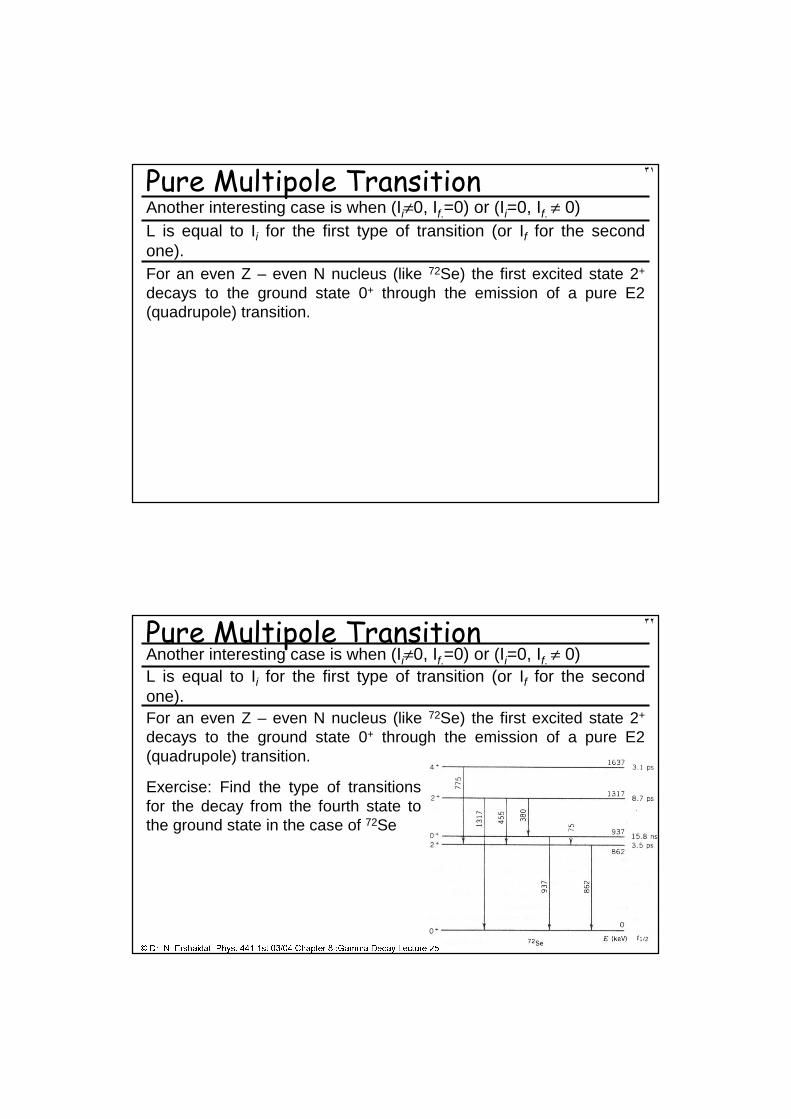
٣١Pure Multipole TransitionAnother interesting case is when (Ii≠0, If.=0) or (Ii=0, If. ≠ 0)L is equal to Ii for the first type of transition (or If for the second one).For an even Z – even N nucleus (like 72Se) the first excited state 2+

decays to the ground state 0+ through the emission of a pure E2 (quadrupole) transition.

� ��

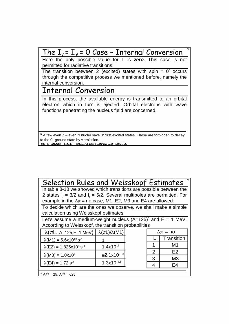
٣٢Pure Multipole TransitionAnother interesting case is when (Ii≠0, If.=0) or (Ii=0, If. ≠ 0)L is equal to Ii for the first type of transition (or If for the second one).For an even Z – even N nucleus (like 72Se) the first excited state 2+

decays to the ground state 0+ through the emission of a pure E2 (quadrupole) transition.

Exercise: Find the type of transitions for the decay from the fourth state to the ground state in the case of 72Se

� ��

٣٣

Internal Conversion

The Ii = If = 0 Case – Internal Conversion

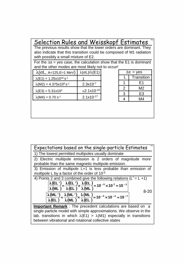
In this process, the available energy is transmitted to an orbital electron which in turn is ejected. Orbital electrons with wave functions penetrating the nucleus field are concerned.

Here the only possible value for L is zero. This case is not permitted for radiative transitions.The transition between 2 (excited) states with spin = 0* occurs through the competitive process we mentioned before, namely the internal conversion.

* A few even Z – even N nuclei have 0+ first excited states. Those are forbidden to decay to the 0+ ground state by γ emission.

٣٤

λ(σL, A=125,E=1 MeV)

λ(E2) = 1.825x109 s-1

λ(M3) = 1.0x104

λ(E4) = 1.72 s-1

λ(σL)/λ(M1)

11.4x10-3

≅2.1x10-10

1.3x10-13

Selection Rules and Weisskopf EstimatesIn table 8-18 we showed which transitions are possible between the 2 states Ii = 3/2 and If = 5/2. Several multipoles are permitted. For example in the ∆π = no case, M1, E2, M3 and E4 are allowed.To decide which are the ones we observe, we shall make a simple calculation using Weisskopf estimates.Let’s assume a medium-weight nucleus (A=125)* and E = 1 MeV. According to Weisskopf, the transition probabilities

λ(M1) = 5.6x1013 s-1 L Transition∆π = no

2 E23 M3

E44

1 M1

* A2/3 = 25, A4/3 = 625

٣٥

λ(σL, A=125,E=1 MeV)

λ(M2) = 4.375x109 s-1

λ(E3) = 5.31x104

λ(M4) = 0.70 s-1

λ(σL)/λ(E1)

12.3x10-7

≅2.1x10-10

2.1x10-17

Selection Rules and Weisskopf EstimatesThe previous results show that the lower orders are dominant. They also indicate that this transition could be composed of M1 radiation with possibly a small mixture of E2.For the ∆π = yes case, the calculation show that the E1 is dominant and the other modes are most likely not to occur!

λ(E1) = 1.25x1016 s-1 L Transition∆π = yes

2 M23 E3

M44

1 E1

٣٦Expectations based on the single-particle Estimates1) The lowest permitted multipoles usually dominate

3) Emission of multipole L+1 is less probable than emission of multipole L by a factor of the order of 10-5

2) Electric multipole emission is 2 orders of magnitude more probable than the same magnetic multipole emission.

4) Points 2 and 3 combined give the following relations (L’ = L +1)(((( ))))(((( ))))

(((( ))))(((( ))))

(((( ))))(((( ))))

325 101010MLEL

EL'EL

ML'EL −−−−−−−− ====××××====

λλλλλλλλ××××

λλλλλλλλ====

λλλλλλλλ

8-20(((( ))))(((( ))))

(((( ))))(((( ))))

(((( ))))(((( ))))

725 101010ELML

ML'ML

EL'ML −−−−−−−−−−−− ====××××====

λλλλλλλλ××××

λλλλλλλλ====

λλλλλλλλ

Important RemarkImportant Remark : The precedent calculations are based on a single particle model with simple approximations. We observe in the lab. transitions in which λ(E1) > λ(M1) especially in transitions between vibrational and rotational collective states

Next Lecture

End of Chapter 8

End of Lecture 25

Lecture 24 - YU

Documents

Transcript of Lecture 24 - YU