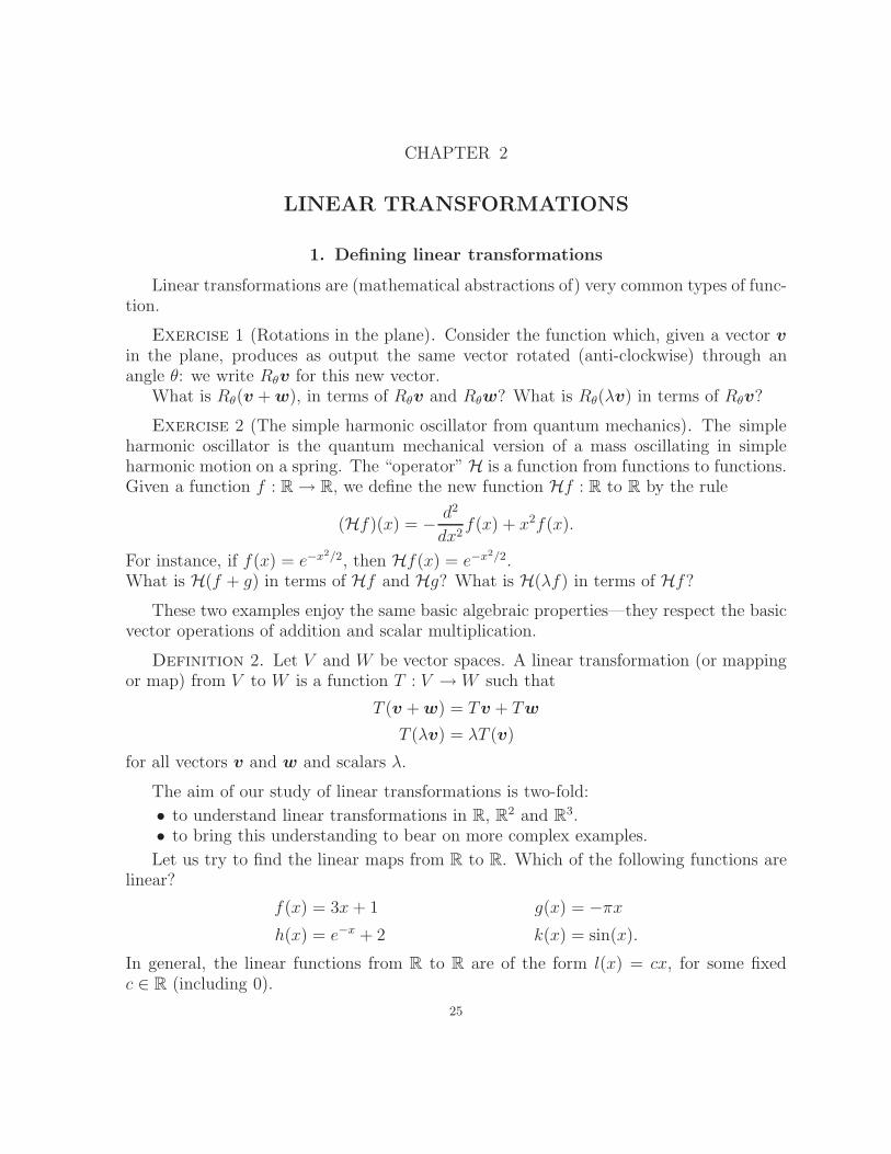
CHAPTER 2

LINEAR TRANSFORMATIONS

1. Defining linear transformations

Linear transformations are (mathematical abstractions of) very common types of func-tion.

Exercise 1 (Rotations in the plane). Consider the function which, given a vector vin the plane, produces as output the same vector rotated (anti-clockwise) through anangle θ: we write Rθv for this new vector.

What is Rθ(v + w), in terms of Rθv and Rθw? What is Rθ(λv) in terms of Rθv?

Exercise 2 (The simple harmonic oscillator from quantum mechanics). The simpleharmonic oscillator is the quantum mechanical version of a mass oscillating in simpleharmonic motion on a spring. The “operator” H is a function from functions to functions.Given a function f : R → R, we define the new function Hf : R to R by the rule

(Hf)(x) = − d2

dx2f(x) + x2f(x).

For instance, if f(x) = e−x2/2, then Hf(x) = e−x2/2.What is H(f + g) in terms of Hf and Hg? What is H(λf) in terms of Hf?

These two examples enjoy the same basic algebraic properties—they respect the basicvector operations of addition and scalar multiplication.

Definition 2. Let V and W be vector spaces. A linear transformation (or mappingor map) from V to W is a function T : V → W such that

T (v + w) = Tv + Tw

T (λv) = λT (v)

for all vectors v and w and scalars λ.

The aim of our study of linear transformations is two-fold:

• to understand linear transformations in R, R2 and R

3.• to bring this understanding to bear on more complex examples.

Let us try to find the linear maps from R to R. Which of the following functions arelinear?

f(x) = 3x + 1 g(x) = −πx

h(x) = e−x + 2 k(x) = sin(x).

In general, the linear functions from R to R are of the form l(x) = cx, for some fixedc ∈ R (including 0).

25

26 2. LINEAR TRANSFORMATIONS

2. Linear Maps and Matrices

Suppose that A is an m × n matrix. Define TA : Rm → R

n by the formula

TAx = Ax for all x ∈ Rm.

Then TA is a linear map. Indeed,

TA(x + y) = A(x + y) = Ax + Ay = TA(x) + TA(y),

and TA(λx) = λTA(x) similarly.In some senses, matrices are the only examples of linear maps.

Theorem 15. Suppose that V and W are vector spaces with bases {v1, . . . , vm} = Aand {w1, . . . , wn} = B respectively, and suppose that T : V → W is a linear map. Let ai

denote the vector Tvi, [ai]B denote its coordinates relative to the basis B, and A denotethe matrix with columns [ai]B. Then for all x in V ,

[Tx]B = A[x]A.

Proof. For x in V ,

x = x1v1 + x2v2 + · · ·+ xmvm,

where (x1, x2, . . . , xm)T = [x]A. Then

Tx = T (x1v1 + x2v2 + · · · + xmvm) = x1Tv1 + x2Tv2 + · · · + xmTvm,

so[Tx]B = x1[Tv1]B + x2[Tv2]B + · · · + xm[Tvm]B = A(x1, x2, . . . , xm)T ,

as required.

Example. Let Rθ : R2 → R

2 be the rotation (anti-clockwise) through the angle θ.Then

Rθ

(10

)=

(cos θsin θ

)

Rθ

(10

)=

(− sin θcos θ

),

in the standard basis for R2. Then

Rθ

(xy

)= xRθ

(10

)+ yRθ

(01

)=

(cos θ − sin θsin θ cos θ

) (xy

).

Example. Let Ds : R3 → R

3 be the dilation by a factor of s in R+. The Dsx = sx

for all x in R3. Thus

Dsx =

s 0 0

0 s 00 0 s

x.

Exercise 3. What is the geometric effect of multiplying by the matrix1 0 0

0 1 00 0 10−3

3. KERNELS AND RANGES 27

in R3?

Exercise 4. What is the geometrical effect of multiplying by the matrix

(1 10 1

)in

R2?

Exercise 5. Let a be a unit vector in R3. Define the map L : R

3 → R3 by the

formula Lx = (x · a)a.

(a) Show that L is linear.(b) Express L as multiplication by a matrix.(c) Describe L geometrically.

Exercise 6. Let a be a unit vector in R3. Define the map X : R

3 → R3 by the

formula

Xv = v × a.

(a) Show that X is linear.(b) Express X as multiplication by a matrix.(c) Describe X geometrically.

3. Kernels and Ranges

Consider the linear system

a11x1 + a12x2 + · · ·+ a1mxn = b1

. . .

am1x1 + am2x2 + · · ·+ amnxn = bm,

or equivalently, in matrix form

Ax = b.

What b can we solve this for? Is the solution unique?We have seen that we can solve the equation if and only if b is a linear combination

of the columns of A; we write b ∈ col(A) for short. We also know that, if xpart is aparticular solution of Ax = b, then every solution is of the form xpart +xhom, where xhom

is a solution of the homogeneous equation

Ax = 0.

If the homogeneous equation has one solution, so does Ax = b; if the homogeneousequation has many solutions, so does Ax = b.

Next, consider the differential equation

Hu(x) = −d2u

dx2(x) + x2u(x) = b(x),

where b is a known function and u is unknown. What b can we solve this for? Is thesolution unique?

We can answer the first question in a formal sense: b must lie in the range of H, alsoknown as the image of H, and written range(H) or image(H). For the second question,

28 2. LINEAR TRANSFORMATIONS

we can show that, if upart is a particular solution of Hu = b, and uhom is any solution ofthe homogeneous equation Hu = 0, then

H(upart + uhom) = b + 0 = b,

i.e., upart + uhom is a solution of Hu = b. In fact, every solution of Hu = b arises in thisway. Thus the uniqueness or nonuniqueness of the solutions of the homogeneous equationcontrols the uniqueness or nonuniqueness of the original equation. We unify these (andother examples) in the following observations.

Let T : V → W be a linear map. The set of vectors TV = {Tv : v ∈ V } is called therange or image of T , and written range(T ) or image(T ). Then range(T ) is the collectionof vectors w in W for which the equation Tx = w can be solved.

Let xpart be a particular solution of the equation Tx = w, and let xhom be any solutionof the homogeneous equation Txhom = 0. Then

T (xpart + xhom) = T (xpart) + T (xhom) = w + 0 = w,

so that xpart +xhom is a solution of Tx = w. Further, every solution of Tx = w is of thisform. Indeed, if Tx = w and Txpart = w, then

T (x − xpart) = T (x) − T (xpart) = w − w = 0,

so x − xpart is a solution of the homogeneous equation.Given a linear map T : V → W , we define the kernel of T , written ker(T ), to be the

subspace of V consisting of all solutions of the homogeneous equation Tx = 0; in symbols

ker(T ) = {x ∈ V : Tx = 0}.

4. Rank and nullity

We define the nullity of T , written nullity(T ), to be the dimension of ker(T ). This isequal to the number of parameters in the solution of Tx = w.

Example. The general solution of

d2

dx2u(x) − u(x) = x

is

u(x) = −x + A sin x + B cos x.

This has two parameters, because the nullity of the differential operator T : Tf(x) =f ′′(x) − f(x), is 2.

Suppose that V and W are vector spaces, and that T : V → W is a linear map.The dimension of T (V ) (also known as image(T ) or range(T )) is called the rank of T .Sometimes the number dim(W ) − dim(T (V )) is called the co-rank of T . Obviously therank determines the co-rank, and vice versa.

Proposition 16. Suppose that T : V → W is a linear map. Then

(i) T is one-to-one if and only if nullity(T ) = 0.(ii) T is onto if and only if rank(T ) = dim(W ), i.e., if and only if co-rank(T ) = 0.

4. RANK AND NULLITY 29

Theorem 17. If U is a subspace of W , then the smallest number of equations neededto describe U is dim(W ) − dim(U).

Example. Consider the line with parametric equation x = λd, where d = (2, 0, 1)T .This line is a one-dimensional subspace. It may also be described by the equations y = 0and x = 2z. It is of codimension 2.

Challenge Problem. Find equations which define span{(1, 2, 0, 1)T , (1, 0, 2, 0)T

}in R

4. What is the minimal number of equations?

We conclude that the co-rank of a linear transformation T : Rm → R

n is the numberof equations needed to describe the image of T .

Theorem 18 (The rank-nullity theorem for matrices). Suppose that A ∈ Mm,n. Then

rank(A) + nullity(A) = m.

Proof. Suppose that A is row-reduced to row-echelon form. Then the columns of Acorresponding to the leading columns of the reduced matrix form a basis for range(A),hence rank(A) is equal to the number of leading columns. The nonleading columns ofthe reduced matrix correspond to the parameters of the solution, i.e., nullity(A) is equalto the number of nonleading columns. These numbers add to give the total number ofcolumns, i.e., m.

Corollary 19. If A is a square matrix, then nullity(A) = co-rank(A). Consequently,the linear transformations associated to square matrices are one-to-one if and only if theyare onto.

Example. Consider D : Pn → Pn−1, given by

D(antn + · · ·+ a0) = nantn−1 + · · ·+ a1

(i.e., D corresponds to differentiation). By choosing the coefficients an, an−1, . . . , a1

correctly, we can arrange that the right hand side is any polynomial of degree n − 1.Thus range(D) = Pn−1, and hence rank(D) = dim(Pn−1) = n. Also, the kernel of Dis the set of all constant polynomials: indeed, D(ant

n + · · · + a0) = 0 if and only ifan = an−1 = · · · = a1 = 0, and the polynomial is constant. Then nullity(D) = 1. Finally,rank(D) + nullity(D) = n + 1 = dim(Pn).

Exercise 7. Find the nullity of the matrix1 2 3 4

1 0 4 21 −1 0 0

.

Answer. Reduce to row-echelon form. The reduced matrix is of the form1 ∗ ∗ ∗

0 ∗ ∗ ∗0 0 ∗ ∗

.

Then the rank of the matrix is 3 and the nullity is 1. �Note that we do not have to find ker(T ) explicitly to show that it is one-dimensional.

30 2. LINEAR TRANSFORMATIONS

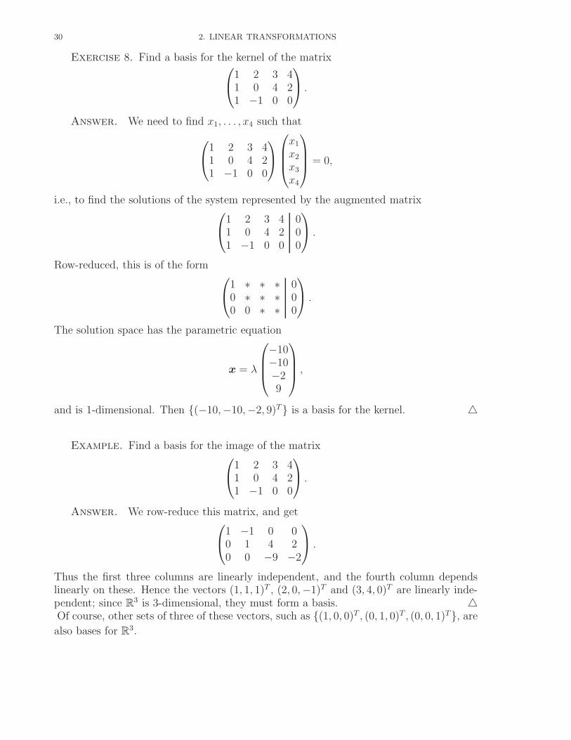
Exercise 8. Find a basis for the kernel of the matrix1 2 3 4

1 0 4 21 −1 0 0

.

Answer. We need to find x1, . . . , x4 such that

1 2 3 4

1 0 4 21 −1 0 0

x1

x2

x3

x4

= 0,

i.e., to find the solutions of the system represented by the augmented matrix1 2 3 4

1 0 4 21 −1 0 0

000

.

Row-reduced, this is of the form 1 ∗ ∗ ∗

0 ∗ ∗ ∗0 0 ∗ ∗

000

.

The solution space has the parametric equation

x = λ

−10−10−29

,

and is 1-dimensional. Then {(−10,−10,−2, 9)T} is a basis for the kernel. �

Example. Find a basis for the image of the matrix1 2 3 4

1 0 4 21 −1 0 0

.

Answer. We row-reduce this matrix, and get1 −1 0 0

0 1 4 20 0 −9 −2

.

Thus the first three columns are linearly independent, and the fourth column dependslinearly on these. Hence the vectors (1, 1, 1)T , (2, 0,−1)T and (3, 4, 0)T are linearly inde-pendent; since R

3 is 3-dimensional, they must form a basis. �Of course, other sets of three of these vectors, such as {(1, 0, 0)T , (0, 1, 0)T , (0, 0, 1)T}, are

also bases for R3.

4. RANK AND NULLITY 31

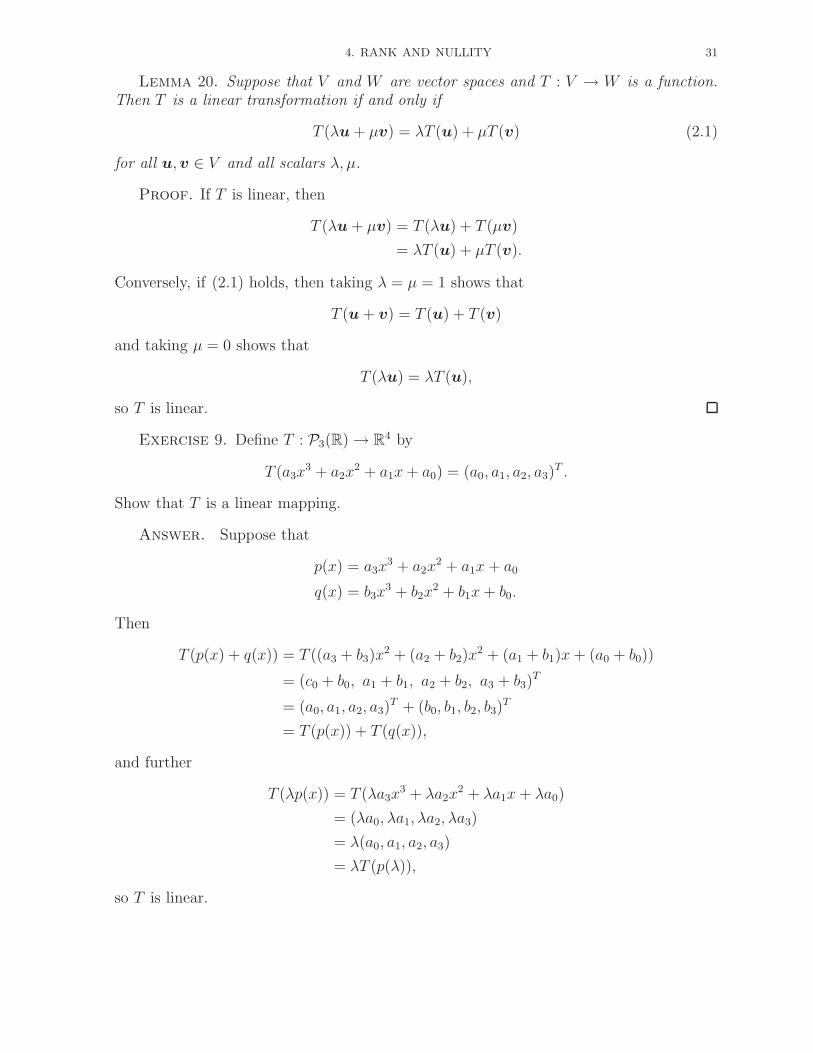
Lemma 20. Suppose that V and W are vector spaces and T : V → W is a function.Then T is a linear transformation if and only if

T (λu + µv) = λT (u) + µT (v) (2.1)

for all u, v ∈ V and all scalars λ, µ.

Proof. If T is linear, then

T (λu + µv) = T (λu) + T (µv)

= λT (u) + µT (v).

Conversely, if (2.1) holds, then taking λ = µ = 1 shows that

T (u + v) = T (u) + T (v)

and taking µ = 0 shows that

T (λu) = λT (u),

so T is linear.

Exercise 9. Define T : P3(R) → R4 by

T (a3x3 + a2x

2 + a1x + a0) = (a0, a1, a2, a3)T .

Show that T is a linear mapping.

Answer. Suppose that

p(x) = a3x3 + a2x

2 + a1x + a0

q(x) = b3x3 + b2x

2 + b1x + b0.

Then

T (p(x) + q(x)) = T ((a3 + b3)x2 + (a2 + b2)x

2 + (a1 + b1)x + (a0 + b0))

= (c0 + b0, a1 + b1, a2 + b2, a3 + b3)T

= (a0, a1, a2, a3)T + (b0, b1, b2, b3)

T

= T (p(x)) + T (q(x)),

and further

T (λp(x)) = T (λa3x3 + λa2x

2 + λa1x + λa0)

= (λa0, λa1, λa2, λa3)

= λ(a0, a1, a2, a3)

= λT (p(λ)),

so T is linear.

32 2. LINEAR TRANSFORMATIONS

Alternatively, it suffices to write

T (λp(x) + µq(x))

= T ((λa3 + µb3)x3 + (λa2 + µb2)x

2 + (λa1 + µb1)x + (λa0 + µb0))

= (λa0 + µb0, λa1 + µb1, λa2 + µb2, λa3 + µb3)T

= λ(a0, a1, a2, a3)T + µ(b0, b1, b2, b3)

T

= λT (p(x)) + µ(T (q(x)).

by Lemma 20. �

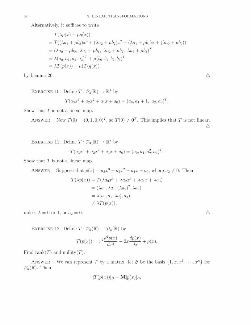
Exercise 10. Define T : P3(R) → R4 by

T (a3x3 + a2x

2 + a1x + a0) = (a0, a1 + 1, a2, a3)T .

Show that T is not a linear map.

Answer. Now T (0) = (0, 1, 0, 0)T , so T (0) �= 0T . This implies that T is not linear.�

Exercise 11. Define T : P3(R) → R∗ by

T (a3x3 + a2x

2 + a1x + a0) = (a0, a1, a22, a3)

T .

Show that T is not a linear map.

Answer. Suppose that p(x) = a3x3 + a2x

2 + a1x + a0, where a2 �= 0. Then

T (λp(x)) = T (λa3x3 + λa2x

2 + λa1x + λa0)

= (λa0, λa1, (λa2)2, λa3)

= λ(a0, a1, λa22, a3)

�= λT (p(x)),

unless λ = 0 or 1, or a2 = 0. �

Exercise 12. Define T : Pn(R) → Pn(R) by

T (p(x)) = x2 d2p(x)

dx2− 2x

dp(x)

dx+ p(x).

Find rank(T ) and nullity(T ).

Answer. We can represent T by a matrix: let B be the basis {1, x, x2, · · · , xn} forPn(R). Then

[T (p(x))]B = M[p(x)]B,

4. RANK AND NULLITY 33

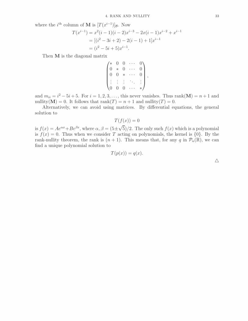
where the ith column of M is [T (xi−1)]B. Now

T (xi−1) = x2(i − 1)(i − 2)xi−3 − 2x(i − 1)xi−2 + xi−1

= [(i2 − 3i + 2) − 2(i − 1) + 1]xi−1

= (i2 − 5i + 5)xi−1.

Then M is the diagonal matrix

∗ 0 0 · · · 00 ∗ 0 · · · 00 0 ∗ · · · 0...

......

. . ....

0 0 0 · · · ∗

,

and mii = i2 − 5i + 5. For i = 1, 2, 3, . . . , this never vanishes. Thus rank(M) = n + 1 andnullity(M) = 0. It follows that rank(T ) = n + 1 and nullity(T ) = 0.

Alternatively, we can avoid using matrices. By differential equations, the generalsolution to

T (f(x)) = 0

is f(x) = Aeαx+Beβx, where α, β = (5±√5)/2. The only such f(x) which is a polynomial

is f(x) = 0. Thus when we consider T acting on polynomials, the kernel is {0}. By therank-nullity theorem, the rank is (n + 1). This means that, for any q in Pn(R), we canfind a unique polynomial solution to

T (p(x)) = q(x).

�