Modelli di FriedmanLezione 7

A. Marconi Cosmologia (2011/2012)

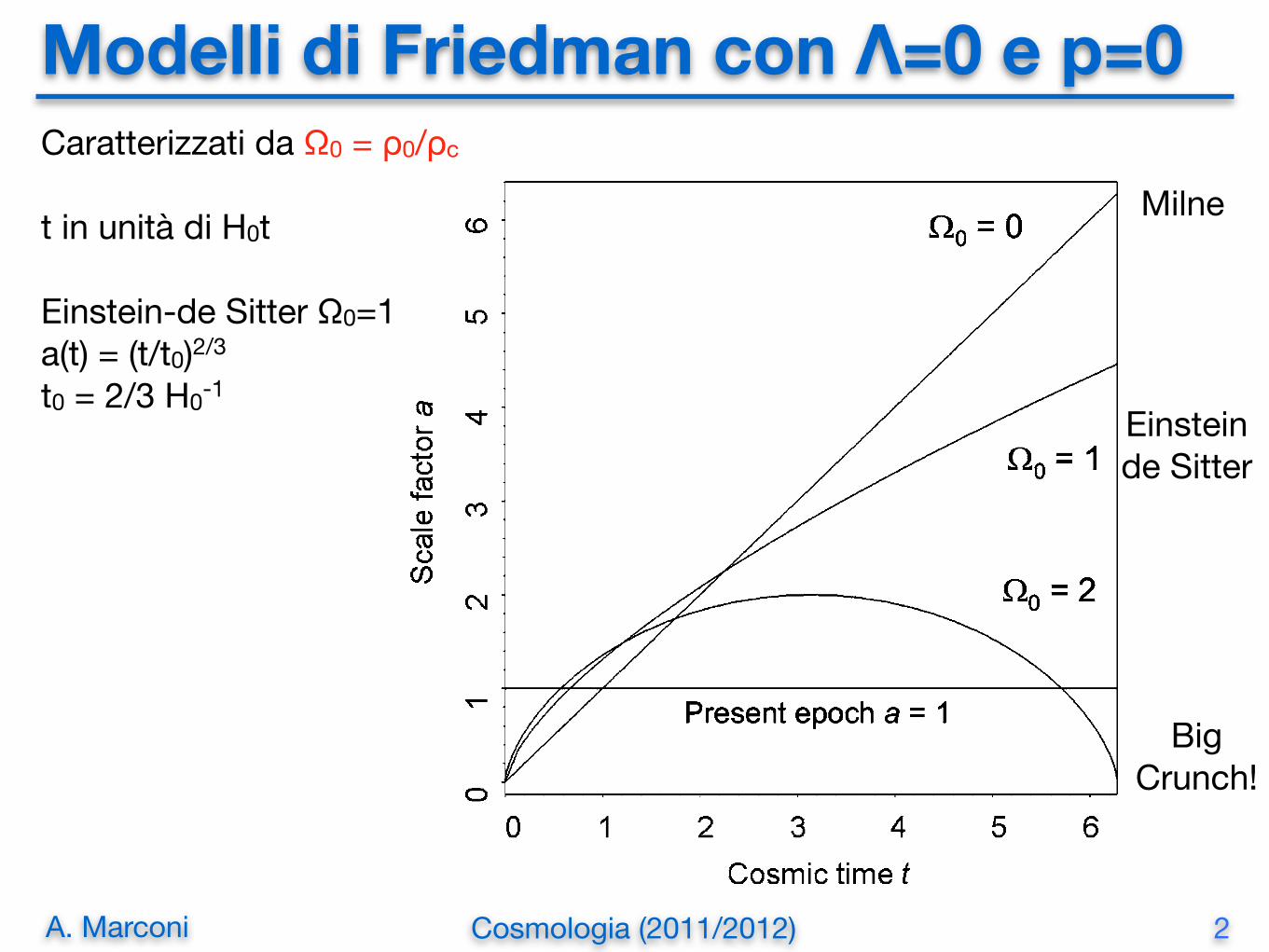
Modelli di Friedman con Λ=0 e p=0Caratterizzati da Ω0 = ρ0/ρc

t in unità di H0t

Einstein-de Sitter Ω0=1 a(t) = (t/t0)2/3

t0 = 2/3 H0-1

2

206 7 The Friedman World Models

to zero as a tends to infinity. It has a particularly simple variation of a(t) withcosmic epoch,

a =!

tt0

"2/3

! = 0, (7.24)

where the present age of the world model is t0 = (2/3)H!10 .

Some solutions of (7.21) are displayed in Fig. 7.2 which shows the well-knownrelation between the dynamics and geometry of the Friedman world models with" = 0. The abscissa in Fig. 7.2 is in units of H!1

0 and so the slope of the relationsat the present epoch, a = 1, is always 1. The present age of the Universe is given bythe intersection of each curve with the line a = 1.

Another useful result is the function a(t) for the empty world model, #0 = 0,a(t) = H0t, ! = !(H0/c)2. This model is sometimes referred to as the Milne

Fig. 7.2. The dynamics of the classical Friedman models with #" = 0 characterised by thedensity parameter #0 = $0/$c. If #0 > 1, the Universe collapses to a = 0 as shown; if#0 < 1, the Universe expands to infinity and has a finite velocity of expansion as a tends toinfinity. In the case #0 = 1, a = (t/t0)2/3 where t0 = (2/3)H!1

0 . The time axis is given interms of the dimensionless time H0t. At the present epoch a = 1 and in this presentation, thethree curves have the same slope of 1 at a = 1, corresponding to a fixed value of Hubble’sconstant at the present day. If t0 is the present age of the Universe, then H0t0 = 1 for #0 = 0,H0t0 = 2/3 for #0 = 1 and H0t0 = 0.57 for #0 = 2

Einsteinde Sitter

Milne

Big Crunch!

A. Marconi Cosmologia (2011/2012)

Modelli di Friedman con Λ>0

3

7.3 Friedman Models with Non-Zero Cosmological Constant 213

Fig. 7.3a–d. Examples of the dynamics of world models in which ! != 0 (Bondi, 1960).Models a and d are referred to as Lemaitre models. In a, the model parameters are "0 = 0.3and "! = 0.7, a favoured model according to current best estimates of these parameters.b This ‘bouncing’ model has "0 = 0.05 and "! = 2. The zero of cosmic time has beenset to the value when a = 0. The loci are symmetrical in cosmic time with respect to thisorigin. c This model is an Eddington–Lemaitre model which is stationary at redshift zc = 3,corresponding to scale factor a = 0.25. In d, the model parameters are "0 = 0.01 and"! = 0.99 and the age of the Universe can far exceed H"1

0

behaviour corresponds to exponentially collapsing and expanding de Sitter solutions

a =!

"! " 1"!

"1/2

exp#±"

1/2! H0#

$. (7.58)

In these ‘bouncing’ Universes, the smallest value of a, amin, corresponds to thelargest redshifts which objects could have.

The most interesting cases are those for which amin # 0. The case where amin = 0is known as the Eddington–Lemaitre model and is illustrated in Fig. 7.3c. The literalinterpretation of these models is either: A, the Universe expanded from an origin atsome finite time in the past and will eventually attain a stationary state in the infinite

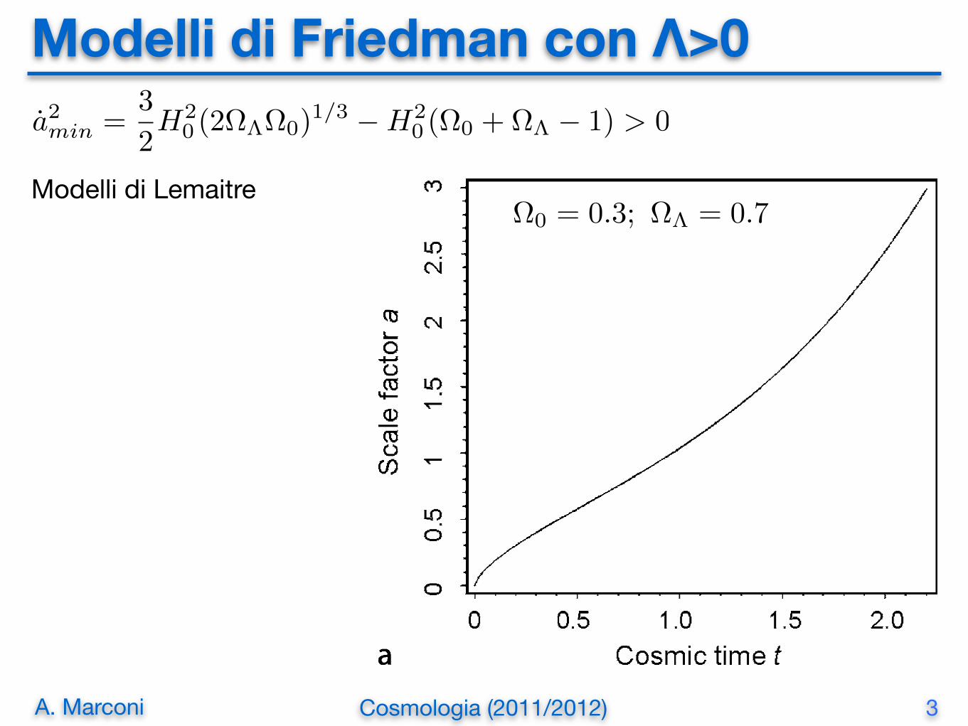
a2min =3

2H2

0 (2⌦⇤⌦0)1/3 �H2

0 (⌦0 + ⌦⇤ � 1) > 0

⌦0 = 0.3; ⌦⇤ = 0.7Modelli di Lemaitre

A. Marconi Cosmologia (2011/2012)

Modelli di Friedman con Λ>0

4

7.3 Friedman Models with Non-Zero Cosmological Constant 213

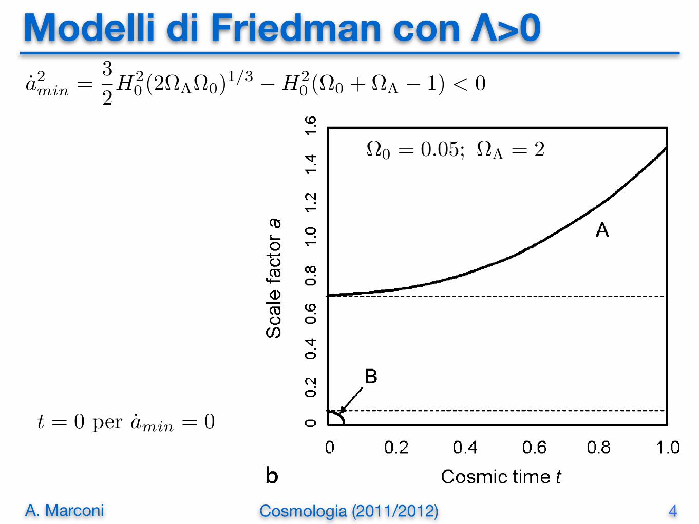
Fig. 7.3a–d. Examples of the dynamics of world models in which ! != 0 (Bondi, 1960).Models a and d are referred to as Lemaitre models. In a, the model parameters are "0 = 0.3and "! = 0.7, a favoured model according to current best estimates of these parameters.b This ‘bouncing’ model has "0 = 0.05 and "! = 2. The zero of cosmic time has beenset to the value when a = 0. The loci are symmetrical in cosmic time with respect to thisorigin. c This model is an Eddington–Lemaitre model which is stationary at redshift zc = 3,corresponding to scale factor a = 0.25. In d, the model parameters are "0 = 0.01 and"! = 0.99 and the age of the Universe can far exceed H"1

0

behaviour corresponds to exponentially collapsing and expanding de Sitter solutions

a =!

"! " 1"!

"1/2

exp#±"

1/2! H0#

$. (7.58)

In these ‘bouncing’ Universes, the smallest value of a, amin, corresponds to thelargest redshifts which objects could have.

The most interesting cases are those for which amin # 0. The case where amin = 0is known as the Eddington–Lemaitre model and is illustrated in Fig. 7.3c. The literalinterpretation of these models is either: A, the Universe expanded from an origin atsome finite time in the past and will eventually attain a stationary state in the infinite

⌦0 = 0.05; ⌦⇤ = 2

a2min =3

2H2

0 (2⌦⇤⌦0)1/3 �H2

0 (⌦0 + ⌦⇤ � 1) < 0

t = 0 per amin = 0

A. Marconi Cosmologia (2011/2012)

Modelli di Friedman con Λ>0

5

7.3 Friedman Models with Non-Zero Cosmological Constant 213

Fig. 7.3a–d. Examples of the dynamics of world models in which ! != 0 (Bondi, 1960).Models a and d are referred to as Lemaitre models. In a, the model parameters are "0 = 0.3and "! = 0.7, a favoured model according to current best estimates of these parameters.b This ‘bouncing’ model has "0 = 0.05 and "! = 2. The zero of cosmic time has beenset to the value when a = 0. The loci are symmetrical in cosmic time with respect to thisorigin. c This model is an Eddington–Lemaitre model which is stationary at redshift zc = 3,corresponding to scale factor a = 0.25. In d, the model parameters are "0 = 0.01 and"! = 0.99 and the age of the Universe can far exceed H"1

0

behaviour corresponds to exponentially collapsing and expanding de Sitter solutions

a =!

"! " 1"!

"1/2

exp#±"

1/2! H0#

$. (7.58)

In these ‘bouncing’ Universes, the smallest value of a, amin, corresponds to thelargest redshifts which objects could have.

The most interesting cases are those for which amin # 0. The case where amin = 0is known as the Eddington–Lemaitre model and is illustrated in Fig. 7.3c. The literalinterpretation of these models is either: A, the Universe expanded from an origin atsome finite time in the past and will eventually attain a stationary state in the infinite

a2min =3

2H2

0 (2⌦⇤⌦0)1/3 �H2

0 (⌦0 + ⌦⇤ � 1) = 0

t = 0 per amin = 0zc = 3

Modelli di Friedman7.4 Observations in Cosmology 215

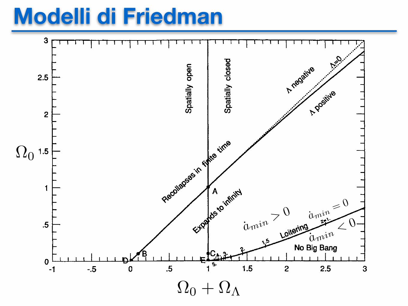
Fig. 7.4. The classification of the Friedman world models with !" != 0 in a plot of !0 against!0 + !" (Carroll et al., 1992). The Eddington–Lemaitre models lie along the line labelled‘loitering’

!" such that the value of amin is just greater than zero. An example of this type ofmodel is shown in Fig. 7.3d.

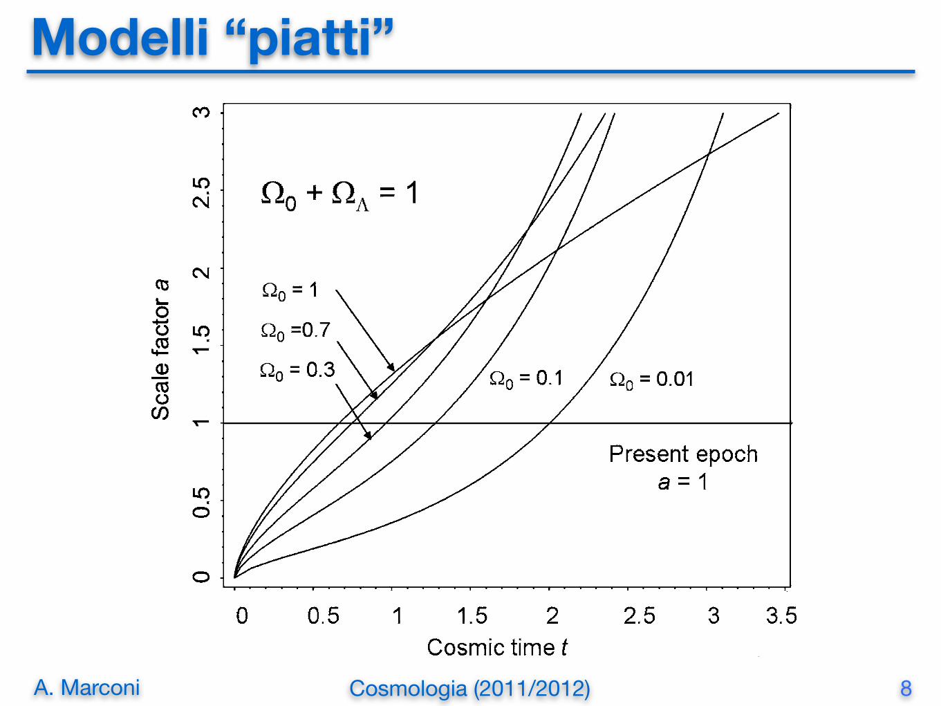
As we will show in Chap. 15, there is now strong evidence that the spatialgeometry of the Universe is flat, so that !0 + !" is very close to unity. Thedynamics of such spatially flat models with different combinations of !0 and !"

are shown in Fig. 7.5. These models indicate how the age of the Universe can begreater than H"1

0 for large enough values of !".

7.4 Observations in Cosmology

Models with finite values of the cosmological constant dominate much of currentcosmological thinking and so it is convenient to develop the expressions for therelations between observables and intrinsic properties in parallel for models withand without the "-term. The reason for including the results for world models with!" = 0 is that they can often be expressed analytically in closed form and so provideinsight into the physics of the world models.

⌦0

⌦0 + ⌦⇤

amin= 0

amin> 0

amin< 0

A. Marconi Cosmologia (2011/2012)

7.3 Friedman Models with Non-Zero Cosmological Constant 213

Fig. 7.3a–d. Examples of the dynamics of world models in which ! != 0 (Bondi, 1960).Models a and d are referred to as Lemaitre models. In a, the model parameters are "0 = 0.3and "! = 0.7, a favoured model according to current best estimates of these parameters.b This ‘bouncing’ model has "0 = 0.05 and "! = 2. The zero of cosmic time has beenset to the value when a = 0. The loci are symmetrical in cosmic time with respect to thisorigin. c This model is an Eddington–Lemaitre model which is stationary at redshift zc = 3,corresponding to scale factor a = 0.25. In d, the model parameters are "0 = 0.01 and"! = 0.99 and the age of the Universe can far exceed H"1

0

behaviour corresponds to exponentially collapsing and expanding de Sitter solutions

a =!

"! " 1"!

"1/2

exp#±"

1/2! H0#

$. (7.58)

In these ‘bouncing’ Universes, the smallest value of a, amin, corresponds to thelargest redshifts which objects could have.

The most interesting cases are those for which amin # 0. The case where amin = 0is known as the Eddington–Lemaitre model and is illustrated in Fig. 7.3c. The literalinterpretation of these models is either: A, the Universe expanded from an origin atsome finite time in the past and will eventually attain a stationary state in the infinite

Modelli di Friedman con Λ>0

7

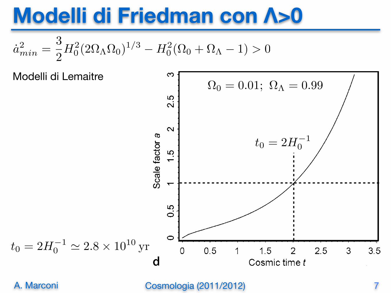
a2min =3

2H2

0 (2⌦⇤⌦0)1/3 �H2

0 (⌦0 + ⌦⇤ � 1) > 0

Modelli di Lemaitre⌦0 = 0.01; ⌦⇤ = 0.99

t0 = 2H�10

t0 = 2H�10 ' 2.8⇥ 1010 yr

A. Marconi Cosmologia (2011/2012)

Modelli “piatti”

8

216 7 The Friedman World Models

Fig. 7.5. The dynamics of spatially flat world models, !0 +!" = 1, with different combina-tions of !0 and !". The abscissa is plotted in units of H!1

0 . The dynamics of these modelscan be compared with those shown in Fig. 7.2 which have !" = 0

7.4.1 The Deceleration Parameter

Just as Hubble’s constant H0 measures the expansion rate of the Universe at thepresent epoch, so we can define the present deceleration of the Universe a(t0). Itis conventional to define the deceleration parameter q0 to be the dimensionlessdeceleration at the present epoch through the expression

q0 = !!

aaa2

"

t0

. (7.61)

Substituting a = 1, a = H0 at the present epoch into the dynamical equation (7.40),we find

q0 = !0

2! !" . (7.62)

Equation (7.62) represents the present competition between the decelerating effectof the attractive force of gravity and the accelerating effect of the repulsive darkenergy. Substituting the favoured values of !0 = 0.3 and !" = 0.7 (see Chaps. 8and 15), we find q0 = !0.55, showing that the Universe is accelerating at the presentepoch because of the dominance of the dark energy.

A. Marconi Cosmologia (2011/2012)

Modelli di Friedman

9

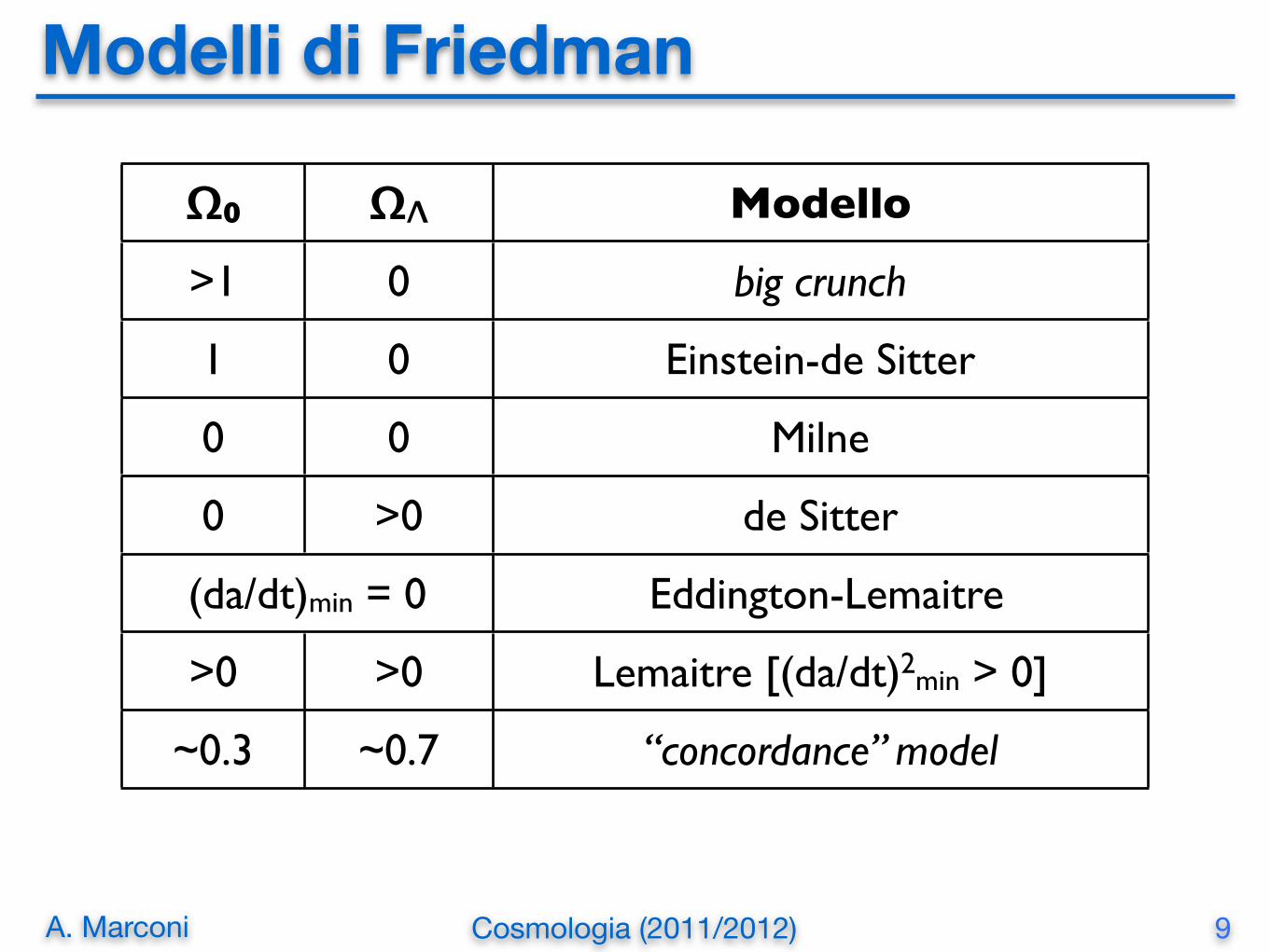
Ω0 ΩΛ Modello

>1 0 big crunch

1 0 Einstein-de Sitter

0 0 Milne

0 >0 de Sitter

(da/dt)min = 0(da/dt)min = 0 Eddington-Lemaitre

>0 >0 Lemaitre [(da/dt)2min > 0]

~0.3 ~0.7 “concordance” model

A. Marconi Cosmologia (2011/2012)

Relazione r-z

10

220 7 The Friedman World Models

r in unità di c/H0

A. Marconi Cosmologia (2011/2012)

Relazione DA-z

11

222 7 The Friedman World Models

Fig. 7.8. a The variation of the angular diameter of a rigid rod of unit proper length withredshift for world models with !" = 0. b The variation of the angular diameter of a rigid rodof unit proper length with redshift for world models with finite values of !" and flat spatialgeometry, !0 + !" = 1. In both diagrams, c/H0 has been set equal to unity

a larger fraction of the celestial sphere at a large redshift, by the factor (1 + z) whichappears in (5.54).

Metric angular diameters are different from the types of angular diameter whichare often used to measure the sizes of galaxies. The latter are often defined to somelimiting surface brightness and so, since bolometric surface brightnesses vary with

Diametro angolare di una stecca rigida di lunghezza unitaria (c/H0=1)

A. Marconi Cosmologia (2011/2012)

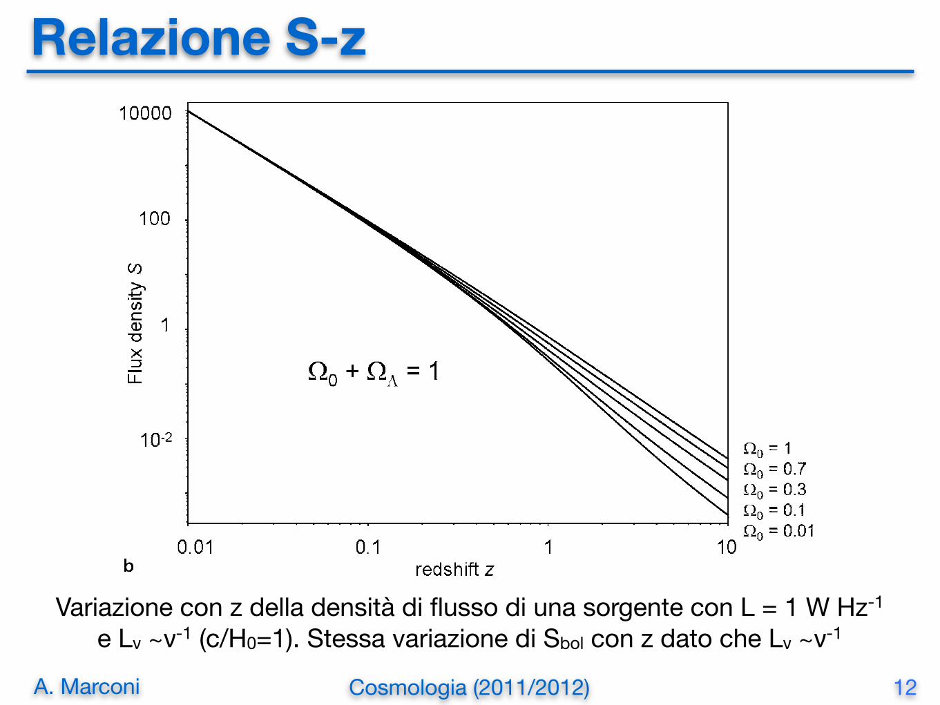
Relazione S-z

12

224 7 The Friedman World Models

Fig. 7.9. The variation of the flux density of a source of luminosity 1 W Hz!1 with a powerlaw spectrum L(!) " !!1 with redshift. In both diagrams, c/H0 = 1. Comparison of (5.65)and (5.66) shows that, since the spectral index " = 1, these relations are the same as thevariations of bolometric flux densities with redshift. a World models with #$ = 0. b Worldmodels with finite values of #$ and flat spatial geometry #0 + #$ = 1

Variazione con z della densità di flusso di una sorgente con L = 1 W Hz-1 e Lν ~ν-1 (c/H0=1). Stessa variazione di Sbol con z dato che Lν ~ν-1

A. Marconi Cosmologia (2011/2012)

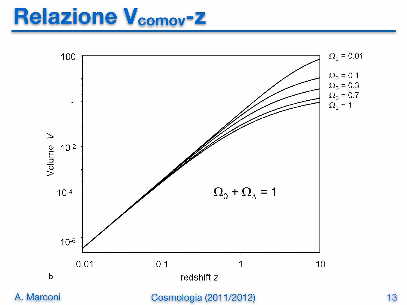
Relazione Vcomov-z

13

7.4 Observations in Cosmology 227

Fig. 7.11. a The variation of the comoving volume within redshift z for world models with!" = 0. b The variation of the comoving volume within redshift z for flat world models withfinite values of !"