LECTURES 20 - 29

INTRODUCTION TOCLASSICAL MECHANICS

Prof. N. Harnew

University of Oxford

HT 2017

1

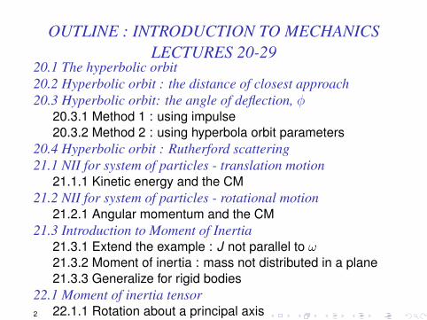
OUTLINE : INTRODUCTION TO MECHANICSLECTURES 20-29

20.1 The hyperbolic orbit20.2 Hyperbolic orbit : the distance of closest approach20.3 Hyperbolic orbit: the angle of deflection, φ

20.3.1 Method 1 : using impulse20.3.2 Method 2 : using hyperbola orbit parameters

20.4 Hyperbolic orbit : Rutherford scattering21.1 NII for system of particles - translation motion

21.1.1 Kinetic energy and the CM21.2 NII for system of particles - rotational motion

21.2.1 Angular momentum and the CM21.3 Introduction to Moment of Inertia

21.3.1 Extend the example : J not parallel to ω21.3.2 Moment of inertia : mass not distributed in a plane21.3.3 Generalize for rigid bodies

22.1 Moment of inertia tensor22.1.1 Rotation about a principal axis2

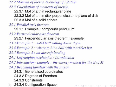
22.2 Moment of inertia & energy of rotation22.3 Calculation of moments of inertia

22.3.1 MoI of a thin rectangular plate22.3.2 MoI of a thin disk perpendicular to plane of disk22.3.3 MoI of a solid sphere

23.1 Parallel axis theorem23.1.1 Example : compound pendulum

23.2 Perpendicular axis theorem23.2.1 Perpendicular axis theorem : example

23.3 Example 1 : solid ball rolling down slope23.4 Example 2 : where to hit a ball with a cricket bat23.5 Example 3 : an aircraft landing24.1 Lagrangian mechanics : Introduction24.2 Introductory example : the energy method for the E of M24.3 Becoming familiar with the jargon

24.3.1 Generalised coordinates24.3.2 Degrees of Freedom24.3.3 Constraints24.3.4 Configuration Space3

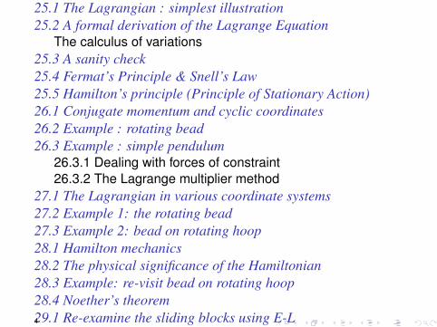
25.1 The Lagrangian : simplest illustration25.2 A formal derivation of the Lagrange Equation

The calculus of variations25.3 A sanity check25.4 Fermat’s Principle & Snell’s Law25.5 Hamilton’s principle (Principle of Stationary Action)26.1 Conjugate momentum and cyclic coordinates26.2 Example : rotating bead26.3 Example : simple pendulum

26.3.1 Dealing with forces of constraint26.3.2 The Lagrange multiplier method

27.1 The Lagrangian in various coordinate systems27.2 Example 1: the rotating bead27.3 Example 2: bead on rotating hoop28.1 Hamilton mechanics28.2 The physical significance of the Hamiltonian28.3 Example: re-visit bead on rotating hoop28.4 Noether’s theorem29.1 Re-examine the sliding blocks using E-L4

29.2 Normal modes of coupled identical springs

29.3 Final example: a rotating coordinate system

5

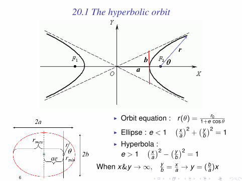
20.1 The hyperbolic orbit

I Orbit equation : r(θ) = r01+e cos θ

I Ellipse : e < 1( x

a

)2+( y

b

)2= 1

I Hyperbola :e > 1

(xa

)2 −(y

b

)2= 1

When x&y →∞, yb = x

a → y = (ba )x

6

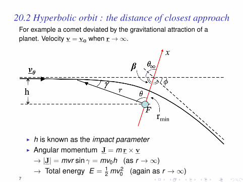
20.2 Hyperbolic orbit : the distance of closest approachFor example a comet deviated by the gravitational attraction of aplanet. Velocity v = v0 when r→∞.

I h is known as the impact parameterI Angular momentum J = m r× v

→ |J| = mvr sin γ = mv0h (as r →∞)→ Total energy E = 1

2 mv20 (again as r →∞)

7

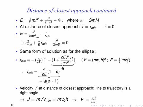
Distance of closest approach continued

I E = 12mr2 + J2

2mr2 − αr , where α = GmM

I At distance of closest approach r = rmin → r = 0I E = J2

2mr2min− α

rmin

→ r2min + α

E rmin − J2

2mE = 0

I Same form of solution as for the ellipse :

I rmin = −(α

2E

)[1− (1 +

2EJ2

mα2 )12︸ ︷︷ ︸

e

] (J2 = (mv0h)2 ; E = 12 mv2

0 )

→ rmin = − α

2E(1− e)︸ ︷︷ ︸

= a(e - 1)I Velocity v ′ at distance of closest approach: line to trajectory is a

right angle.

→ J = mv ′rmin = mv0h → v ′ = v0hrmin

8

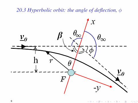
20.3 Hyperbolic orbit: the angle of deflection, φ

9

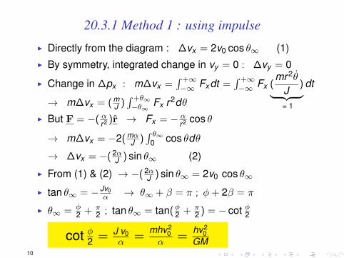
20.3.1 Method 1 : using impulse

I Directly from the diagram : ∆vx = 2v0 cos θ∞ (1)I By symmetry, integrated change in vy = 0 : ∆vy = 0

I Change in ∆px : m∆vx =∫ +∞−∞ Fxdt =

∫ +∞−∞ Fx (

mr2θ

J)︸ ︷︷ ︸

= 1

dt

→ m∆vx = (mJ )∫ +θ∞−θ∞ Fx r2dθ

I But F = −( αr2 )r → Fx = − αr2 cos θ

→ m∆vx = −2(mαJ )∫ θ∞

0 cos θdθ

→ ∆vx = −(2αJ ) sin θ∞ (2)

I From (1) & (2) → −(2αJ ) sin θ∞ = 2v0 cos θ∞

I tan θ∞ = − Jv0α → θ∞ + β = π ; φ+ 2β = π

I θ∞ = φ2 + π

2 ; tan θ∞ = tan(φ2 + π2 ) = − cot φ2

cot φ2 = J v0α =

mhv20

α =hv2

0GM

10

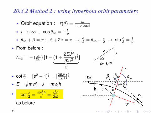
20.3.2 Method 2 : using hyperbola orbit parameters

I Orbit equation : r(θ) = r01+e cos θ

I r → ∞ , cos θ∞ = −1e

I θ∞ + β = π ; φ+ 2β = π → φ2 = θ∞ − π

2 → sin φ2 = 1

e

I From before :

rmin = −(α

2E

)[1− (1 +

2EJ2

mα2 )12︸ ︷︷ ︸

e

]

I cot φ2 = [e2 − 1]12 = [2EJ2

mα2 ]12

I E = 12mv2

0 ; J = mv0h

I cot φ2 =mv2

0 hα =

v20 h

GM

as before

11

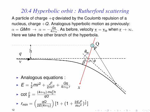
20.4 Hyperbolic orbit : Rutherford scatteringA particle of charge +q deviated by the Coulomb repulsion of anucleus, charge +Q. Analogous hyperbolic motion as previously:α = GMm → α = − Qq

4πε0. As before, velocity v = v0 when r→∞.

Here we take the other branch of the hyperbola.

I Analogous equations :I E = 1

2mr2 + J2

2mr2 + Qq4πε0 r

I cot φ2 =(4πε0)mv2

0 hqQ

I rmin =(

qQ2E(4πε0)

)[1 + (1 + 2EJ2

mα2 )12 ]

12

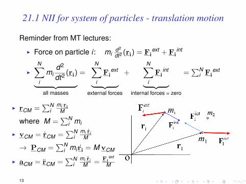
21.1 NII for system of particles - translation motion

Reminder from MT lectures:

I Force on particle i : mid2

dt2 (ri) = Fiext + Fi

int

I

N∑i

mid2

dt2 (ri)︸ ︷︷ ︸all masses

=N∑i

Fiext

︸ ︷︷ ︸external forces

+N∑i

Fiint

︸ ︷︷ ︸internal forces = zero

=∑N

i Fiext

I rCM =∑N

imi ri

M

where M =∑N

i mi

I vCM = rCM =∑N

imi ri

M

→ PCM =∑N

i mi ri = M vCM

I aCM = rCM =∑N

imi ri

M =Fi

ext

M

13

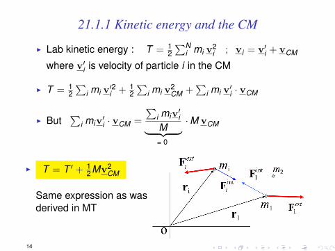
21.1.1 Kinetic energy and the CM

I Lab kinetic energy : T = 12∑N

i mi v2i ; vi = v′i + vCM

where v′i is velocity of particle i in the CM

I T = 12∑

i mi v′2i + 1

2∑

i mi v2CM +

∑i mi v

′i · vCM

I But∑

i miv′i · vCM =

∑i miv

′i

M︸ ︷︷ ︸= 0

·M vCM

I T = T ′ + 12Mv2

CM

Same expression as wasderived in MT

14

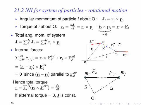
21.2 NII for system of particles - rotational motionI Angular momentum of particle i about O : Ji = ri × pi

I Torque of i about O: τ i =dJidt = ri × pi + ri × pi︸ ︷︷ ︸

= 0

= ri × Fi

I Total ang. mom. of system

J =∑N

i Ji =∑N

i ri × pi

I Internal forces:∑intpair τ (i,j) = ri × Fint

ij + rj × Fintji

= (ri − rj)× Fintij

= 0 since (ri − rj) parallel to Fintij

Hence total torqueτ =

∑Ni (ri × Fext

i ) = dJdt

If external torque = 0,J is const.

15

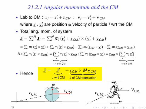
21.2.1 Angular momentum and the CM

I Lab to CM : ri = r′i + rCM ; vi = v′i + vCM

where r′i , v′i are position & velocity of particle i wrt the CM

I Total ang. mom. of system

J =∑N

i Ji =∑N

i mi (r′i + rCM)× (v′i + vCM)

=∑

i mi (r′i ×v′i ) +

∑i mi (r

′i ×vCM) +

∑i mi (rCM ×v′i ) +

∑i mi (rCM ×vCM)

But∑

i mi (r′i × vCM) = [

∑i

mi r′i ]︸ ︷︷ ︸

= 0 in CM

×vCM ;∑

i mi (rCM × v′i ) = rCM × [∑

i

mi v′i ]︸ ︷︷ ︸

= 0 in CM

I HenceJ = J′︸︷︷︸

J wrt CM

+ rCM ×M vCM︸ ︷︷ ︸J of CM translation

16

What we have learned so far

I Newton’s laws relate to rotating systems in the same waythat the laws relate to transitional motion.

I For any system of particles, the rate of change of internalangular momentum about an origin is equal to the totaltorque of the external forces about the origin.

I The total angular momentum about an origin is the sum ofthe total angular momentum about the CM plus the angularmomentum of the translation of the CM.

17

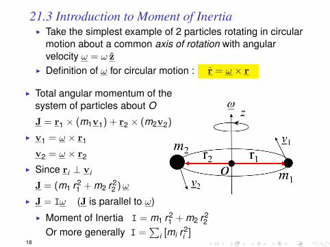
21.3 Introduction to Moment of InertiaI Take the simplest example of 2 particles rotating in circular

motion about a common axis of rotation with angularvelocity ω = ω z

I Definition of ω for circular motion : r = ω × r

I Total angular momentum of thesystem of particles about O

J = r1 × (m1v1) + r2 × (m2v2)

I v1 = ω × r1

v2 = ω × r2

I Since ri ⊥ vi

J = (m1 r21 + m2 r2

2 )ω

I J = Iω (J is parallel to ω)I Moment of Inertia I = m1 r2

1 + m2 r22

Or more generally I =∑

i [mi r2i ]

18

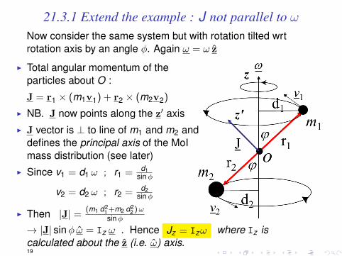
21.3.1 Extend the example : J not parallel to ωNow consider the same system but with rotation tilted wrtrotation axis by an angle φ. Again ω = ω z

I Total angular momentum of theparticles about O :

J = r1 × (m1v1) + r2 × (m2v2)

I NB. J now points along the z′ axisI J vector is ⊥ to line of m1 and m2 and

defines the principal axis of the MoImass distribution (see later)

I Since v1 = d1 ω ; r1 = d1sinφ

v2 = d2 ω ; r2 = d2sinφ

I Then |J| =(m1 d2

1+m2 d22 )ω

sinφ

→ |J| sinφ ω = Iz ω . Hence Jz = Izω where Iz iscalculated about the z (i.e. ω) axis.19

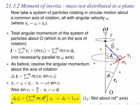
21.3.2 Moment of inertia : mass not distributed in a planeNow take a system of particles rotating in circular motion abouta common axis of rotation, all with angular velocity ω(where vi = ω × ri ).

I Total angular momentum of the system ofparticles about O (which is on the axis ofrotation)

J =∑N

i ri × (mivi) =∑N

i mi rivi ui

(not necessarily parallel to ω axis)I As before, resolve the angular momentum

about the axis of rotation

Jz z =∑N

i mi rivi sinφi ω

I vi = ω × ri ; vi = ωri sinφi

Also sinφi = diri

; vi = ω di

Jz ω =(∑N

i mi d2i

)ω → Jz = Iz ω (Iz : MoI about rotn axis)

20

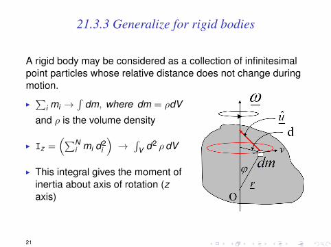
21.3.3 Generalize for rigid bodies

A rigid body may be considered as a collection of infinitesimalpoint particles whose relative distance does not change duringmotion.

I∑

i mi →∫

dm, where dm = ρdV

and ρ is the volume density

I Iz =(∑N

i mi d2i

)→∫

V d2 ρdV

I This integral gives the moment ofinertia about axis of rotation (zaxis)

21

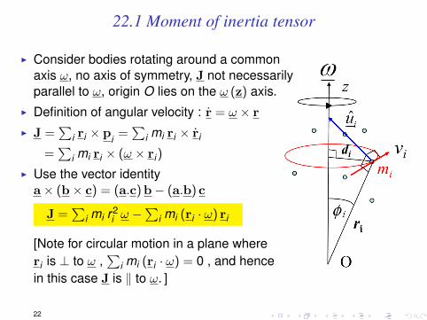
22.1 Moment of inertia tensor

I Consider bodies rotating around a commonaxis ω, no axis of symmetry, J not necessarilyparallel to ω, origin O lies on the ω (z) axis.

I Definition of angular velocity : r = ω × r

I J =∑

i ri × pi =∑

i mi ri × ri

=∑

i mi ri × (ω × ri)

I Use the vector identitya× (b× c) = (a.c)b− (a.b) c

J =∑

i mi r2i ω −

∑i mi (ri · ω) ri

[Note for circular motion in a plane whereri is ⊥ to ω ,

∑i mi (ri · ω) = 0 , and hence

in this case J is ‖ to ω. ]

22

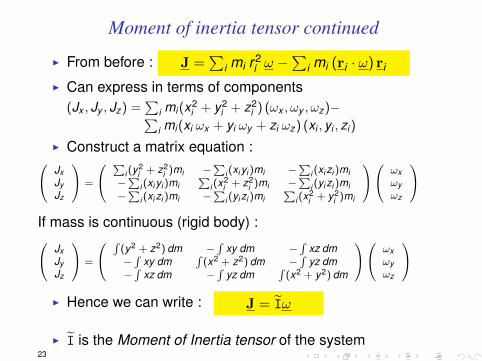
Moment of inertia tensor continued

I From before : J =∑

i mi r2i ω −

∑i mi (ri · ω) ri

I Can express in terms of components(Jx , Jy , Jz) =

∑i mi (x2

i + y2i + z2

i ) (ωx , ωy , ωz)−∑i mi (xi ωx + yi ωy + zi ωz) (xi , yi , zi )

I Construct a matrix equation : JxJyJz

=

∑i (y

2i + z2

i )mi −∑

i (xi yi )mi −∑

i (xi zi )mi−∑

i (xi yi )mi∑

i (x2i + z2

i )mi −∑

i (yi zi )mi−∑

i (xi zi )mi −∑

i (yi zi )mi∑

i (x2i + y2

i )mi

ωxωyωz

If mass is continuous (rigid body) : Jx

JyJz

=

∫(y2 + z2) dm −

∫xy dm −

∫xz dm

−∫

xy dm∫(x2 + z2) dm −

∫yz dm

−∫

xz dm −∫

yz dm∫(x2 + y2) dm

ωxωyωz

I Hence we can write : J = Iω

I I is the Moment of Inertia tensor of the system23

22.1.1 Rotation about a principal axisI In general J = Iω , where I is the Moment of Inertia Tensor Jx

JyJz

=

Ixx Ixy IxzIyx Iyy IyzIzx Izy Izz

ωxωyωz

I Whenever possible, one aligns the axes of the coordinate

system in such a way that the mass of the body evenlydistributes around the axes: we choose axes of symmetry. JxJyJz

=

Ixx 0 00 Iyy 00 0 Izz

ωxωyωz

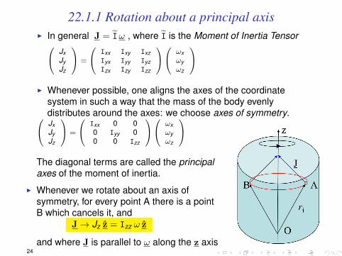
The diagonal terms are called the principalaxes of the moment of inertia.

I Whenever we rotate about an axis ofsymmetry, for every point A there is a pointB which cancels it, and

J→ Jz z = Izz ω z

and where J is parallel to ω along the z axis24

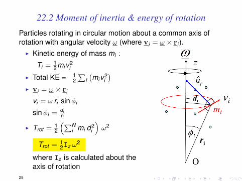
22.2 Moment of inertia & energy of rotation

Particles rotating in circular motion about a common axis ofrotation with angular velocity ω (where vi = ω × ri ).

I Kinetic energy of mass mi :

Ti = 12miv2

i

I Total KE = 12∑

i(miv2

i

)I vi = ω × ri

vi = ω ri sinφi

sinφi = diri

I Trot = 12

(∑Ni mi d2

i

)ω2

Trot = 12Iz ω

2

where Iz is calculated about theaxis of rotation

25

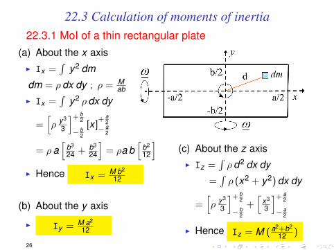
22.3 Calculation of moments of inertia22.3.1 MoI of a thin rectangular plate

(a) About the x axisI Ix =

∫y2 dm

dm = ρdx dy ; ρ = Mab

I Ix =∫

y2 ρdx dy

=[ρ y3

3

]+ b2

− b2

[x ]+ a

2− a

2

= ρa[

b3

24 + b3

24

]= ρa b

[b2

12

]I Hence Ix = M b2

12

(b) About the y axis

I Iy = M a2

12

(c) About the z axisI Iz =

∫ρd2 dx dy

=∫ρ (x2 + y2) dx dy

=[ρ y3

3

]+ b2

− b2

+[

x3

3

]+ a2

− a2

I Hence Iz = M (a2+b2

12 )26

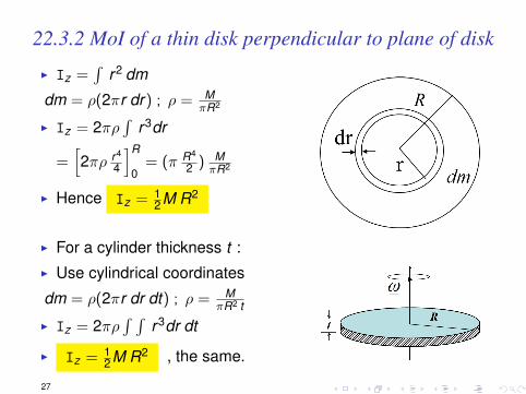
22.3.2 MoI of a thin disk perpendicular to plane of disk

I Iz =∫

r2 dm

dm = ρ(2πr dr) ; ρ = MπR2

I Iz = 2πρ∫

r3dr

=[2πρ r4

4

]R

0= (π R4

2 ) MπR2

I Hence Iz = 12M R2

I For a cylinder thickness t :I Use cylindrical coordinates

dm = ρ(2πr dr dt) ; ρ = MπR2 t

I Iz = 2πρ∫ ∫

r3dr dt

I Iz = 12M R2 , the same.

27

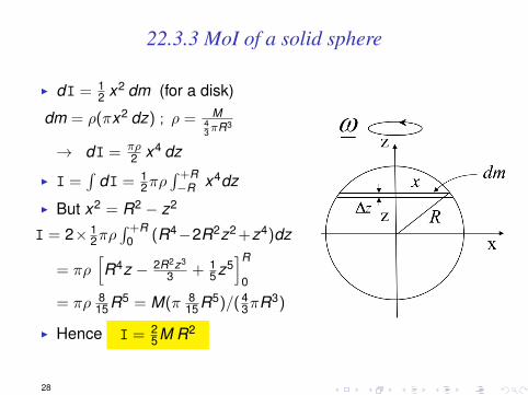
22.3.3 MoI of a solid sphere

I dI = 12 x2 dm (for a disk)

dm = ρ(πx2 dz) ; ρ = M43πR3

→ dI = πρ2 x4 dz

I I =∫

dI = 12πρ

∫ +R−R x4dz

I But x2 = R2 − z2

I = 2× 12πρ

∫ +R0 (R4−2R2z2 +z4)dz

= πρ[R4z − 2R2z3

3 + 15z5]R

0

= πρ 815R5 = M(π 8

15R5)/(43πR3)

I Hence I = 25M R2

28

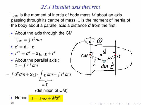
23.1 Parallel axis theoremICM is the moment of inertia of body mass M about an axispassing through its centre of mass. I is the moment of inertia ofthe body about a parallel axis a distance d from the first.

I About the axis through the CM

ICM =∫

r2dmI r′ = d + r

I r ′ 2 = d2 + 2d · r + r2

I About the parallel axis :I =

∫r ′ 2dm

=∫

d2dm + 2d ·∫

rdm︸ ︷︷ ︸= 0

+∫

r2dm

(definition of CM)

I Hence I = ICM + Md2

29

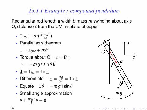
23.1.1 Example : compound pendulum

Rectangular rod length a width b mass m swinging about axisO, distance ` from the CM, in plane of paper

I ICM = m (a2+b2

12 )

I Parallel axis theorem :

I = ICM + m`2

I Torque about O = r× F :

τ = −m g ` sin θ kI J = Iω = I θ k

I Differentiate : τ = dJdt = I θ k

I Equate I θ = −m g ` sin θI Small angle approximation

θ + m g `Iθ = 0

30

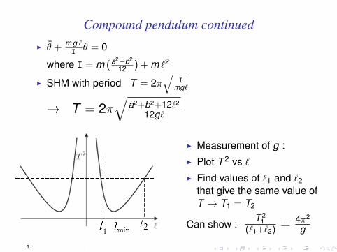
Compound pendulum continued

I θ + m g `Iθ = 0

where I = m (a2+b2

12 ) + m `2

I SHM with period T = 2π√

Img`

→ T = 2π√

a2+b2+12`2

12g`

I Measurement of g :I Plot T 2 vs `I Find values of `1 and `2

that give the same value ofT → T1 = T2

Can show :T 2

1(`1+`2) =

4π2

g

31

23.2 Perpendicular axis theorem

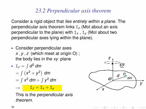
Consider a rigid object that lies entirely within a plane. Theperpendicular axis theorem links Iz (MoI about an axisperpendicular to the plane) with Ix , Iy (MoI about twoperpendicular axes lying within the plane).

I Consider perpendicular axesx , y , z (which meet at origin O) ;the body lies in the xy plane

I Iz =∫

d2 dm

=∫ (

x2 + y2) dm

=∫

x2 dm +∫

y2 dm

→ Iz = Ix + Iy

This is the perpendicular axistheorem.

32

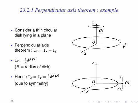
23.2.1 Perpendicular axis theorem : example

I Consider a thin circulardisk lying in a plane

I Perpendicular axistheorem : Iz = Ix + Iy

I Iz = 12M R2

(R = radius of disk)

I Hence Ix = Iy = 14M R2

(due to symmetry)

33

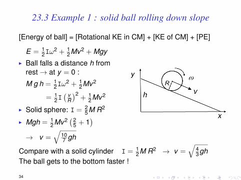
23.3 Example 1 : solid ball rolling down slope

[Energy of ball] = [Rotational KE in CM] + [KE of CM] + [PE]

E = 12Iω

2 + 12Mv2 + Mgy

I Ball falls a distance h fromrest→ at y = 0 :

M g h = 12Iω

2 + 12Mv2

= 12I( v

R

)2+ 1

2Mv2

I Solid sphere: I = 25M R2

I Mgh = 12Mv2 (2

5 + 1)

→ v =√

107 gh

Compare with a solid cylinder I = 12M R2 → v =

√43gh

The ball gets to the bottom faster !

34

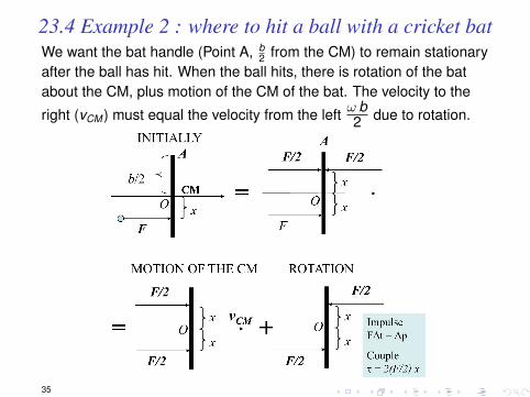
23.4 Example 2 : where to hit a ball with a cricket batWe want the bat handle (Point A, b

2 from the CM) to remain stationaryafter the ball has hit. When the ball hits, there is rotation of the batabout the CM, plus motion of the CM of the bat. The velocity to the

right (vCM ) must equal the velocity from the left ω b2 due to rotation.

35

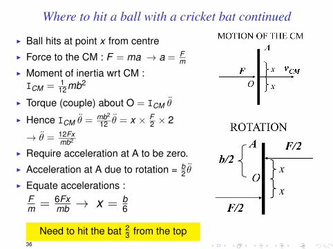
Where to hit a ball with a cricket bat continued

I Ball hits at point x from centreI Force to the CM : F = ma → a = F

mI Moment of inertia wrt CM :ICM = 1

12mb2

I Torque (couple) about O = ICM θ

I Hence ICM θ = mb2

12 θ = x × F2 × 2

→ θ = 12Fxmb2

I Require acceleration at A to be zero.I Acceleration at A due to rotation = b

2 θ

I Equate accelerations :Fm = 6Fx

mb → x = b6

Need to hit the bat 23 from the top

36

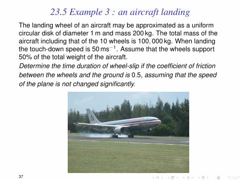
23.5 Example 3 : an aircraft landingThe landing wheel of an aircraft may be approximated as a uniformcircular disk of diameter 1 m and mass 200 kg. The total mass of theaircraft including that of the 10 wheels is 100,000 kg. When landingthe touch-down speed is 50 ms−1. Assume that the wheels support50% of the total weight of the aircraft.Determine the time duration of wheel-slip if the coefficient of frictionbetween the wheels and the ground is 0.5, assuming that the speedof the plane is not changed significantly.

37

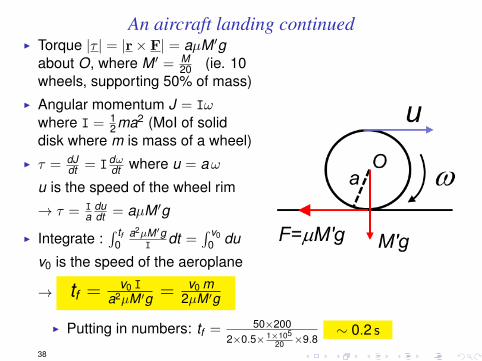
An aircraft landing continuedI Torque |τ | = |r× F| = aµM ′g

about O, where M ′ = M20 (ie. 10

wheels, supporting 50% of mass)I Angular momentum J = Iω

where I = 12ma2 (MoI of solid

disk where m is mass of a wheel)I τ = dJ

dt = Idωdt where u = aω

u is the speed of the wheel rim

→ τ = Ia

dudt = aµM ′g

I Integrate :∫ tf

0a2µM′g

Idt =

∫ v00 du

v0 is the speed of the aeroplane

→ tf = v0 Ia2µM ′g = v0 m

2µM ′g

I Putting in numbers: tf = 50×2002×0.5× 1×105

20 ×9.8∼ 0.2 s

38

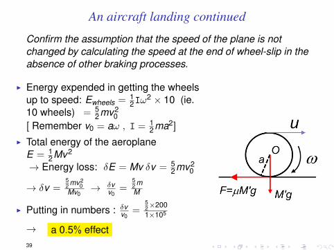
An aircraft landing continued

Confirm the assumption that the speed of the plane is notchanged by calculating the speed at the end of wheel-slip in theabsence of other braking processes.

I Energy expended in getting the wheelsup to speed: Ewheels = 1

2Iω2 × 10 (ie.

10 wheels) = 52mv2

0[ Remember v0 = aω , I = 1

2ma2]

I Total energy of the aeroplaneE = 1

2Mv2

→ Energy loss: δE = Mv δv = 52mv2

0

→ δv =52 mv2

0Mv0

→ δvv0

=52 mM

I Putting in numbers : δvv0

=52×2001×105

→ a 0.5% effect39

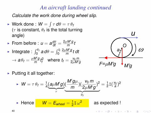
An aircraft landing continuedCalculate the work done during wheel slip.

I Work done : W =∫τ dθ = τ θf

(τ is constant, θf is the total turningangle)

I From before : u = adθdt = 2µM′g

m t

I Integrate :∫ θf

0 a dθ =∫ tf

02µM′g

m t dt

→ a θf = µM′gm t2

f where tf = v0 m2µM′g

I Putting it all together:

I W = τ θf = 1a (aµM ′g)︸ ︷︷ ︸

τ

(M ′gµ

m)(

v0 m2µM ′g

)2︸ ︷︷ ︸θf

= 12I(v0

a )2

I Hence W = Ewheel = 12Iω

2 as expected !

40

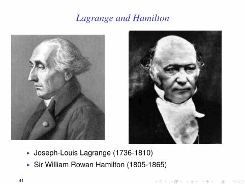
Lagrange and Hamilton

I Joseph-Louis Lagrange (1736-1810)I Sir William Rowan Hamilton (1805-1865)

41

24.1 Lagrangian mechanics : Introduction

I Lagrangian Mechanics: a very effective way to find theequations of motion for complicated dynamical systemsusing a scalar treatment

→ Newton’s laws are vector relations. The Lagrangian is asingle scalar function of the system variables

I Avoid the concept of force

→ For complicated situations, it may be hard to identify allthe forces, especially if there are constraints

I The Lagrangian treatment provides a framework forrelating conservation laws to symmetry

I The ideas may be extended to most areas of fundamentalphysics (special and general relativity, electromagnetism,quantum mechanics, quantum field theory .... )

42

24.2 Introductory example : the energy method for theE of M

I For conservative forces in 1D motion :

Energy of system : E = 12mx2 + U(x) [Note dE

dt = 0]

I Differentiate wrt time: mxx + ∂U∂x x = 0

→ m x = −∂U∂x = F

→ This is the E of M for a conservative forceI Take a simple 1d spring undergoing SHM :

E = 12mx2 + 1

2kx2 = constantdEdt = 0 → mxx + kxx = 0

→ mx + kx = 0I Hence we derived the E of M without using NII directly.

43

24.3 Becoming familiar with the jargon

24.3.1 Generalised coordinates

A set of parameters qk (t) that specifies the systemconfiguration. qk may be a geometrical parameter, x , y , z,a set of angles · · · etc

24.3.2 Degrees of Freedom

The number of degrees of freedom is the number ofindependent coordinates that is sufficient to describe theconfiguration of the system uniquely.

44

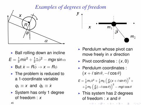
Examples of degrees of freedom

I Ball rolling down an incline

E = 12mx2 + 1

2Iφ2 −mgx sinα

I But x = Rφ→ x = RφI The problem is reduced to

a 1-coordinate variable

q1 ≡ x and q1 ≡ xI System has only 1 degree

of freedom : x

I Pendulum whose pivot canmove freely in x direction

I Pivot coordinates : (x ,0)

I Pendulum coordinates :(x + ` sin θ,−` cos θ)

E = 12 m1x2 + 1

2 m2

(ddt (x + ` sin θ)

)2+

+ 12 m2

(ddt (−` cos θ)

)2−mg` cos θ

I This system has 2 degreesof freedom : x and θ

45

24.3.3 Constraints

I A system has constraints if its components are notpermitted to move freely in 3-D. For example :

→ A particle on a table is restricted to move in 2-D

→ A mass on a simple pendulum is restricted to oscillateat an angle θ at a fixed length ` from a pivot

I The constraints are Holonomic if :

→ The constraints are time independent

→ The system can be described by relations betweengeneral coordinate variables and time

→ The number of general coordinates is reducedto the number of degrees of freedom

46

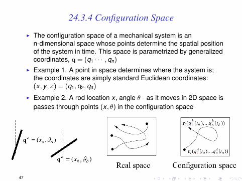
24.3.4 Configuration Space

I The configuration space of a mechanical system is ann-dimensional space whose points determine the spatial positionof the system in time. This space is parametrized by generalizedcoordinates, q = (q1 · · · ,qn)

I Example 1. A point in space determines where the system is;the coordinates are simply standard Euclidean coordinates:(x , y , z) = (q1,q2,q3)

I Example 2. A rod location x , angle θ - as it moves in 2D space ispasses through points (x , θ) in the configuration space

47

25.1 The Lagrangian : simplest illustrationThe Lagrangian : L = T − U

I In 1D : Kinetic energy T = 12 mx2 No explicit dependence on x

Potential energy U = U(x) No explicit dependence on xI Define the Lagrangian in 1D : L = 1

2mx2 − U(x)

I ∂L∂x = mx and ∂L

∂x = −∂U∂x gives force F

I Differentiate wrt time : ddt

(∂L∂x

)= mx = F

I Hence we get the Euler - Lagrange equation for x :ddt

(∂L∂x

)= ∂L

∂x

I Now generalize : the Lagrangian becomes a function of 2nvariables (n is the dimension of the configuration space).Variables are the positions and velocitiesL(q1, · · · ,qn, q1, · · · , qn)

ddt

(∂L∂qk

)= ∂L

∂qkNext we expand on this concept.

48

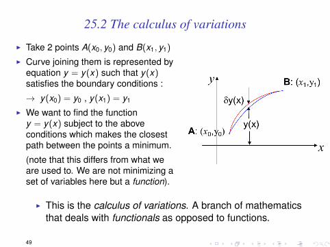
25.2 The calculus of variations

I Take 2 points A(x0, y0) and B(x1, y1)

I Curve joining them is represented byequation y = y(x) such that y(x)satisfies the boundary conditions :

→ y(x0) = y0 , y(x1) = y1

I We want to find the functiony = y(x) subject to the aboveconditions which makes the closestpath between the points a minimum.

(note that this differs from what weare used to. We are not minimizing aset of variables here but a function).

I This is the calculus of variations. A branch of mathematicsthat deals with functionals as opposed to functions.

49

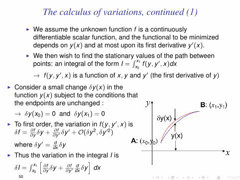
The calculus of variations, continued (1)

I We assume the unknown function f is a continuouslydifferentiable scalar function, and the functional to be minimizeddepends on y(x) and at most upon its first derivative y ′(x).

I We then wish to find the stationary values of the path betweenpoints: an integral of the form I =

∫ x1

x0f (y , y ′, x)dx

→ f (y , y ′, x) is a function of x , y and y ′ (the first derivative of y )

I Consider a small change δy(x) in thefunction y(x) subject to the conditions thatthe endpoints are unchanged :

→ δy(x0) = 0 and δy(x1) = 0I To first order, the variation in f (y , y ′, x) isδf = ∂f

∂y δy + ∂f∂y ′ δy ′ +O(δy2, δy ′2)

where δy ′ = ddx δy

I Thus the variation in the integral I is

δI =∫ x1

x0

[∂f∂y δy + ∂f

∂y ′ddx δy

]dx

50

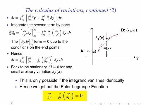
The calculus of variations, continued (2)I δI =

∫ x1

x0

[∂f∂y δy + ∂f

∂y ′ddx δy

]dx

I Integrate the second term by parts∫2ndterm =

[∂f∂y ′ δy

]x1

x0

−∫ x1

x0

ddx

(∂f∂y ′

)δy dx

The[

∂f∂y′ δy

]x1

x0term = 0 due to the

conditions on the end pointsI Hence

δI =∫ x1

x0

[∂f∂y −

ddx

(∂f∂y ′

)]δy dx

I For I to be stationary, δI = 0 for anysmall arbitrary variation δy(x)

I This is only possible if the integrand vanishes identicallyI Hence we get out the Euler-Lagrange Equation

∂f∂y −

ddx

(∂f∂y ′

)= 0

51

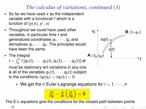
The calculus of variations, continued (3)I So far we have used x as the independent

variable with a functional f which is afunction of (y(x), y ′, x)

I Throughout we could have used othervariables, in particular time t andgeneralized coordinates q1, · · · ,qn andderivatives q1, · · · , qn. The principles wouldhave been the same.

I The integralI =

∫ t1t0

f [q1(t), · · · ,qn(t), q1(t), · · · , qn(t)] dt

must be stationary wrt variations in any one& all of the variables q1(t), · · · ,qn(t) subjectto the conditions δqi (t0) = δqi (t1) = 0

I We get the n Euler-Lagrange equations for i = 1, · · · ,n

∂f∂qi− d

dt

(∂f∂qi

)= 0

The E-L equations give the conditions for the closest path between points52

25.3 A sanity check

The shortest distance between 2 points.

I Consider 2 neighboring points on the curve y(x) subject toboundary conditions y(x0) = y0 , y(x1) = y1

I Distance between the points d` =√

dx2 + dy2

I d` =√

1 + y ′2 dx f ≡√

1 + y ′2

I The Euler-Lagrange Equation ∂f∂y −

ddx

(∂f∂y ′

)= 0

I ∂f∂y = 0 , ∂f

∂y ′ = y ′√1+y ′2

, ddx

(∂f∂y ′

)= 0

I Hence y ′√1+y ′2

= constant, hence y ′ is constant

→ y = mx + cI We have proved that the shortest distance between 2

points is a straight line !

53

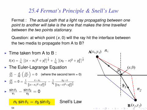
25.4 Fermat’s Principle & Snell’s Law

Fermat : The actual path that a light ray propagating between onepoint to another will take is the one that makes the time travelledbetween the two points stationary.

Question: at which point (x ,0) will the ray hit the interface betweenthe two media to propagate from A to B?

I Time taken from A to B :

t(x) = 1v1

[(x − x1)

2 + y21] 1

2 + 1v2

[(x2 − x)2 + y2

2] 1

2

I The Euler-Lagrange Equation∂t∂x −

ddy

(∂t∂x′

)= 0 (where the second term = 0)

I ∂t∂x = 0 = 1

v1

x−x1

[(x−x1)2+y2

1 ]12− 1

v2

x2−x

[(x2−x)2+y22 ]

12

I sin θ1v1− sin θ2

v2= 0

n1 sin θ1 = n2 sin θ2 Snell’s Law54

25.5 Hamilton’s principle (Principle of Stationary Action)

I Consider for example a particle of mass m at point (xA, yA)moving under the influence of a force in the x − y plane.We want to find the path that the particle will follow toreach a point (xB, yB).

I Hamilton’s principle: the path that the particle will take fromA to B is the one that makes the following functionalstationary :

I =∫ B

A L (q1(t), · · · ,qn(t), q1(t), · · · , qn(t)) dt

where L is the Lagrangian, I is called the action integralI Hence the action integral I is stationary under arbitrary

variations q1(t),q2(t) · · · which vanish at the limits ofintegration ie. A and B.

55

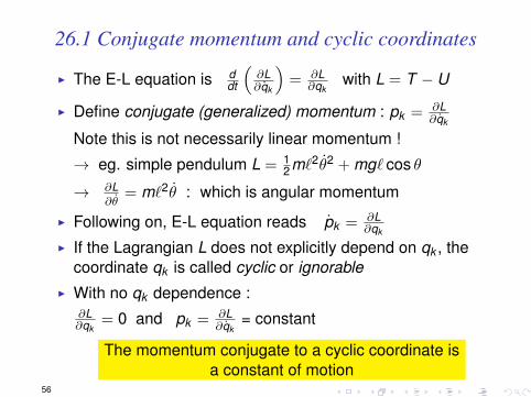
26.1 Conjugate momentum and cyclic coordinates

I The E-L equation is ddt

(∂L∂qk

)= ∂L

∂qkwith L = T − U

I Define conjugate (generalized) momentum : pk = ∂L∂qk

Note this is not necessarily linear momentum !

→ eg. simple pendulum L = 12m`2θ2 + mg` cos θ

→ ∂L∂θ

= m`2θ : which is angular momentum

I Following on, E-L equation reads pk = ∂L∂qk

I If the Lagrangian L does not explicitly depend on qk , thecoordinate qk is called cyclic or ignorable

I With no qk dependence :∂L∂qk

= 0 and pk = ∂L∂qk

= constant

The momentum conjugate to a cyclic coordinate isa constant of motion

56

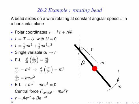
26.2 Example : rotating beadA bead slides on a wire rotating at constant angular speed ω ina horizontal plane

I Polar coordinates v = r r + r θθI L = T − U with U = 0I L = 1

2mr2 + 12mr2ω2

I Single variable qk → r

I E-L ddt

(∂L∂ r

)= ∂L

∂ r

∂L∂ r = mr → d

dt

(∂L∂ r

)= mr

∂L∂r = mrω2

I E-L→ mr −mrω2 = 0

Central force Fcentral = mω2rI r = Aeωt + Be−ωt

57

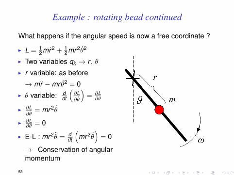
Example : rotating bead continued

What happens if the angular speed is now a free coordinate ?

I L = 12mr2 + 1

2mr2θ2

I Two variables qk → r , θI r variable: as before

→ mr −mr θ2 = 0I θ variable: d

dt

(∂L∂θ

)= ∂L

∂θ

I ∂L∂θ

= mr2θ

I ∂L∂θ = 0

I E-L : mr2θ = ddt

(mr2θ

)= 0

→ Conservation of angularmomentum

58

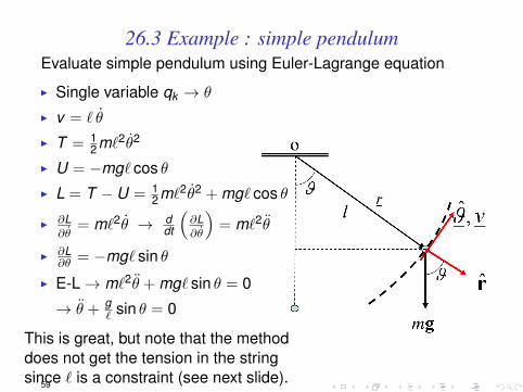
26.3 Example : simple pendulumEvaluate simple pendulum using Euler-Lagrange equation

I Single variable qk → θ

I v = ` θ

I T = 12m`2θ2

I U = −mg` cos θI L = T − U = 1

2m`2θ2 + mg` cos θ

I ∂L∂θ

= m`2θ → ddt

(∂L∂θ

)= m`2θ

I ∂L∂θ = −mg` sin θ

I E-L→ m`2θ + mg` sin θ = 0

→ θ + g` sin θ = 0

This is great, but note that the methoddoes not get the tension in the stringsince ` is a constraint (see next slide).59

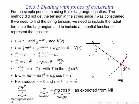
26.3.1 Dealing with forces of constraintFor the simple pendulum using Euler-Lagrange equation. Themethod did not get the tension in the string since ` was constrained.If we need to find the string tension, we need to include the radialterm into the Lagrangian and to include a potential function torepresent the tension:

I `→ r , add 12 mr2 , add V (r)

I L = 12 mr2 + 1

2 mr2θ2 + mgr cos θ − V (r)

I ∂L∂ r = mr → d

dt

(∂L∂ r

)= mr

I ∂L∂r = mr θ2 + mg cos θ − ∂V (r)

∂r

I −∂V (r)∂r = (−T ) with T in the −r dirn.

I E-L→ mr = mr θ2 + mg cos θ − TI Reintroduce r = 0 and r = `; v = r θ

mv2

r︸ ︷︷ ︸Centripetal force

= T︸︷︷︸Tension

−mg cos θ︸ ︷︷ ︸Weight

as expected from NII

60

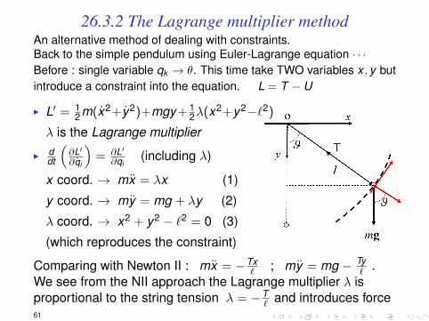
26.3.2 The Lagrange multiplier methodAn alternative method of dealing with constraints.Back to the simple pendulum using Euler-Lagrange equation · · ·Before : single variable qk → θ. This time take TWO variables x , y butintroduce a constraint into the equation. L = T − U

I L′ = 12m(x2+y2)+mgy + 1

2λ(x2+y2−`2)

λ is the Lagrange multiplier

I ddt

(∂L′∂qi

)= ∂L′

∂qi(including λ)

x coord. → mx = λx (1)

y coord. → my = mg + λy (2)

λ coord. → x2 + y2 − `2 = 0 (3)

(which reproduces the constraint)

Comparing with Newton II : mx = −Tx` ; my = mg − Ty

` .We see from the NII approach the Lagrange multiplier λ isproportional to the string tension λ = −T

` and introduces force61

27.1 The Lagrangian in various coordinate systemsI Cartesian coordinates

L = 12 m(x2 + y2 + z2)− U(x , y , z)

Already shown that E-L gives

mx = −∂U∂x ; my = −∂U

∂y ; mz = −∂U∂z

→ m r = −OU

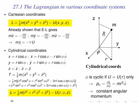
I Cylindrical coordinates

x = r cosφ ; x = r cosφ− r sinφ φ

y = r sinφ ; y = r sinφ+ r cosφ φ

z = z ; z = z

T = 12 m (x2 + y2 + z2)

= 12 m[(r2 cos2 φ+ r2 sin2 φφ2 − 2r r cosφ sinφφ)]

+(r2 sin2 φ+ r2 cos2 φφ2 + 2r r cosφ sinφφ) + z2]

L = 12 m(r2 + r2 φ2 + z2)− U(r , φ, z)

φ is cyclic if U = U(r) only

→ pφ = ∂L∂φ

= mr2φ

→ constant angularmomentum

62

The Lagrangian in various coordinate systems continued

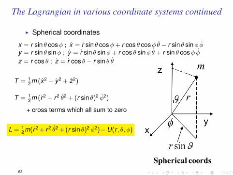
I Spherical coordinates

x = r sin θ cosφ ; x = r sin θ cosφ+ r cos θ cosφ θ − r sin θ sinφ φy = r sin θ sinφ ; y = r sin θ sinφ+ r cos θ sinφ θ + r sin θ cosφ φz = r cos θ ; z = r cos θ − r sin θ θ

T = 12 m (x2 + y2 + z2)

T = 12 m (r2 + r2 θ2 + (r sin θ)2 φ2)

+ cross terms which all sum to zero

L = 12 m(r2 + r2 θ2 + (r sin θ)2 φ2)−U(r , θ, φ)

63

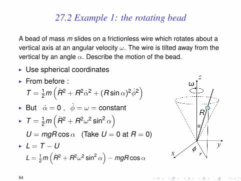
27.2 Example 1: the rotating bead

A bead of mass m slides on a frictionless wire which rotates about avertical axis at an angular velocity ω. The wire is tilted away from thevertical by an angle α. Describe the motion of the bead.

I Use spherical coordinatesI From before :

T = 12m(

R2 + R2α2 + (R sinα)2φ2)

I But α = 0 , φ = ω = constant

I T = 12m(

R2 + R2ω2 sin2 α)

U = mgR cosα (Take U = 0 at R = 0)I L = T − U

L = 12 m(

R2 + R2ω2 sin2 α)−mgR cosα

64

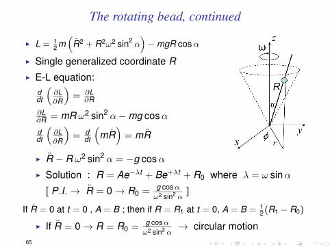
The rotating bead, continued

I L = 12 m(

R2 + R2ω2 sin2 α)−mgR cosα

I Single generalized coordinate RI E-L equation:

ddt

(∂L∂R

)= ∂L

∂R

∂L∂R = mR ω2 sin2 α−mg cosα

ddt

(∂L∂R

)= d

dt

(mR

)= mR

I R − R ω2 sin2 α = −g cosαI Solution : R = Ae−λt + Be+λt + R0 where λ = ω sinα

[ P.I.→ R = 0→ R0 = g cosαω2 sin2 α

]

If R = 0 at t = 0 , A = B ; then if R = R1 at t = 0, A = B = 12 (R1 − R0)

I If R = 0→ R = R0 = g cosαω2 sin2 α

→ circular motion65

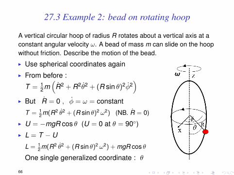
27.3 Example 2: bead on rotating hoop

A vertical circular hoop of radius R rotates about a vertical axis at aconstant angular velocity ω. A bead of mass m can slide on the hoopwithout friction. Describe the motion of the bead.

I Use spherical coordinates againI From before :

T = 12m(

R2 + R2θ2 + (R sin θ)2φ2)

I But R = 0 , φ = ω = constant

T = 12 m(R2 θ2 + (R sin θ)2 ω2) (NB. R = 0)

I U = −mgR cos θ (U = 0 at θ = 90◦)I L = T − U

L = 12 m(R2 θ2 + (R sin θ)2 ω2) + mgR cos θ

One single generalized coordinate : θ

66

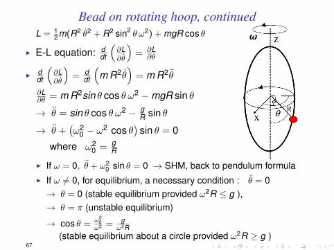
Bead on rotating hoop, continuedL = 1

2 m(R2 θ2 + R2 sin2 θ ω2) + mgR cos θ

I E-L equation: ddt

(∂L∂θ

)= ∂L

∂θ

I ddt

(∂L∂θ

)= d

dt

(m R2θ

)= m R2θ

∂L∂θ = m R2sin θ cos θ ω2 −mgR sin θ

→ θ = sin θ cos θ ω2 − gR sin θ

→ θ +(ω2

0 − ω2 cos θ)

sin θ = 0

where ω20 = g

R

I If ω = 0, θ + ω20 sin θ = 0 → SHM, back to pendulum formula

I If ω 6= 0, for equilibrium, a necessary condition : θ = 0→ θ = 0 (stable equilibrium provided ω2R ≤ g ),→ θ = π (unstable equilibrium)

→ cos θ =ω2

0ω2 = g

ω2R(stable equilibrium about a circle provided ω2R ≥ g )

67

28.1 Hamilton mechanics

I Lagrangian mechanics : Allows us to find the equations ofmotion for a system in terms of an arbitrary set ofgeneralized coordinates

I Now extend the method due to Hamilton→ use of the conjugate (generalized) momentap1,p2, · · · ,pn replace the generalized velocitiesq1, q2, · · · , qn

I This has advantages when some of conjugate momentaare constants of the motion and it is well suited to findingconserved quantities

I From before, conjugate momentum : pk = ∂L∂qk

and E-L equation reads for coordinate k : pk = ∂L∂qk

(since E-L is pk = ddt ( ∂L

∂qk) = ∂L

∂qk)

68

The Hamiltonian, continued

I Lagrangian L = L(qk , qk , t) =⇒

I dLdt = ∂L

∂t +∑

k

(∂L∂qk

dqkdt + ∂L

∂qk

dqkdt

)= ∂L

∂t +∑

k ( ∂L∂qk

qk + ∂L∂qk

qk )

I An aside: use rules ofpartial differentiation:

I If f = f (x , y , z)

I dfdx = ∂f

∂x + ∂f∂y

dydx + ∂f

∂zdzdx

I Conjugate momentum definition : pk = ∂L∂qk

, pk = ∂L∂qk

I Therefore dLdt = ∂L

∂t +∑

k (pk qk + pk qk︸ ︷︷ ︸ddt (pk qk )

)

I ddt (L−

∑k

pk qk︸ ︷︷ ︸- H

) = ∂L∂t

dHdt = −∂L

∂t

I Define Hamiltonian H =∑

k pk qk − LI If L does not depend explicitly on time, H is a constant of motion

69

28.2 The physical significance of the HamiltonianI From before : H =

∑k pk qk − L

I Where conjugate momentum : pk = ∂L∂qk

, pk = ∂L∂qk

I Take kinetic energy T = 12m(x2 + y2 + z2)

I L = 12m(x2 + y2 + z2)− U(x , y , z)

I H =∑

k pk qk − L = 12m (2x .x + 2y .y + 2z.z)− (T − U)

= 2T − (T − U) = T + U = E → total energy

I From before dHdt = −∂L

∂t

→ If L does not depend explicitly on time dHdt = 0

→ energy is a constant of the motion

I Can show by differentiation :Hamilton Equations → ∂H

∂pk= qk ; ∂H

∂qk= −pk

If a coordinate does not appear in the Hamiltonian it iscyclic or ignorable

70

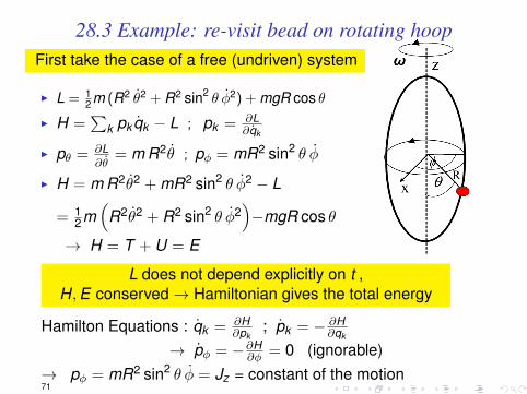
28.3 Example: re-visit bead on rotating hoopFirst take the case of a free (undriven) system

I L = 12 m (R2 θ2 + R2 sin2 θ φ2) + mgR cos θ

I H =∑

k pk qk − L ; pk = ∂L∂qk

I pθ = ∂L∂θ

= m R2θ ; pφ = mR2 sin2 θ φ

I H = m R2θ2 + mR2 sin2 θ φ2 − L

= 12m(

R2θ2 + R2 sin2 θ φ2)−mgR cos θ

→ H = T + U = E

L does not depend explicitly on t ,H,E conserved→ Hamiltonian gives the total energy

Hamilton Equations : qk = ∂H∂pk

; pk = − ∂H∂qk

→ pφ = −∂H∂φ = 0 (ignorable)

→ pφ = mR2 sin2 θ φ = Jz = constant of the motion71

Example continued

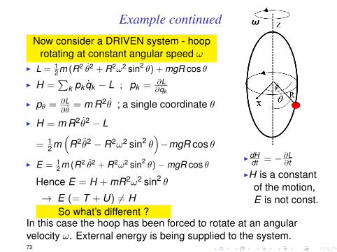
Now consider a DRIVEN system - hooprotating at constant angular speed ω

I L = 12 m (R2 θ2 + R2ω2 sin2 θ) + mgR cos θ

I H =∑

k pk qk − L ; pk = ∂L∂qk

I pθ = ∂L∂θ

= m R2θ ; a single coordinate θ

I H = m R2θ2 − L

= 12m(

R2θ2 − R2ω2 sin2 θ)−mgR cos θ

I E = 12 m (R2 θ2 + R2ω2 sin2 θ)−mgR cos θ

Hence E = H + mR2ω2 sin2 θ

→ E (= T + U) 6= HSo what’s different ?

IdHdt = −∂L

∂tIH is a constant

of the motion,E is not const.

In this case the hoop has been forced to rotate at an angularvelocity ω. External energy is being supplied to the system.72

28.4 Noether’s theoremThe theorem states : Whenever there is a continuous symmetry ofthe Lagrangian, there is an associated conservation law.

I Symmetry means a transformation of the generalizedcoordinates qk and qk that leaves the value of the Lagrangianunchanged.

I If a Lagrangian does not depend on a coordinate qk (ie. is cyclic)it is invariant (symmetric) under changes qk → qk + δqk ; thecorresponding generalized momentum pk = ∂L

∂qkis conserved

1. For a Lagrangian that is symmetric under changes t → t + δt ,the total energy H is conserved→ H =

∑k∂L∂q q− L

2. For a Lagrangian that is symmetric under changes r → r + δr ,the linear momentum p is conserved

3. For a Lagrangian that is symmetric under small rotations ofangle θ → θ + δθ about an axis n such a rotation transforms theCartesian coordinates by r→ r + δθ n× r , the conservedquantity is the component of the angular momentum J along then axis

73

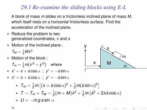
29.1 Re-examine the sliding blocks using E-LA block of mass m slides on a frictionless inclined plane of mass M,which itself rests on a horizontal frictionless surface. Find theacceleration of the inclined plane.

I Reduce the problem to twogeneralized coordinates, x and s

I Motion of the inclined plane :

TM = 12 Mx2

I Motion of the block :

Tm = 12 m(x ′2 + y ′2) where

I x ′ = x + s cosα ; y ′ = −s sinαI x ′ = x + s cosα ; y ′ = −s sinα

I Tm = 12m[(x + s cosα)2 + 1

2m(s sinα)2]I T = Tm + TM = 1

2(m + M)x2 + 12m(s2 + 2x s cosα

)I U = −m g s sin α

74

Sliding blocks, continuedI Lagrangian L = T − UI L = 1

2(m + M)x2 + 12m(s2 + 2x s cosα

)+ mgs sinα

I 2 generalized coordinates → x and s

I The E-L equation ∂L∂qk− d

dt

(∂L∂qk

)= 0

I E-L for x : ∂L∂x = 0 ; d

dt

(∂L∂x

)= d

dt [(m + M)x + ms cosα]

→ (m + M)x + ms cosα = 0 (1)

I E-L for s : ∂L∂s = mg sinα ; d

dt

(∂L∂s

)= d

dt [m (s + x cosα)]

→ s + x cosα = g sinα (2)I Rearranging (1) & (2)

x = −g sinα cosαsin2 α+M/m

; s = g sinα(1+M/m)

sin2 α+M/m

I From (1) Mx + m(x + s cosα) = const.→ Mx + mx ′ = const. Conservation of momentum.

75

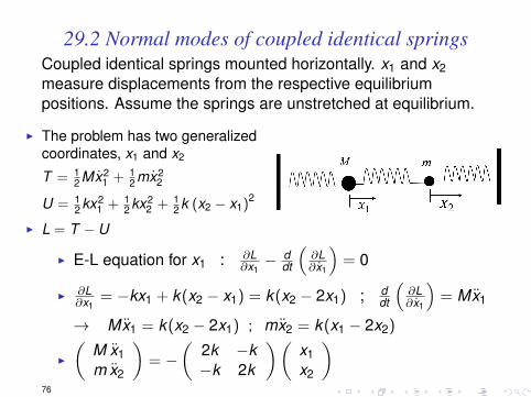
29.2 Normal modes of coupled identical springsCoupled identical springs mounted horizontally. x1 and x2measure displacements from the respective equilibriumpositions. Assume the springs are unstretched at equilibrium.

I The problem has two generalizedcoordinates, x1 and x2

T = 12 Mx2

1 + 12 mx2

2

U = 12 kx2

1 + 12 kx2

2 + 12 k (x2 − x1)2

I L = T − U

I E-L equation for x1 : ∂L∂x1− d

dt

(∂L∂x1

)= 0

I ∂L∂x1

= −kx1 + k(x2 − x1) = k(x2 − 2x1) ; ddt

(∂L∂x1

)= Mx1

→ Mx1 = k(x2 − 2x1) ; mx2 = k(x1 − 2x2)

I

(M x1m x2

)= −

(2k −k−k 2k

)(x1x2

)76

Coupled identical springs, continued

I

(M x1m x2

)= −

(2k −k−k 2k

)(x1x2

)(1)

I SHM solutions(

x1x2

)=

(a1a2

)exp( i ω t)

I Substitute into (1)

−ω2(

M 00 m

)︸ ︷︷ ︸

M

(a1a2

)= −

(2k −k−k 2k

)︸ ︷︷ ︸

K

(a1a2

)

I Putting ω2 = λ → M−1K

(a1a2

)= λ

(a1a2

)I Eigenvalue equation; homogeneous solutionsI Etc etc ....

77

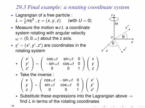
29.3 Final example: a rotating coordinate systemI Lagrangian of a free particle :

L = 12mr2 , r = (x , y , z) (with U = 0)

I Measure the motion w.r.t. a coordinatesystem rotating with angular velocityω = (0,0, ω) about the z axis.

I r′ = (x ′, y ′, z ′) are coordinates in therotating system

I

x ′

y ′

z ′

=

cosωt sinωt 0− sinωt cosωt 0

0 0 1

xyz

I Take the inverse : x

yz

=

cosωt − sinωt 0sinωt cosωt 0

0 0 1

x ′

y ′

z ′

I Substitute these expressions into the Lagrangian above→

find L in terms of the rotating coordinates78

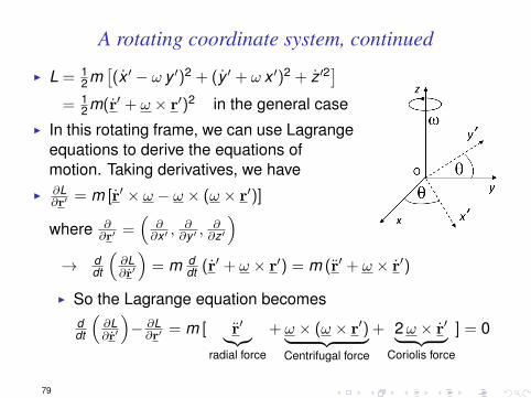
A rotating coordinate system, continued

I L = 12m[(x ′ − ω y ′)2 + (y ′ + ω x ′)2 + z ′2

]= 1

2m(r′ + ω × r′)2 in the general caseI In this rotating frame, we can use Lagrange

equations to derive the equations ofmotion. Taking derivatives, we have

I ∂L∂r′ = m [r′ × ω − ω × (ω × r′)]

where ∂∂r′ =

(∂∂x ′ ,

∂∂y ′ ,

∂∂z′

)→ d

dt

(∂L∂r′

)= m d

dt (r′ + ω × r′) = m (r′ + ω × r′)

I So the Lagrange equation becomesddt

(∂L∂r′

)− ∂L∂r′ = m [ r′︸︷︷︸

radial force

+ ω × (ω × r′)︸ ︷︷ ︸Centrifugal force

+ 2ω × r′︸ ︷︷ ︸Coriolis force

] = 0

79

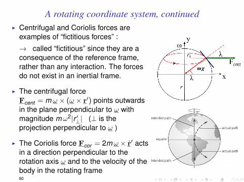
A rotating coordinate system, continuedI Centrifugal and Coriolis forces are

examples of “fictitious forces” :

→ called “fictitious” since they are aconsequence of the reference frame,rather than any interaction. The forcesdo not exist in an inertial frame.

I The centrifugal forceFcent = mω × (ω × r′) points outwardsin the plane perpendicular to ω withmagnitude mω2|r ′⊥| (⊥ is theprojection perpendicular to ω )

I The Coriolis force Fcor = 2mω × r′ actsin a direction perpendicular to therotation axis ω and to the velocity of thebody in the rotating frame80

A rotating coordinate system, continued

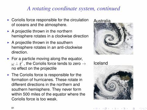
I Coriolis force responsible for the circulationof oceans and the atmosphere.

I A projectile thrown in the northernhemisphere rotates in a clockwise direction

I A projectile thrown in the southernhemisphere rotates in an anti-clockwisedirection.

I For a particle moving along the equator,ω ⊥ r′ , the Coriolis force tends to zero→no effect on the projectile

I The Coriolis force is responsible for theformation of hurricanes. These rotate indifferent directions in the northern andsouthern hemisphere. They never formwithin 500 miles of the equator where theCoriolis force is too weak.

Australia

Iceland

81

THE END

82