Lecture notes in Solid State 3

Eytan Grosfeld

Physics Department, Ben-Gurion University of the Negev

Classical free electron model for metals: The Drude model

Recommended reading:

• Chapter 1, Ashcroft & Mermin.

The conductivity of metals is described very well by the classical Drude formula,

σD =ne2τ

m(1.1)

where m is the electronic mass (as decided by the band-structure) and e is theelectronic charge. The conductivity is directly proportional to the electronicdensity n; and, to τ , the mean free time between collisions of the conductingelectrons with defects that are generically present in the system:

• Static defects that scatter the electron elastically, including: static impu-rities and structural defects. One can dene the elastic mean free timeτe.

• Dynamical defects which scatter the electron inelastically (as they cancarry o energy) including: photons, other electrons, other excitations(such as plasmons). One can accordingly dene the inelastic mean freetime τϕ.

The eciency of the latter processes depends on the temperature T : we expect itto increase as T is increased. At very low temperatures the dominant scatteringis elastic, and then τ does not depend strongly on temperature but instead itdepends on the amount of disorder (realized as random static impurities). Weexpect τ to decrease as the temperature or the amount of disorder in the systemare increased.

The Drude model

1897 - discovery of the electron (J. J. Thomson). 1900 - only three years later,Drude applied the kinetic theory of gases to a metal - considering it to be a gasof electrons. Assumptions:

1. Electrons are classical objects: solid spheres of identical shape.

2. There is a compensating positive charge attached to immobile particles,to ensure overall charge neutrality:

1

2

(a) Each isolated atom of the metallic element has a nucleus of chargeeZa (0 < e = 1.60× 10−19C, Za is the atomic number).

(b) Surrounding the nucleus are Za electrons of total charge −eZa, com-posed of Z weakly bound valence electrons, and Za−Z tightly boundelectrons, the core electrons. In a metal, the core electrons remainbound to the nucleus and form the (immobile, positively charged)metallic ion, while the (mobile, negatively charged) valence electronsare allowed to wander far away from the parent atom. In this contextthey are called the conduction electrons.

3. Electrons are almost free (no forces act between electrons), except elec-trons can collide with ions (more generally, and more correctly, we needonly assume that there is some scattering mechanism, as modern theoriesshow that static ions on a perfectly ordered lattice do not lead to scatter-ing. We will see that later when we discuss Bloch theorem). Between colli-sions they move as dictated by Newton's laws of motion. Electron-electroninteractions are neglected between collisions (independent electron approximation).Electron-ion interactions are neglected as well (free electron approximation).

Many of the properties of metals can be described using the classical Drudetheory, including

• Conductivity,

• Conductivity at nite magnetic eld and Hall conductivity,

• Thermal conductivity (and the historic explanation of the Wiedemann-Franz law which agrees with experimental results: only about a factor of2 too small compared to them),

• Thermoelectric eects (Seebeck eect),

• AC conductivity,

• Interaction with the electromagnetic eld (reection below the plasmafrequency, transmission above the plasma frequency, plasma oscillationsat the plasma frequency).

While many of the results turn out to be inaccurate and the mechanism forscattering remains unexplained, the basic assumption of a free electrons gasthat undergoes scattering remains essentially the same in modern theories.

The modied Newton-like equation describing the average momentum for anelectron can be derived in the following way. An electron experiences a collisionwith a probability per unit time of 1/τ , where τ is known as the relaxationtime or the mean free time. So the probability for a collision in a time intervaldt is dt/τ , and this is also the fraction of electrons that collided during thattime. For a macroscopic number of electrons that have collided, the averagemomentum immediately following the collision is zero. The average momentumfor the electrons at time t+ dt is therefore

p(t+ dt) =dt

τ[0 + F(t)dt]︸ ︷︷ ︸

electrons that collided

+

(1− dt

τ

)[p(t) + F(t)dt]︸ ︷︷ ︸

electrons that did not collide

,(1.2)

3

where p(t) is the momentum per electron, F(t) is the external force per electron.Therefore,

p(t+ dt)− p(t) = F(t)dt− p(t)

τdt+O(dt)2, (1.3)

and we get the central equation of motion for the Drude model

dp

dt= −p(t)

τ+ F(t). (1.4)

Hence the eect of individual electron collisions is to introduce a frictional damp-ing term to the equation of motion.

In more technical terms, following a collision, we will use the Boltzmanndistribution to generate a velocity for the electrons

f(v) =

(m

2πkBT

)3/2

exp

[− mv2

2kBT

](1.5)

so the electrons have an averge speed which is controlled by the (local) temper-ature, but the average velocity is zero due to the angular averaging.

Conductivity

Ohm's law: the current I owing in a wire is proportional to the potential dropV along the wire

V = IR, (1.6)

where R is the resistance (measured in Ohms) which depends on the shape ofthe wire. One can dene the resistivity ρ according to

E = ρj, (1.7)

where E is the electric eld and j is the current density. The quantities arerelated in the following way. For a current owing in a wire of length L andcross-sectional area A the current density along the wire is j = I/A. SinceV = EL, we get V = (ρI/A)L hence

R = ρL/A. (1.8)

All the dependence of R on the dimensions of the wire is now explicit, hence ρis a material property. The inverse resistivity is the conductivity σ = ρ−1. Theinverse resistance is the conductance G (measured in 1/Ohms).

In the framework of the Drude model, we can solve explicitly the dierentialequation with F = −eE, to get

p(t) = −eτE + (p0 + eτE)e−t/τ (1.9)

when t→∞ we reach steady state, for which we get a drift velocity

v = −eEτm

, (1.10)

and a corresponding current density is

j = −nev =ne2τ

mE, σD =

ne2τ

m, (1.11)

justifying Eq. (1.1).

4

Thermal conductivity

The Drude model was able to give an explanation to the empirical law of Wiede-mann and Franz (1853), that the ratio of the thermal to electrical conductivity isdirectly proportional to the temperature, with a proportionality constant whichis more or less the same for all metals. Hence, one denes the ratio κ/σT , knownas the Lorenz number. To estimate the thermal conducitivity of electrons oneconsiders a metal bar along which the temperature varies slowly. Fourier's lawstates that

jq = −κ∇T (1.12)

where jq is the thermal current density (its magnitude is the thermal energy perunit time crossing a unit area perpendicular to the ow). Electrons arriving atpoint r with velocity v have on average underwent a collision at r−vτ and willcarry thermal energy E[T (r− vτ)], hence

jq = −1

2nv E[T (x− vτ)]− E[T (x + vτ)] (1.13)

' −τvn∂E∂T

v · (∇T ) (1.14)

Averaging, we get

〈vv〉 =1

3〈v2〉I (1.15)

and dening

cV = ndE

dT=

3

2nkB (1.16)

we arrive at the result

κ =1

3cV τ〈v2〉 (1.17)

The Lorenz number is

L =κ

σT=

1

3

cV 〈mv2〉ne2T

(1.18)

with 〈mv2〉 = 3kBT one gets

L =3

2

(kBe

)2

= 1.11× 10−8 (J/CK)2

(1.19)

Quantum free electron model for metals: The Sommerfeldmodel

Recommended reading:

• Chapter 2, Aschroft & Mermin.

A quantum model: a free electron gas. At thermal equilibrium, the number ofelectrons having energy E is given by the Fermi distribution

f(E) =1

eβ(E−µ) + 1, (1.20)

in which β = 1/(kBT ) is the inverse temperature (kB is the Boltzmann constant)and µ is the chemical potential. At zero temperature (β → ∞) the chemical

5

potential is equal to the Fermi energy, EF , and the Fermi function describes astep-function, such that all states with energy E ≤ EF are full and all stateswith energy about EF are empty. In the grand-canonical ensemble, where thechemical potential is xed, the number of electrons is temperature-dependent.The electronic density (number of electrons per unit volume) is given by

n =

ˆ ∞−∞

dEN (E)f(E), (1.21)

where N (E) is the density of states (number of states having energy E per unitvolume).

We can straightforwardly adopt the results of the Drude model for this case,however, we need to correct the following points:

• The typical velocity squared for the electrons, 〈v2〉, is set by the Fermienergy and not by the temperature⟨

mv2

2

⟩= EF , (1.22)

(compare with⟨mv2

2

⟩= 3

2kBT for the Boltzmann distribution).

• The electronic heat capacity is proportional to the temperature and isnot a constant. The reason is that at nite temperature T there are∼ Ω(EF )kBT electrons which become excited (here Ω(EF ) ∼ n/EF isthe density of states at the Fermi energy), and they each typically carryadditional energy kBT , leading to an increase in energy of about E ∼Ω(EF )(kBT )2 compared to the ground state; Hence cV ∝ dE

dT ∝ T .

By using equilibrium results to calculate the various physical quantities, onecan adopt the results from the Drude theory after the following corrections:

• cV → cV

(kBTEF

),

•⟨mv2

2

⟩→⟨mv2

2

⟩(EFkBT

).

Hence, since L is proportional to the product, it remains about the same, whileQ gets reduced by a factor of kBT/EF to about 1% of its classical value. Anexact calculation within the Sommerfeld model (using a Sommerfeld expansion,see chapter 2 Ashcroft & Mermin) leads to

L =π2

3

(kBe

)2

= 2.44× 10−8 (J/CK)2, (1.23)

which is an excellent match with the typical experimental value of L.A semiclassical way to calculate directly transport coecients in the Som-

merfeld model is provided by the Boltzmann equation, that extends Sommer-feld's equilibrium theory to nonequilibrium cases.

6

Introduction to Localization

Plan

• Single spatially separated atoms: electrons are localized near atoms.

• Clean crystal: tunneling between perfectly ordered atoms→ Bloch theorem→ extended electronic eigenstates.

• What happens if we add disorder?

The Anderson model

Tight-binding in the presence of on-site disorder

H =∑i

εi|i〉〈i|+ t∑〈ij〉

|i〉〈j| (1.24)

andεi ∈ [−W/2,W/2] (1.25)

randomly and uniformly chosen, where W is the disorder strength,

εi = 0 (1.26)

εiεj =W 2

12δij (1.27)

In the presence of magnetic eld

H =∑i

εi|i〉〈i|+ t∑〈ij〉

eiθij |i〉〈j| (1.28)

where θij = − e~c´ jiA · d`, known as the Peierls substitution.

The Anderson model - implications for transport

Localized states decay away from their center, i.e. behave asymptotically like

ψ(r) = A(r)e−|r|/λ (1.29)

where λ is the localization length, and λ→∞ corresponds to an extended state.The following results apply for the Anderson model: If the dimensionality

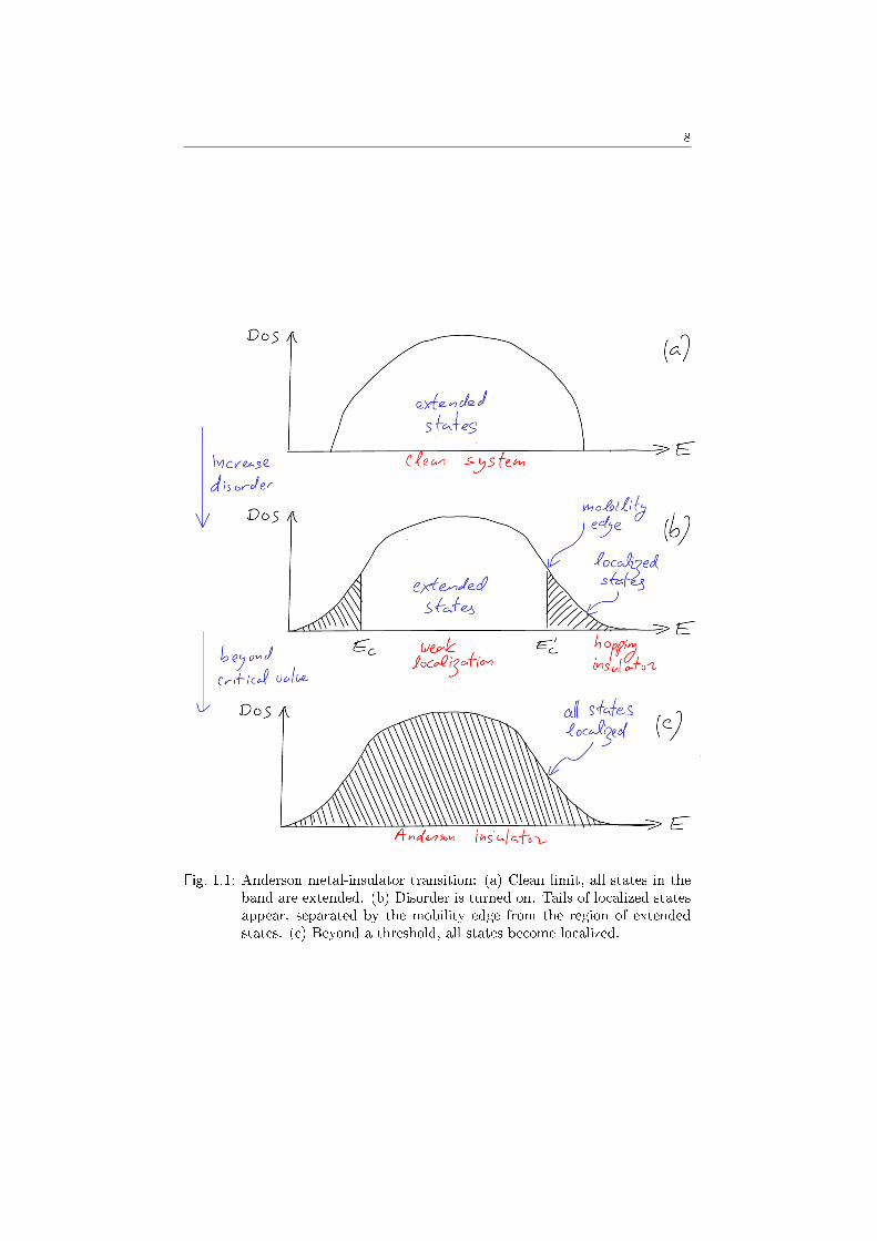
of the system d ≤ 2, then all eigenstates are localized (no matter how weak thedisorder is). For d = 3:

• Density of states forms tails of the band consisting of localized states

• Interior of the band corresponds to extended states

• Critical energies Ec, E′c separating localized from extended states are

called the mobility edges

Implications for transport:

• Only extended states contribute to transport/conductivity signicantly

7

• Position of mobility edge depends on the magnitude of disorder

• At critical magnitute of disorder: metal-insulator phase transition, i.e. allstates become localized (Anderson transition).

Current transport is by electrons with energy E ' EF . For EF < Ec (withinthe hopping regime):

• Current transport by localized electrons, electrons tunnel/hop from onelocalized state to the other

• Tunneling probability between localized wavefunctions α→ β: p(rαβ , Eβ , Eα) ∝e−αrαβe−(Eβ−Eα)/kBT , leading to Mott's law for conductivity: σ(T ) ∝e−(T0/T )1/4 (but at T → 0 the system is insulating).

For EF > Ec: Fermi-energy within region of extended states: metallic regime

• Disorder leads to positive interference of certain terms in perturbationexpansion of conductivity: enhanced backscattering (weak localization)leads to reduced conductivity.

• Externally applied magnetic eld destroys positive interference and weaklocalization (negative magnetoresistance, i.e. the decrease of resistancewith magnetic eld).

Dirac materials: weak anti-localisation

• Backscattering is forbidden due to a Berry phase eect in k-space (leadingin the presence of magnetic eld to positive magnetoresistance, i.e. theincrease of resistance with magnetic eld).

8

Fig. 1.1: Anderson metal-insulator transition: (a) Clean limit, all states in theband are extended. (b) Disorder is turned on. Tails of localized statesappear, separated by the mobility edge from the region of extendedstates. (c) Beyond a threshold, all states become localized.