Lecture 7 Time-dependent Covariates in Cox Regressionmath.ucsd.edu/~rxu/math284/slect7.pdf ·...

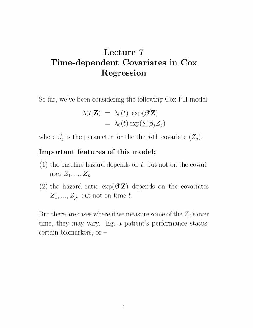
Lecture 7Time-dependent Covariates in Cox

Regression

So far, we’ve been considering the following Cox PH model:

λ(t|Z) = λ0(t) exp(β′Z)

= λ0(t) exp(∑βjZj)

where βj is the parameter for the the j-th covariate (Zj).

Important features of this model:

(1) the baseline hazard depends on t, but not on the covari-

ates Z1, ..., Zp

(2) the hazard ratio exp(β′Z) depends on the covariates

Z1, ..., Zp, but not on time t.

But there are cases where if we measure some of the Zj’s over

time, they may vary. Eg. a patient’s performance status,

certain biomarkers, or –

1

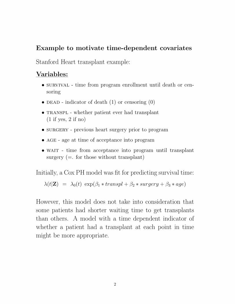
Example to motivate time-dependent covariates

Stanford Heart transplant example:

Variables:

• survival - time from program enrollment until death or cen-soring

• dead - indicator of death (1) or censoring (0)

• transpl - whether patient ever had transplant(1 if yes, 2 if no)

• surgery - previous heart surgery prior to program

• age - age at time of acceptance into program

• wait - time from acceptance into program until transplantsurgery (=. for those without transplant)

Initially, a Cox PH model was fit for predicting survival time:

λ(t|Z) = λ0(t) exp(β1 ∗ transpl + β2 ∗ surgery + β3 ∗ age)

However, this model does not take into consideration that

some patients had shorter waiting time to get transplants

than others. A model with a time dependent indicator of

whether a patient had a transplant at each point in time

might be more appropriate.

2

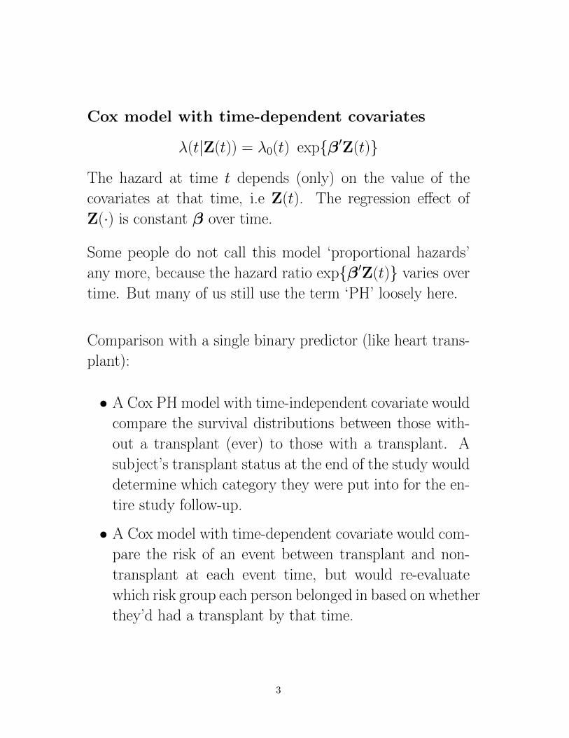
Cox model with time-dependent covariates

λ(t|Z(t)) = λ0(t) exp{β′Z(t)}

The hazard at time t depends (only) on the value of the

covariates at that time, i.e Z(t). The regression effect of

Z(·) is constant β over time.

Some people do not call this model ‘proportional hazards’

any more, because the hazard ratio exp{β′Z(t)} varies over

time. But many of us still use the term ‘PH’ loosely here.

Comparison with a single binary predictor (like heart trans-

plant):

• A Cox PH model with time-independent covariate would

compare the survival distributions between those with-

out a transplant (ever) to those with a transplant. A

subject’s transplant status at the end of the study would

determine which category they were put into for the en-

tire study follow-up.

• A Cox model with time-dependent covariate would com-

pare the risk of an event between transplant and non-

transplant at each event time, but would re-evaluate

which risk group each person belonged in based on whether

they’d had a transplant by that time.

3

Inference:

We still use the partial likelihood to estimate β

L(β) =n∏i=1

exp{β′Zi(Xi)}∑j∈R(Xi) exp{β′Zj(Xi)}

δi

Note that each term in the partial likelihood is still the con-

ditional probability of choosing individual i to fail from the

risk set, given the risk set at time Xi and given that one

failure is to occur.

Inference then proceeds similarly to the Cox model with

time-independent covariates. The only difference is that the

values of Z now changes at each risk set.

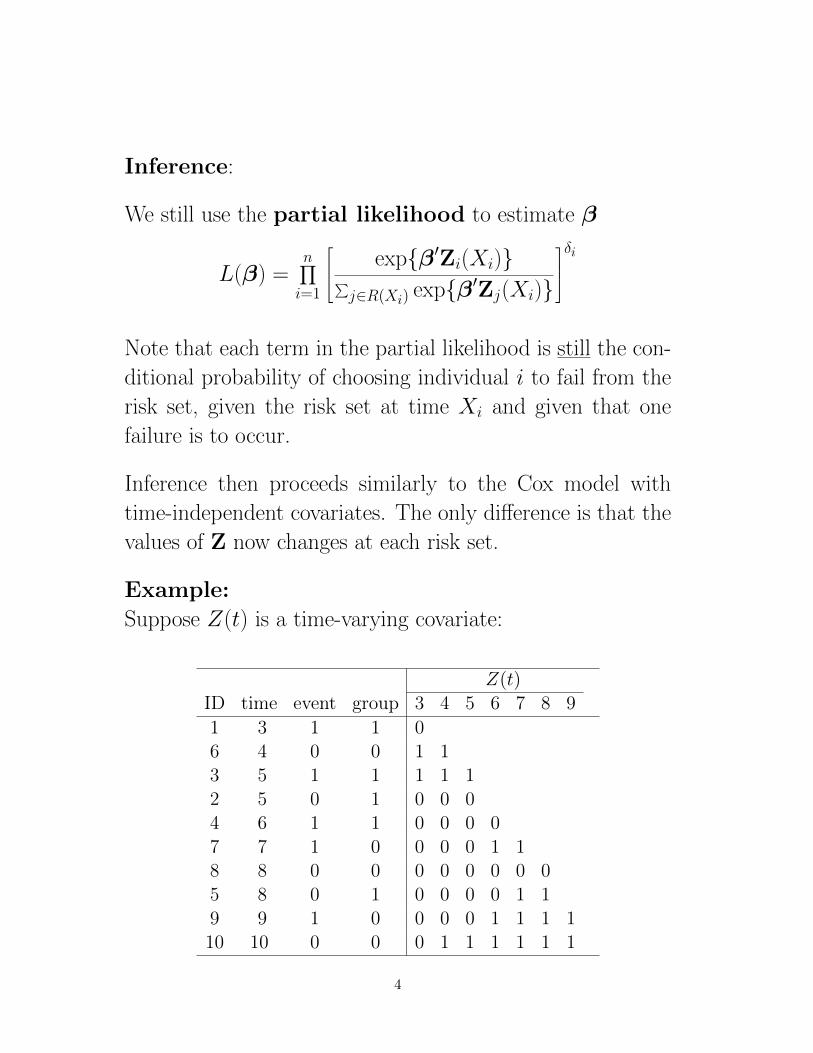
Example:

Suppose Z(t) is a time-varying covariate:

Z(t)ID time event group 3 4 5 6 7 8 9

1 3 1 1 06 4 0 0 1 13 5 1 1 1 1 12 5 0 1 0 0 04 6 1 1 0 0 0 07 7 1 0 0 0 0 1 18 8 0 0 0 0 0 0 0 05 8 0 1 0 0 0 0 1 19 9 1 0 0 0 0 1 1 1 110 10 0 0 0 1 1 1 1 1 1

4

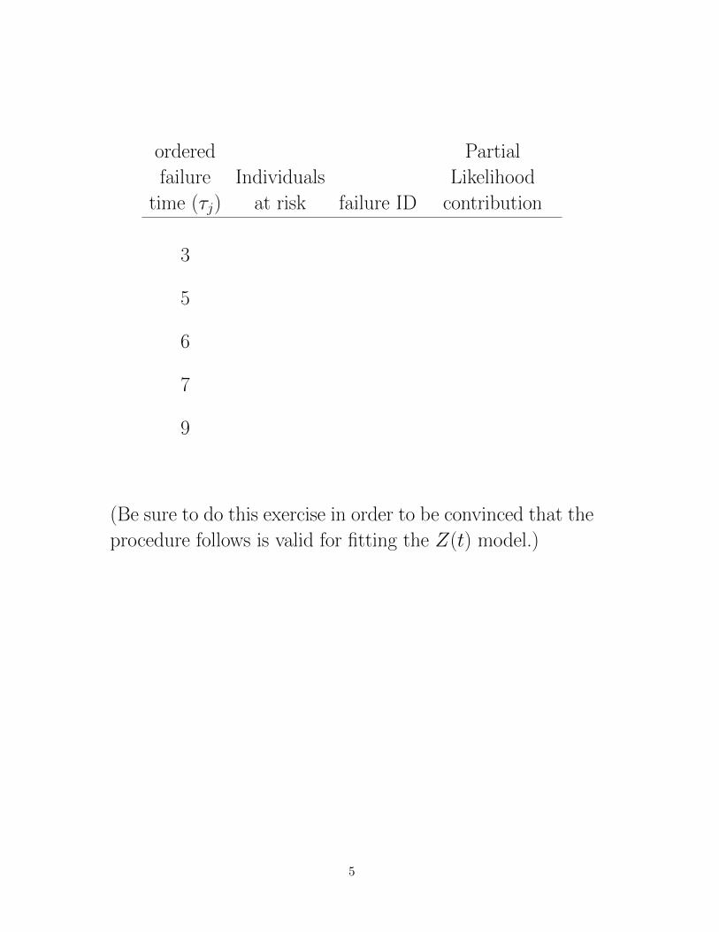
ordered Partial

failure Individuals Likelihood

time (τj) at risk failure ID contribution

3

5

6

7

9

(Be sure to do this exercise in order to be convinced that the

procedure follows is valid for fitting the Z(t) model.)

5

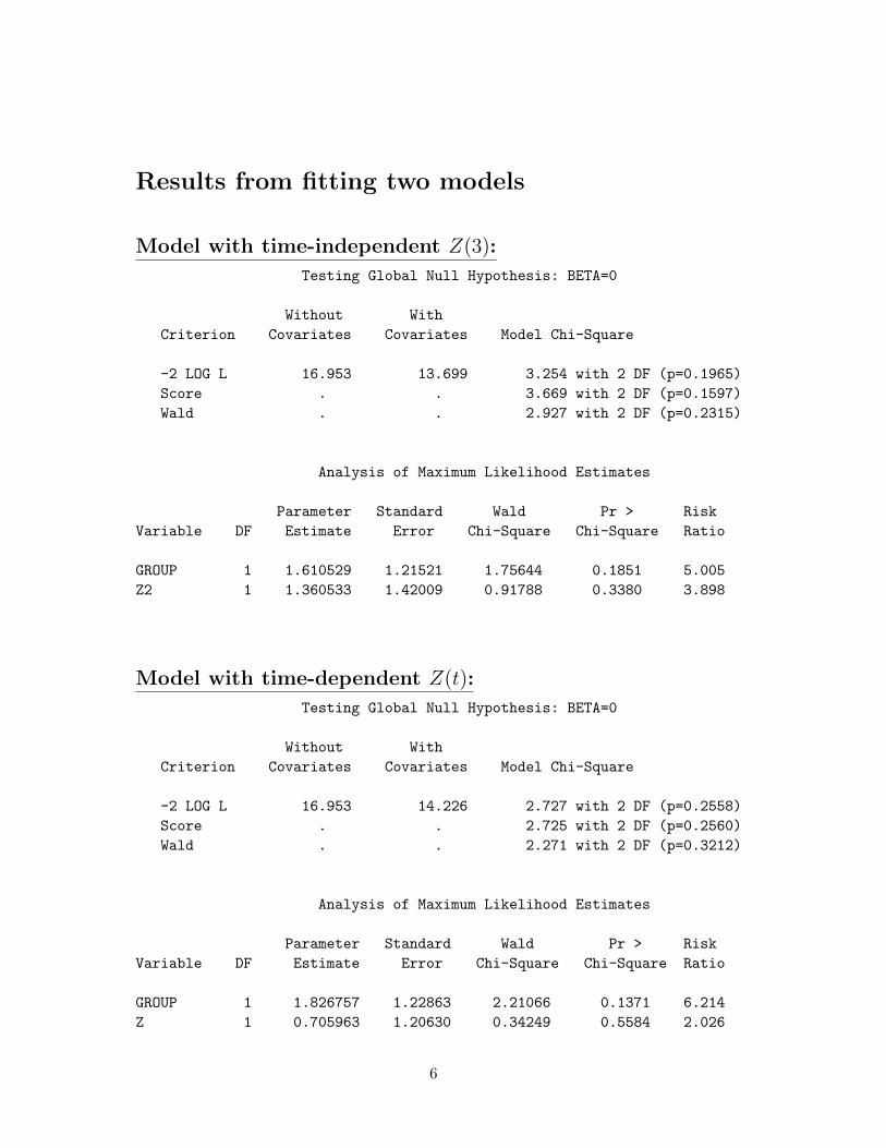
Results from fitting two models

Model with time-independent Z(3):

Testing Global Null Hypothesis: BETA=0

Without With

Criterion Covariates Covariates Model Chi-Square

-2 LOG L 16.953 13.699 3.254 with 2 DF (p=0.1965)

Score . . 3.669 with 2 DF (p=0.1597)

Wald . . 2.927 with 2 DF (p=0.2315)

Analysis of Maximum Likelihood Estimates

Parameter Standard Wald Pr > Risk

Variable DF Estimate Error Chi-Square Chi-Square Ratio

GROUP 1 1.610529 1.21521 1.75644 0.1851 5.005

Z2 1 1.360533 1.42009 0.91788 0.3380 3.898

Model with time-dependent Z(t):


Without With


-2 LOG L 16.953 14.226 2.727 with 2 DF (p=0.2558)

Score . . 2.725 with 2 DF (p=0.2560)

Wald . . 2.271 with 2 DF (p=0.3212)




GROUP 1 1.826757 1.22863 2.21066 0.1371 6.214

Z 1 0.705963 1.20630 0.34249 0.5584 2.026

6

Time-varying covariates in R (and most software)

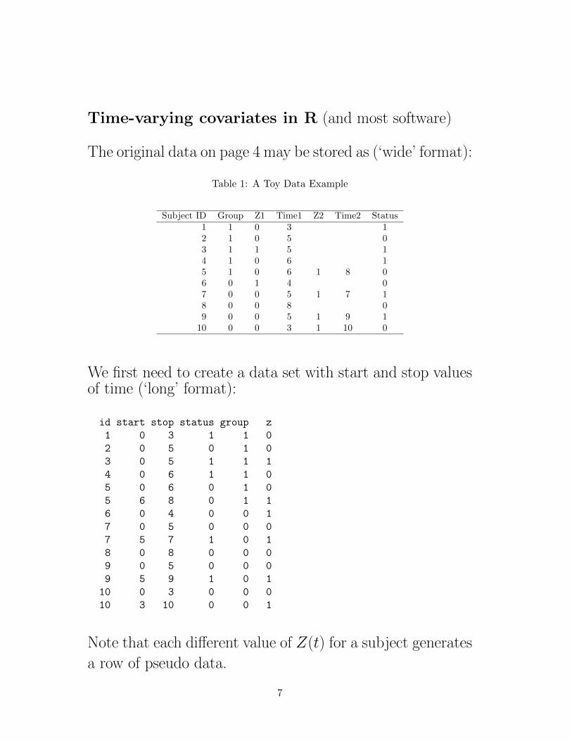
The original data on page 4 may be stored as (‘wide’ format):

Table 1: A Toy Data Example

Subject ID Group Z1 Time1 Z2 Time2 Status1 1 0 3 12 1 0 5 03 1 1 5 14 1 0 6 15 1 0 6 1 8 06 0 1 4 07 0 0 5 1 7 18 0 0 8 09 0 0 5 1 9 1

10 0 0 3 1 10 0

We first need to create a data set with start and stop valuesof time (‘long’ format):

id start stop status group z

1 0 3 1 1 0

2 0 5 0 1 0

3 0 5 1 1 1

4 0 6 1 1 0

5 0 6 0 1 0

5 6 8 0 1 1

6 0 4 0 0 1

7 0 5 0 0 0

7 5 7 1 0 1

8 0 8 0 0 0

9 0 5 0 0 0

9 5 9 1 0 1

10 0 3 0 0 0

10 3 10 0 0 1

Note that each different value of Z(t) for a subject generates

a row of pseudo data.

7

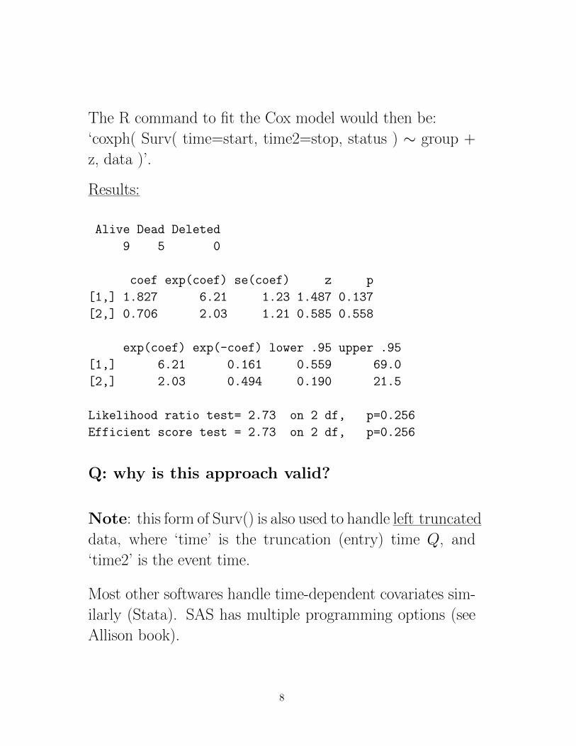
The R command to fit the Cox model would then be:

‘coxph( Surv( time=start, time2=stop, status ) ∼ group +

z, data )’.

Results:

Alive Dead Deleted

9 5 0

coef exp(coef) se(coef) z p

[1,] 1.827 6.21 1.23 1.487 0.137

[2,] 0.706 2.03 1.21 0.585 0.558

exp(coef) exp(-coef) lower .95 upper .95

[1,] 6.21 0.161 0.559 69.0

[2,] 2.03 0.494 0.190 21.5

Likelihood ratio test= 2.73 on 2 df, p=0.256

Efficient score test = 2.73 on 2 df, p=0.256

Q: why is this approach valid?

Note: this form of Surv() is also used to handle left truncated

data, where ‘time’ is the truncation (entry) time Q, and

‘time2’ is the event time.

Most other softwares handle time-dependent covariates sim-

ilarly (Stata). SAS has multiple programming options (see

Allison book).

8

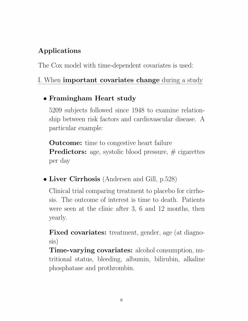
Applications

The Cox model with time-dependent covariates is used:

I. When important covariates change during a study

• Framingham Heart study

5209 subjects followed since 1948 to examine relation-

ship between risk factors and cardiovascular disease. A

particular example:

Outcome: time to congestive heart failure

Predictors: age, systolic blood pressure, # cigarettes

per day

• Liver Cirrhosis (Andersen and Gill, p.528)

Clinical trial comparing treatment to placebo for cirrho-

sis. The outcome of interest is time to death. Patients

were seen at the clinic after 3, 6 and 12 months, then

yearly.

Fixed covariates: treatment, gender, age (at diagno-

sis)

Time-varying covariates: alcohol consumption, nu-

tritional status, bleeding, albumin, bilirubin, alkaline

phosphatase and prothrombin.

9

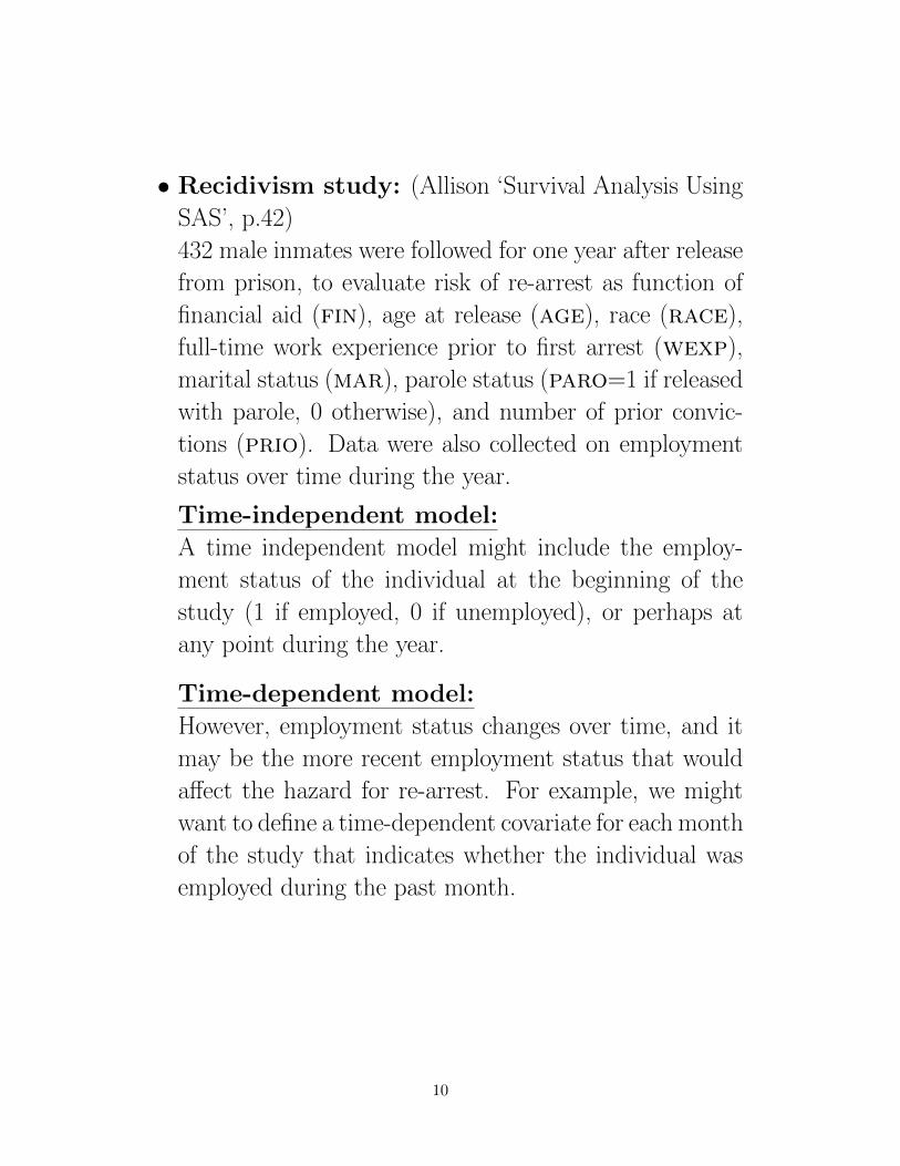
• Recidivism study: (Allison ‘Survival Analysis Using

SAS’, p.42)

432 male inmates were followed for one year after release

from prison, to evaluate risk of re-arrest as function of

financial aid (fin), age at release (age), race (race),

full-time work experience prior to first arrest (wexp),

marital status (mar), parole status (paro=1 if released

with parole, 0 otherwise), and number of prior convic-

tions (prio). Data were also collected on employment

status over time during the year.

Time-independent model:

A time independent model might include the employ-

ment status of the individual at the beginning of the

study (1 if employed, 0 if unemployed), or perhaps at

any point during the year.

Time-dependent model:

However, employment status changes over time, and it

may be the more recent employment status that would

affect the hazard for re-arrest. For example, we might

want to define a time-dependent covariate for each month

of the study that indicates whether the individual was

employed during the past month.

10

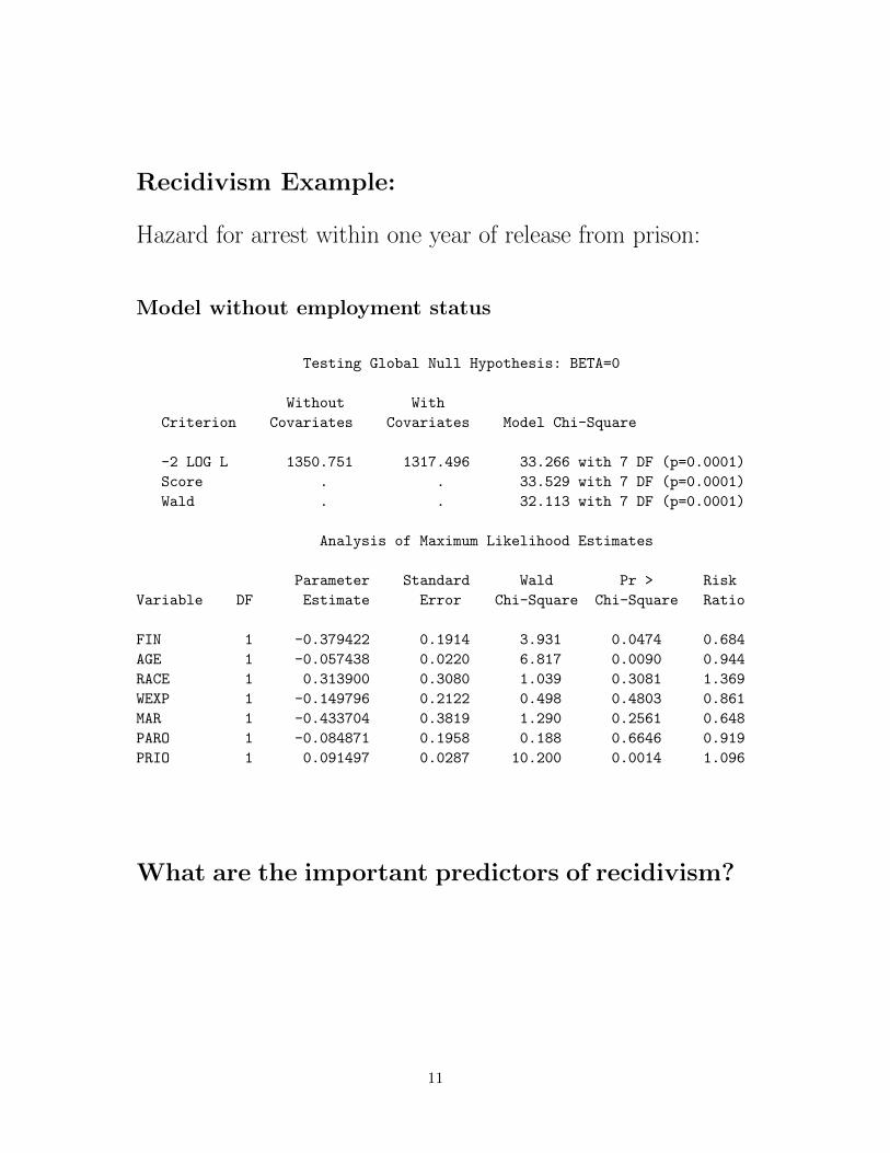
Recidivism Example:

Hazard for arrest within one year of release from prison:

Model without employment status


Without With


-2 LOG L 1350.751 1317.496 33.266 with 7 DF (p=0.0001)

Score . . 33.529 with 7 DF (p=0.0001)

Wald . . 32.113 with 7 DF (p=0.0001)




FIN 1 -0.379422 0.1914 3.931 0.0474 0.684

AGE 1 -0.057438 0.0220 6.817 0.0090 0.944

RACE 1 0.313900 0.3080 1.039 0.3081 1.369

WEXP 1 -0.149796 0.2122 0.498 0.4803 0.861

MAR 1 -0.433704 0.3819 1.290 0.2561 0.648

PARO 1 -0.084871 0.1958 0.188 0.6646 0.919

PRIO 1 0.091497 0.0287 10.200 0.0014 1.096

What are the important predictors of recidivism?

11

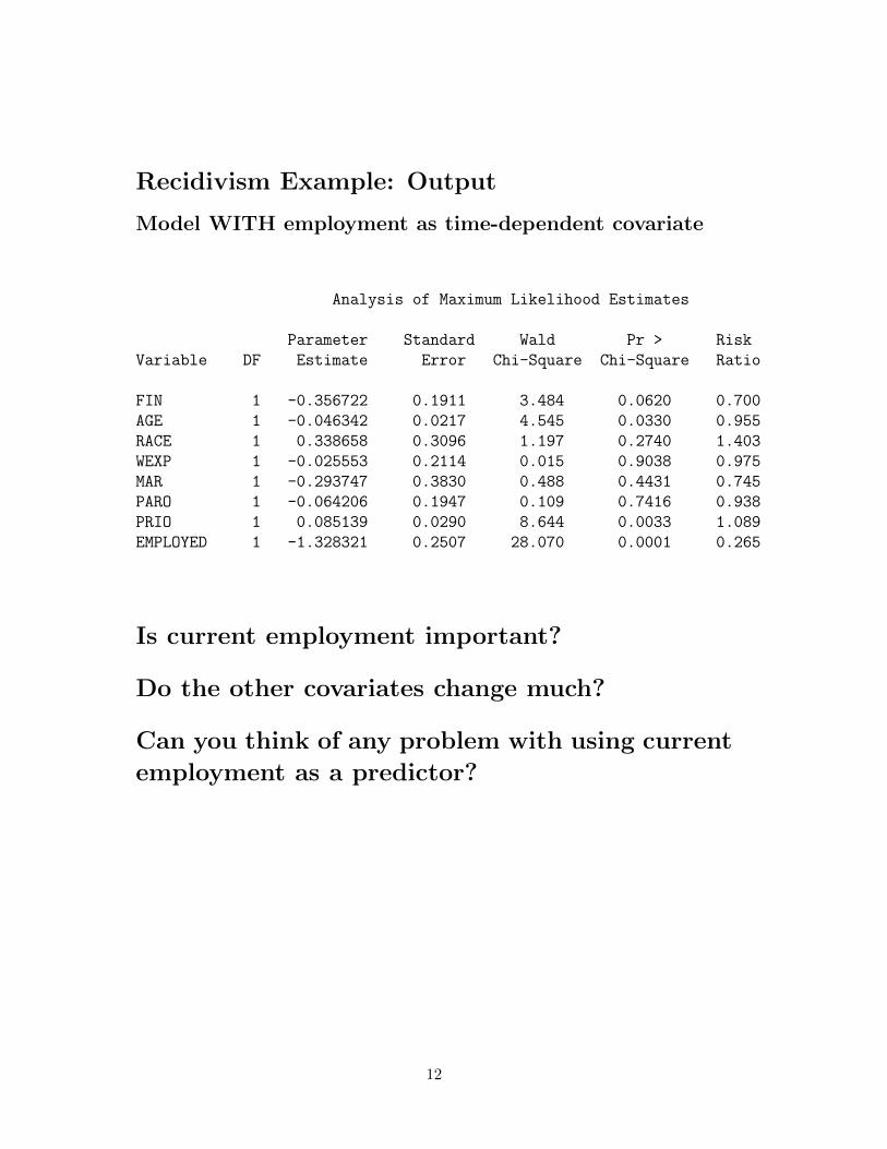
Recidivism Example: Output

Model WITH employment as time-dependent covariate




FIN 1 -0.356722 0.1911 3.484 0.0620 0.700

AGE 1 -0.046342 0.0217 4.545 0.0330 0.955

RACE 1 0.338658 0.3096 1.197 0.2740 1.403

WEXP 1 -0.025553 0.2114 0.015 0.9038 0.975

MAR 1 -0.293747 0.3830 0.488 0.4431 0.745

PARO 1 -0.064206 0.1947 0.109 0.7416 0.938

PRIO 1 0.085139 0.0290 8.644 0.0033 1.089

EMPLOYED 1 -1.328321 0.2507 28.070 0.0001 0.265

Is current employment important?

Do the other covariates change much?

Can you think of any problem with using current

employment as a predictor?

12

Another option for assessing impact of employ-

ment

Allison suggests using the employment status of the past

week rather than the current week.

The coefficient for employed changes from -1.33

to -0.79, so the risk ratio is about 0.45 instead of

0.27. It is still highly significant with χ2 = 13.1.

Does this model improve the causal interpretation?

Other options for time-dependent covariates:

• multiple lags of employment status (week-1, week-2, etc.)

• cumulative employment experience (proportion of weeks

worked)

13

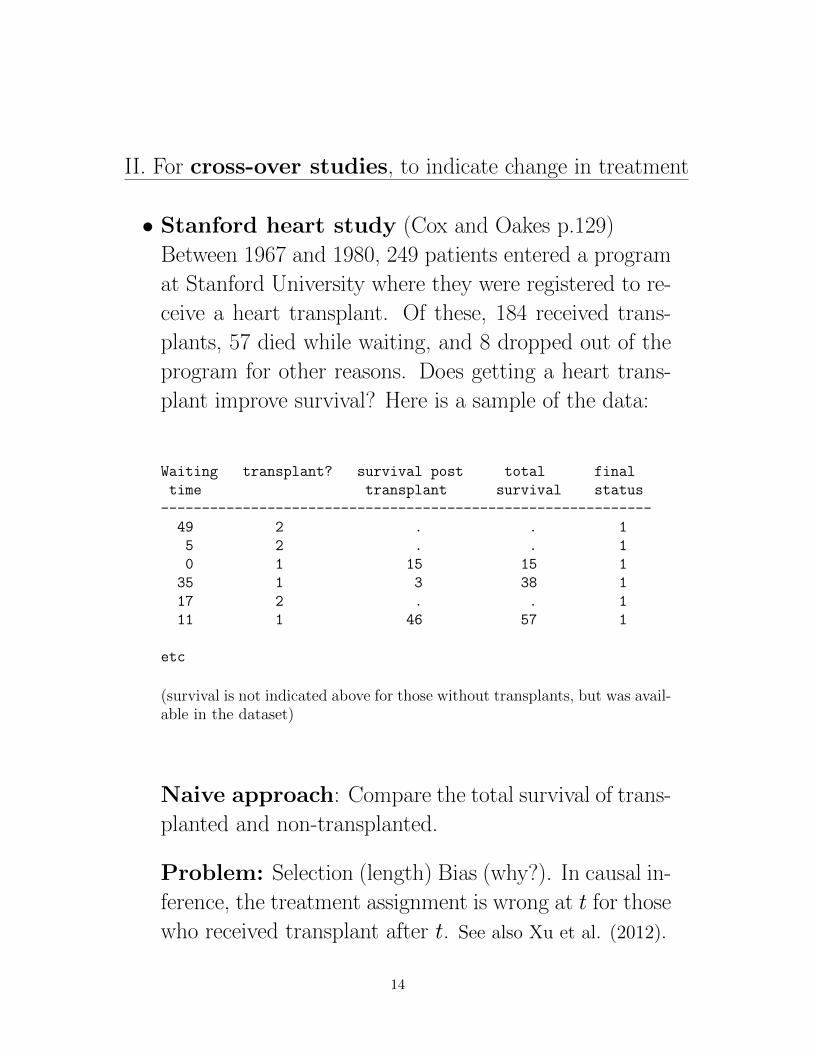
II. For cross-over studies, to indicate change in treatment

• Stanford heart study (Cox and Oakes p.129)

Between 1967 and 1980, 249 patients entered a program

at Stanford University where they were registered to re-

ceive a heart transplant. Of these, 184 received trans-

plants, 57 died while waiting, and 8 dropped out of the

program for other reasons. Does getting a heart trans-

plant improve survival? Here is a sample of the data:

Waiting transplant? survival post total final

time transplant survival status

------------------------------------------------------------

49 2 . . 1

5 2 . . 1

0 1 15 15 1

35 1 3 38 1

17 2 . . 1

11 1 46 57 1

etc

(survival is not indicated above for those without transplants, but was avail-able in the dataset)

Naive approach: Compare the total survival of trans-

planted and non-transplanted.

Problem: Selection (length) Bias (why?). In causal in-

ference, the treatment assignment is wrong at t for those

who received transplant after t. See also Xu et al. (2012).

14

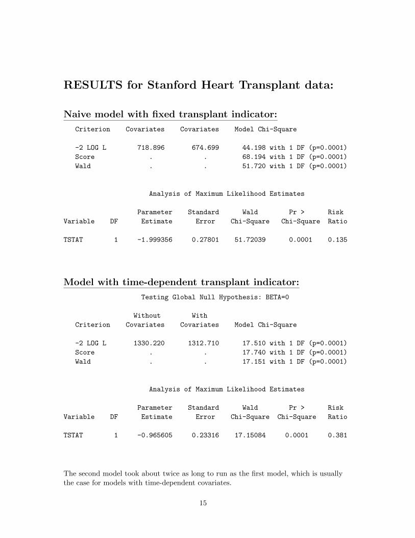
RESULTS for Stanford Heart Transplant data:

Naive model with fixed transplant indicator:


-2 LOG L 718.896 674.699 44.198 with 1 DF (p=0.0001)

Score . . 68.194 with 1 DF (p=0.0001)

Wald . . 51.720 with 1 DF (p=0.0001)




TSTAT 1 -1.999356 0.27801 51.72039 0.0001 0.135

Model with time-dependent transplant indicator:


Without With


-2 LOG L 1330.220 1312.710 17.510 with 1 DF (p=0.0001)

Score . . 17.740 with 1 DF (p=0.0001)

Wald . . 17.151 with 1 DF (p=0.0001)




TSTAT 1 -0.965605 0.23316 17.15084 0.0001 0.381

The second model took about twice as long to run as the first model, which is usuallythe case for models with time-dependent covariates.

15

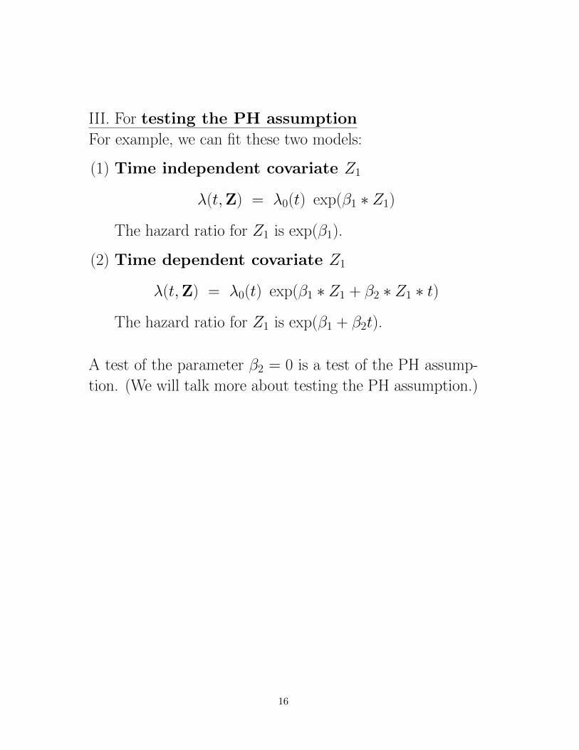
III. For testing the PH assumption

For example, we can fit these two models:

(1) Time independent covariate Z1

λ(t,Z) = λ0(t) exp(β1 ∗ Z1)

The hazard ratio for Z1 is exp(β1).

(2) Time dependent covariate Z1

λ(t,Z) = λ0(t) exp(β1 ∗ Z1 + β2 ∗ Z1 ∗ t)

The hazard ratio for Z1 is exp(β1 + β2t).

A test of the parameter β2 = 0 is a test of the PH assump-

tion. (We will talk more about testing the PH assumption.)

16

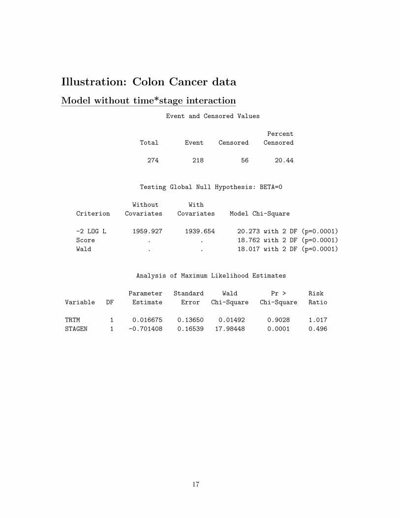
Illustration: Colon Cancer data

Model without time*stage interaction

Event and Censored Values

Percent

Total Event Censored Censored

274 218 56 20.44


Without With


-2 LOG L 1959.927 1939.654 20.273 with 2 DF (p=0.0001)

Score . . 18.762 with 2 DF (p=0.0001)

Wald . . 18.017 with 2 DF (p=0.0001)




TRTM 1 0.016675 0.13650 0.01492 0.9028 1.017

STAGEN 1 -0.701408 0.16539 17.98448 0.0001 0.496

17

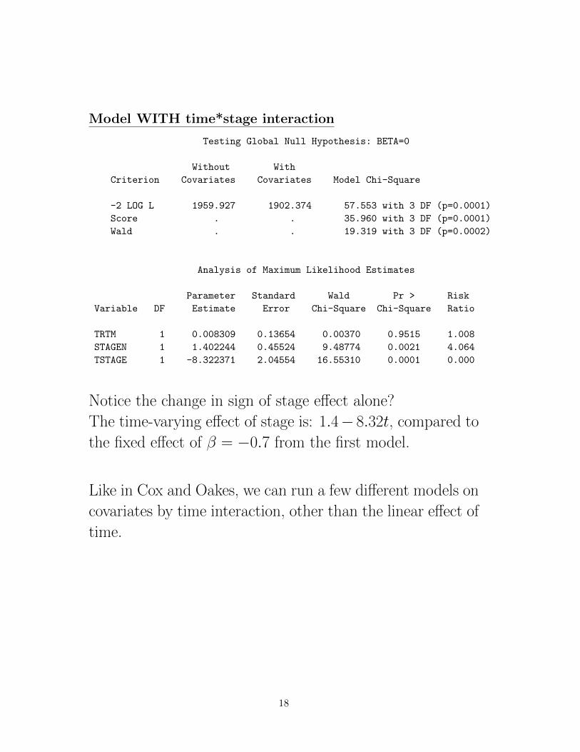
Model WITH time*stage interaction


Without With


-2 LOG L 1959.927 1902.374 57.553 with 3 DF (p=0.0001)

Score . . 35.960 with 3 DF (p=0.0001)

Wald . . 19.319 with 3 DF (p=0.0002)




TRTM 1 0.008309 0.13654 0.00370 0.9515 1.008

STAGEN 1 1.402244 0.45524 9.48774 0.0021 4.064

TSTAGE 1 -8.322371 2.04554 16.55310 0.0001 0.000

Notice the change in sign of stage effect alone?

The time-varying effect of stage is: 1.4− 8.32t, compared to

the fixed effect of β = −0.7 from the first model.

Like in Cox and Oakes, we can run a few different models on

covariates by time interaction, other than the linear effect of

time.

18

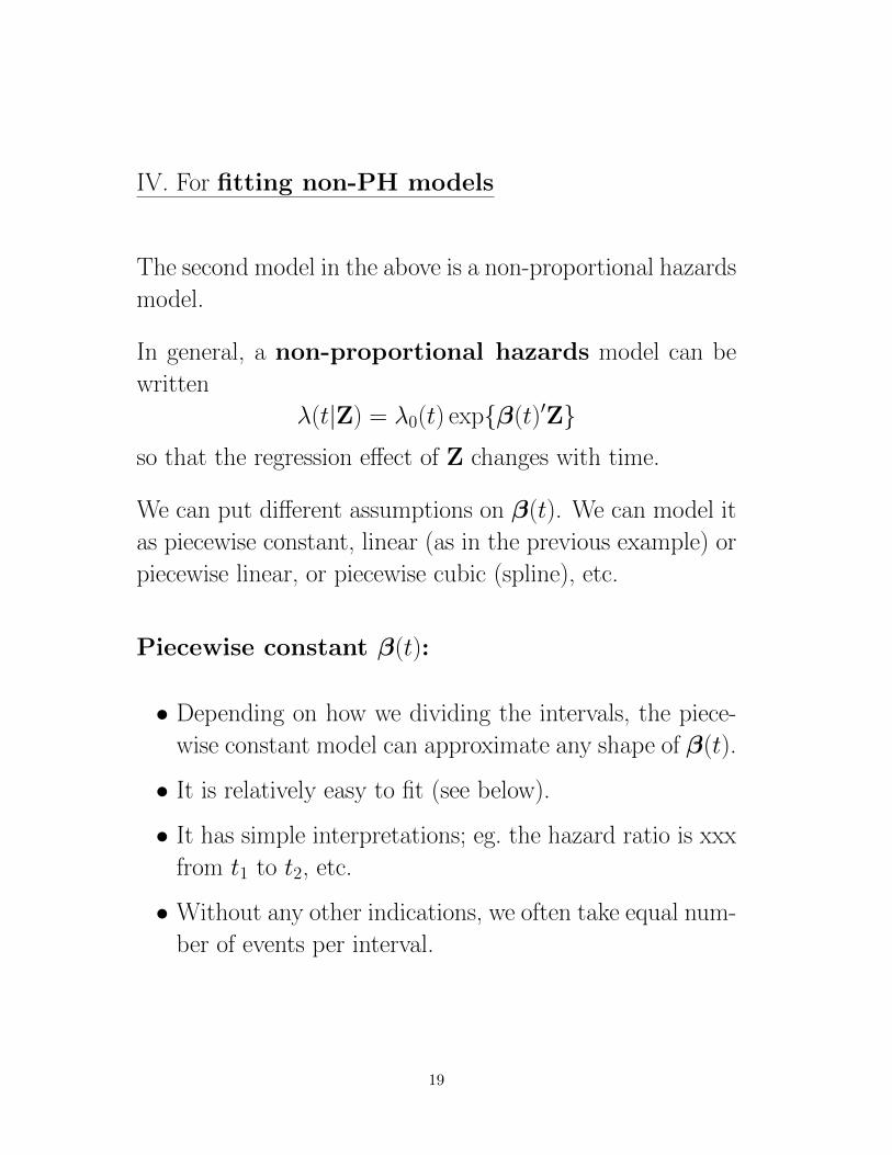
IV. For fitting non-PH models

The second model in the above is a non-proportional hazards

model.

In general, a non-proportional hazards model can be

written

λ(t|Z) = λ0(t) exp{β(t)′Z}so that the regression effect of Z changes with time.

We can put different assumptions on β(t). We can model it

as piecewise constant, linear (as in the previous example) or

piecewise linear, or piecewise cubic (spline), etc.

Piecewise constant β(t):

• Depending on how we dividing the intervals, the piece-

wise constant model can approximate any shape of β(t).

• It is relatively easy to fit (see below).

• It has simple interpretations; eg. the hazard ratio is xxx

from t1 to t2, etc.

• Without any other indications, we often take equal num-

ber of events per interval.

19

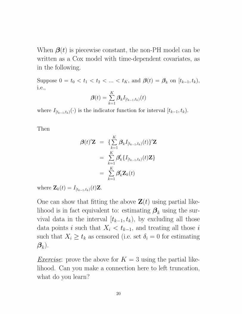
When β(t) is piecewise constant, the non-PH model can be

written as a Cox model with time-dependent covariates, as

in the following.

Suppose 0 = t0 < t1 < t2 < ... < tK , and β(t) = βk on [tk−1, tk),i.e.,

β(t) =K∑k=1

βkI[tk−1,tk)(t)

where I[tk−1,tk)(·) is the indicator function for interval [tk−1, tk).

Then

β(t)′Z = {K∑k=1

βkI[tk−1,tk)(t)}′Z

=K∑k=1

β′k{I[tk−1,tk)(t)Z}

=K∑k=1

β′kZk(t)

where Zk(t) = I[tk−1,tk)(t)Z.

One can show that fitting the above Z(t) using partial like-

lihood is in fact equivalent to: estimating βk using the sur-

vival data in the interval [tk−1, tk), by excluding all those

data points i such that Xi < tk−1, and treating all those i

such that Xi ≥ tk as censored (i.e. set δi = 0 for estimating

βk).

Exercise: prove the above for K = 3 using the partial like-

lihood. Can you make a connection here to left truncation,

what do you learn?

20

There are ways to search for an optimal change point of β(t);

see OQuigley and Pessione (1991).

There are also ways to find multiple change points using a

tree-based approach, following which a piecewise constant

β(t) can be fitted; see Xu and Adak (2002).

21

Some further notes

In practice, Z(t) may not be measured at each time point t.

What do we do?

• use the most recent value (assumes step function)

• interpolate

• impute based on some model for the ‘missing’ mechanism

Types of time-varying covariates:

• internal covariates:

variables that relate to the individuals, and can only be

measured when an individual is alive, e.g. white blood

cell count, CD4 count

• external covariates:

– variable which changes in a known way, e.g. age, dose

of drug

– variable that exists totally independently of all indi-

viduals, e.g. air temperature

These concepts are relavent particularly when predicting sur-

vival (estimating S(t|Z)). It is difficult to predict survival

based on internal covariates. Often survival prediction is

done only based on time-independent covariates.

22

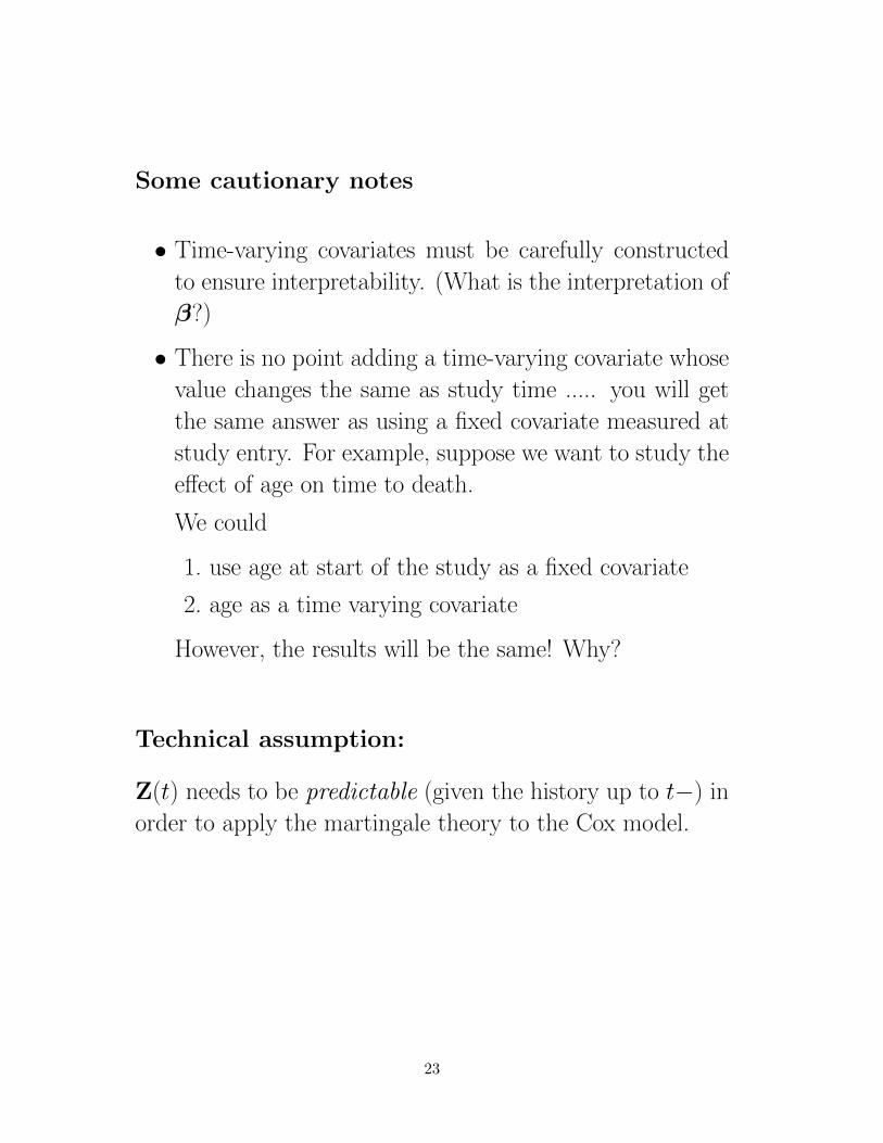
Some cautionary notes

• Time-varying covariates must be carefully constructed

to ensure interpretability. (What is the interpretation of

β?)

• There is no point adding a time-varying covariate whose

value changes the same as study time ..... you will get

the same answer as using a fixed covariate measured at

study entry. For example, suppose we want to study the

effect of age on time to death.

We could

1. use age at start of the study as a fixed covariate

2. age as a time varying covariate

However, the results will be the same! Why?

Technical assumption:

Z(t) needs to be predictable (given the history up to t−) in

order to apply the martingale theory to the Cox model.

23

Lecture 7 Time-dependent Covariates in Cox Regressionmath.ucsd.edu/~rxu/math284/slect7.pdf ·...

Documents

Transcript of Lecture 7 Time-dependent Covariates in Cox Regressionmath.ucsd.edu/~rxu/math284/slect7.pdf ·...