Lecture 21 Wave Propagation in Lossy Media and Poynting’s Theorem

5/13/2018 Lecture 21 Wave Propagation in Lossy Media and Poynting s Theorem - slidepdf.com

http://slidepdf.com/reader/full/lecture-21-wave-propagation-in-lossy-media-and-poyntings-theorem 1/18

EECS 117

Lecture 21: Wave Propagation in Lossy Media and

Poynting’s Theorem

Prof. Niknejad

University of California, Berkeley

Universit of California Berkele EECS 117 Lecture 21 – . 1/



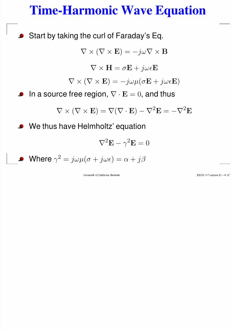
Time-Harmonic Wave Equation

Start by taking the curl of Faraday’s Eq.

∇× (∇× E) = − jω∇×B

∇×H = σE+ jωǫE

∇× (∇× E) = − jωµ(σE+ jωǫE)

In a source free region, ∇ · E = 0, and thus

∇× (∇× E) = ∇(∇ · E)−∇2E = −∇2

E

We thus have Helmholtz’ equation

∇2E− γ 2E = 0

Where γ 2 = jωµ(σ + jωǫ) = α + jβ




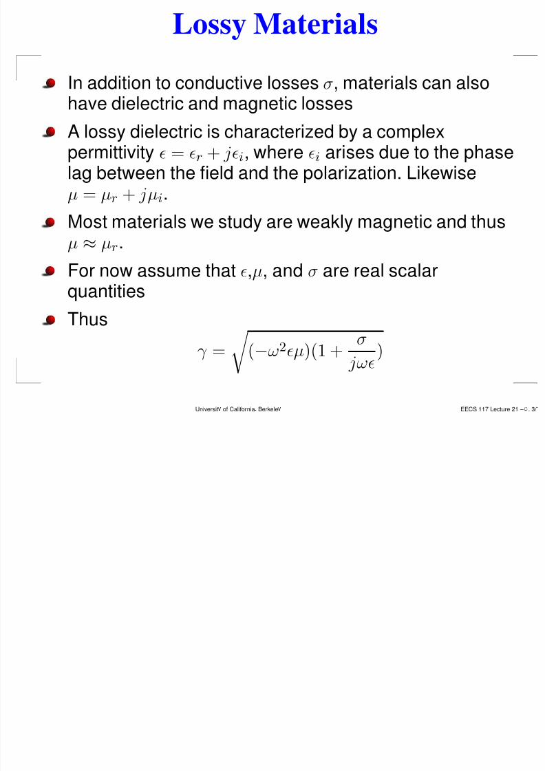
Lossy Materials

In addition to conductive losses σ, materials can alsohave dielectric and magnetic losses

A lossy dielectric is characterized by a complexpermittivity ǫ = ǫr + jǫi, where ǫi arises due to the phaselag between the field and the polarization. Likewiseµ = µr + jµi.

Most materials we study are weakly magnetic and thusµ ≈ µr.

For now assume that ǫ,µ, and σ are real scalar

quantities

Thus

γ = (−ω2ǫµ)(1 +σ

jωǫ)




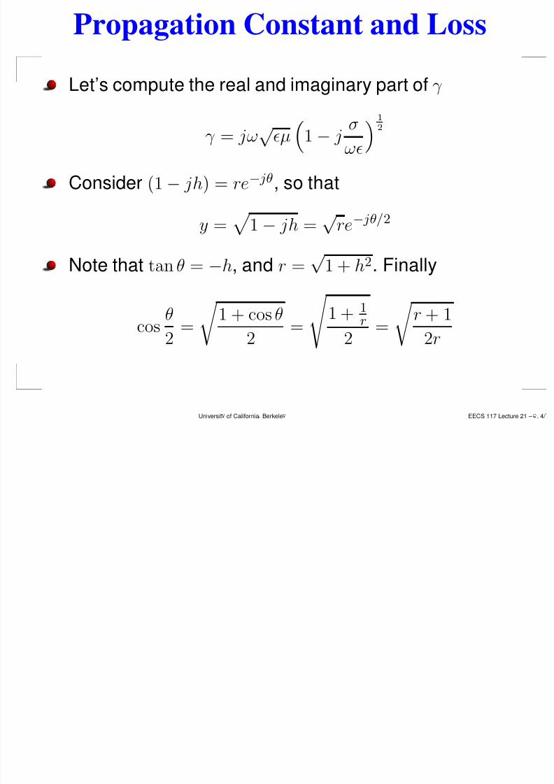
Propagation Constant and Loss

Let’s compute the real and imaginary part of γ

γ = jω√ǫµ1

− jσ

ωǫ

1

2

Consider (1− jh) = re− jθ, so that

y =

1− jh = √re− jθ/2

Note that tan θ = −h, and r =√

1 + h2. Finally

cosθ

2=

1 + cos θ

2=

1 + 1

r

2=

r + 1

2r




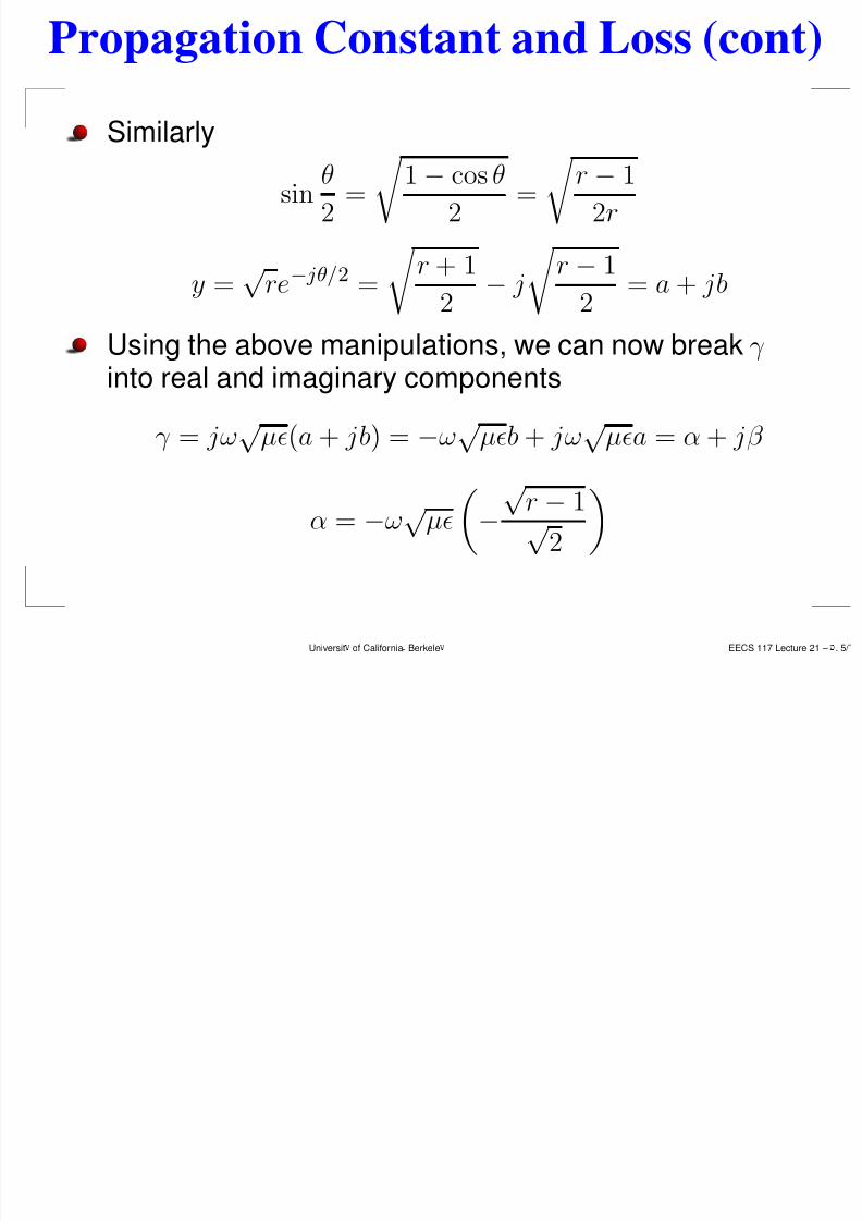
Propagation Constant and Loss (cont)

Similarly

sinθ

2=

1− cos θ

2=

r − 1

2r

y =√re− jθ/2 =

r + 1

2− j

r − 1

2= a + jb

Using the above manipulations, we can now break γ into real and imaginary components

γ = jω√µǫ(a + jb) =

−ω√µǫb + jω

√µǫa = α + jβ

α = −ω√µǫ

−√r − 1√

2




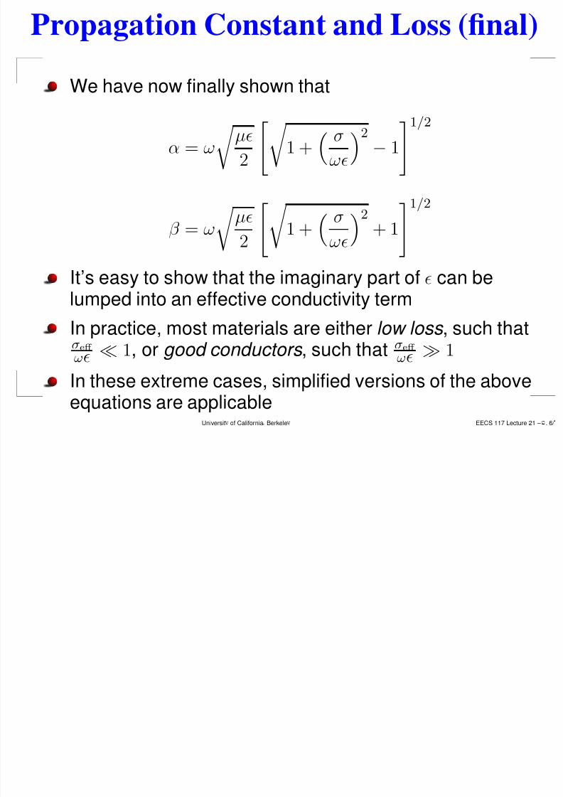
Propagation Constant and Loss (final)

We have now finally shown that

α = ω µǫ

2

1 + σ

ωǫ2 − 1

1/2

β = ω

µǫ2

1 +σωǫ2

+ 11/2

It’s easy to show that the imaginary part of ǫ can be

lumped into an effective conductivity termIn practice, most materials are either low loss , such thatσeff

ωǫ ≪ 1, or good conductors , such that σeff

ωǫ ≫ 1

In these extreme cases, simplified versions of the aboveequations are applicable




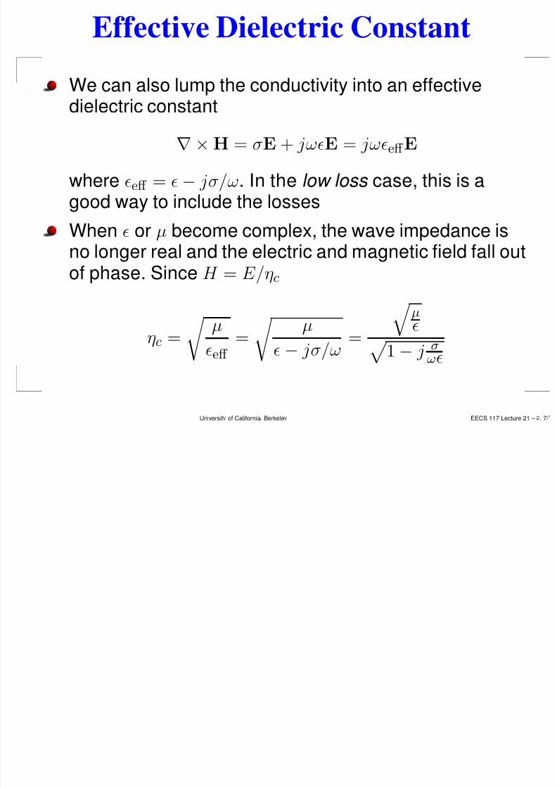
Effective Dielectric Constant

We can also lump the conductivity into an effectivedielectric constant

∇×H = σE + jωǫE = jωǫeff E

where ǫeff = ǫ− jσ/ω. In the low loss case, this is agood way to include the losses

When ǫ or µ become complex, the wave impedance isno longer real and the electric and magnetic field fall outof phase. Since H = E/ηc

ηc =

µ

ǫeff =

µ

ǫ

− jσ/ω

=

µǫ

1− j σωǫ




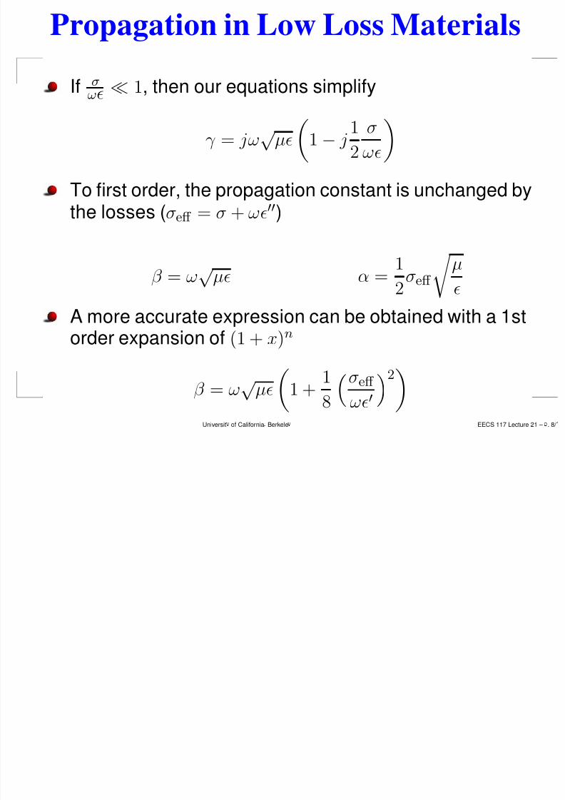
Propagation in Low Loss Materials

If σωǫ ≪ 1, then our equations simplify

γ = jω√µǫ1

− j

1

2

σ

ωǫ

To first order, the propagation constant is unchanged bythe losses (σeff = σ + ωǫ′′)

β = ω√µǫ α =

1

2σeff

µ

ǫ

A more accurate expression can be obtained with a 1storder expansion of (1 + x)n

β = ω√µǫ

1 + 18

σeff

ωǫ′

2




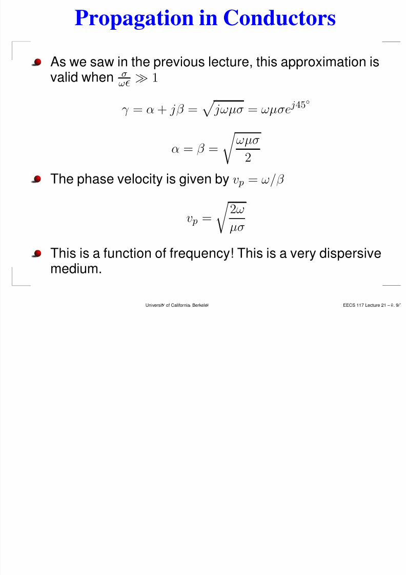
Propagation in Conductors

As we saw in the previous lecture, this approximation isvalid when σ

ωǫ ≫ 1

γ = α + jβ = jωµσ = ωµσe j

45◦

α = β = ωµσ2

The phase velocity is given by v p = ω/β

v p = 2ω

µσ

This is a function of frequency! This is a very dispersive

medium.




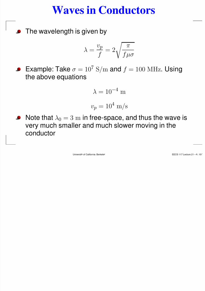
Waves in Conductors

The wavelength is given by

λ =v p

f = 2 π

fµσ

Example: Take σ = 107 S/m and f = 100 MHz. Usingthe above equations

λ = 10−4 m

v p = 10

4

m/sNote that λ0 = 3 m in free-space, and thus the wave isvery much smaller and much slower moving in theconductor




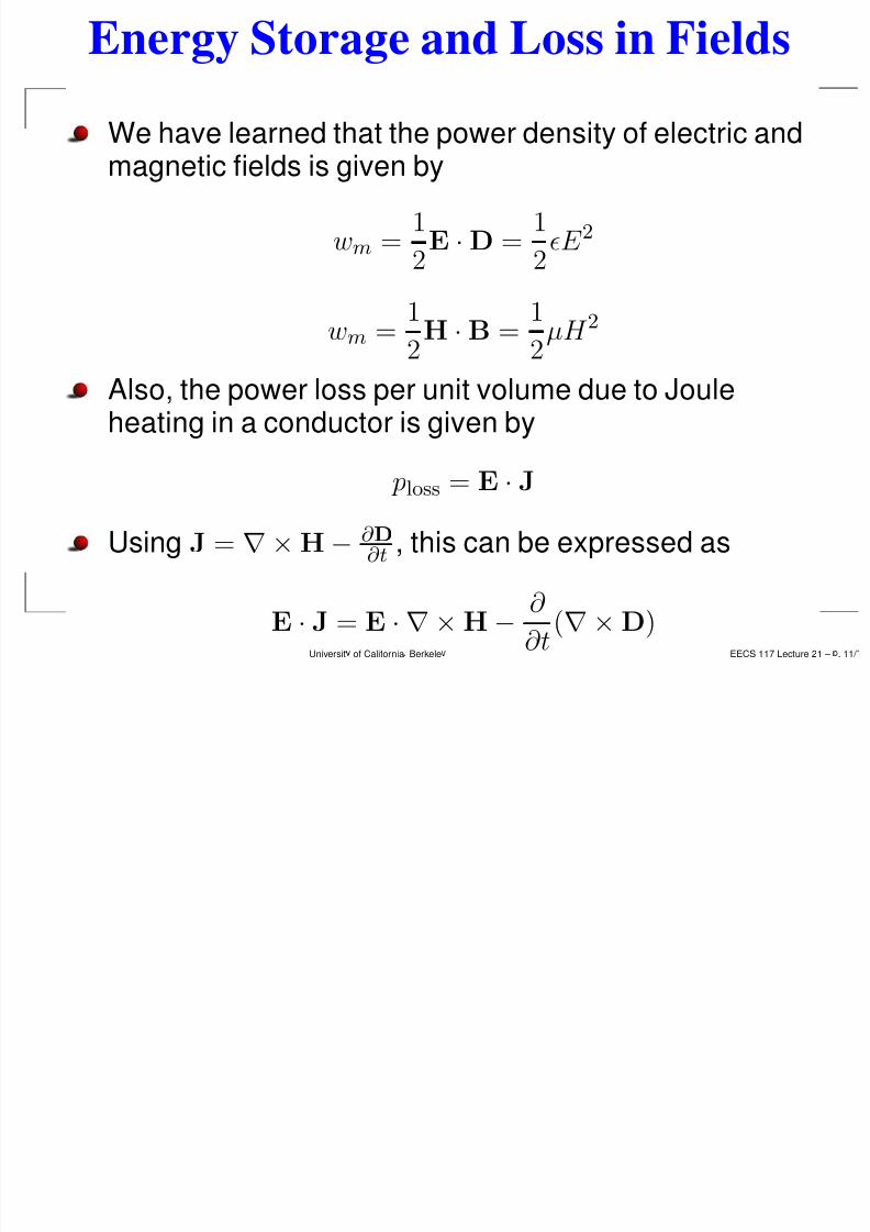
Energy Storage and Loss in Fields

We have learned that the power density of electric andmagnetic fields is given by

wm = 12E ·D = 1

2ǫE 2

wm =1

2H

·B =

1

2µH 2

Also, the power loss per unit volume due to Jouleheating in a conductor is given by

ploss = E · J

Using J = ∇×H− ∂ D∂t , this can be expressed as

E · J = E · ∇ ×H− ∂

∂t(∇×D)




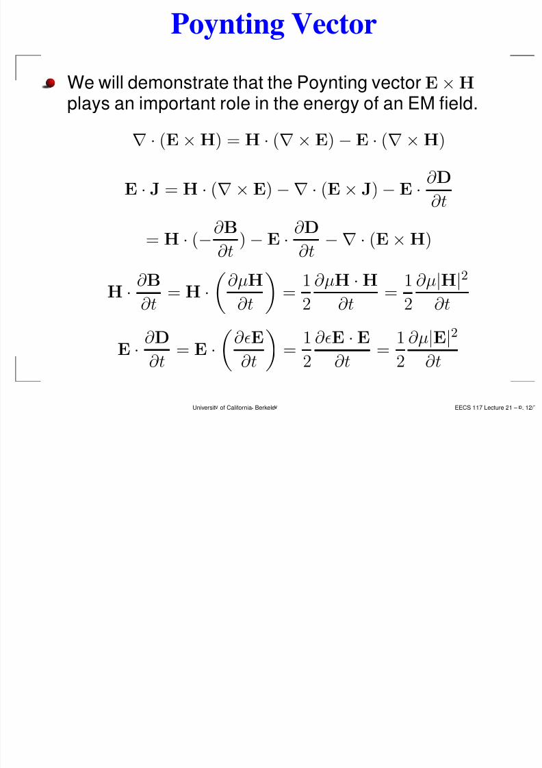
Poynting Vector

We will demonstrate that the Poynting vector E×Hplays an important role in the energy of an EM field.

∇ · (E×H) = H · (∇×E)−E · (∇×H)

E · J = H · (∇× E)−∇ · (E× J)− E · ∂ D∂t

= H · (−∂ B

∂t)− E · ∂ D

∂t−∇ · (E×H)

H · ∂ B

∂t = H · ∂µH

∂t

= 12 ∂µH

·H

∂t = 12 ∂µ|H

|2

∂t

E

·∂ D

∂t= E

·∂ǫE

∂t =

1

2

∂ǫE ·E∂t

=1

2

∂µ|E|2

∂t




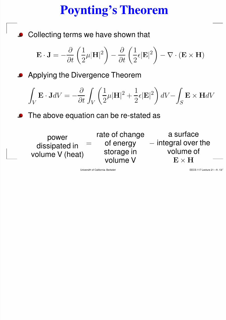
Poynting’s Theorem

Collecting terms we have shown that

E

·J =

−∂

∂t1

2µ|H

|2−

∂

∂t1

2ǫ|E

|2−∇ · (E

×H)

Applying the Divergence Theorem

V E · JdV = − ∂

∂t

V

12µ|H|2 + 1

2ǫ|E|2

dV −

S E×HdV

The above equation can be re-stated as

powerdissipated in

volume V (heat)

=rate of change

of energy

storage involume V

−

a surfaceintegral over the

volume ofE×H




Interpretation of the Poynting Vector

We now have a physical interpretation of the last term inthe above equation. By the conservation of energy, itmust be equal to the energy flow into or out of the

volumeWe may be so bold, then, to interpret the vectorS = E×H as the energy flow density of the field

While this seems reasonable, it’s important to note thatthe physical meaning is only attached to the integral ofS and not to discrete points in space


C C i i



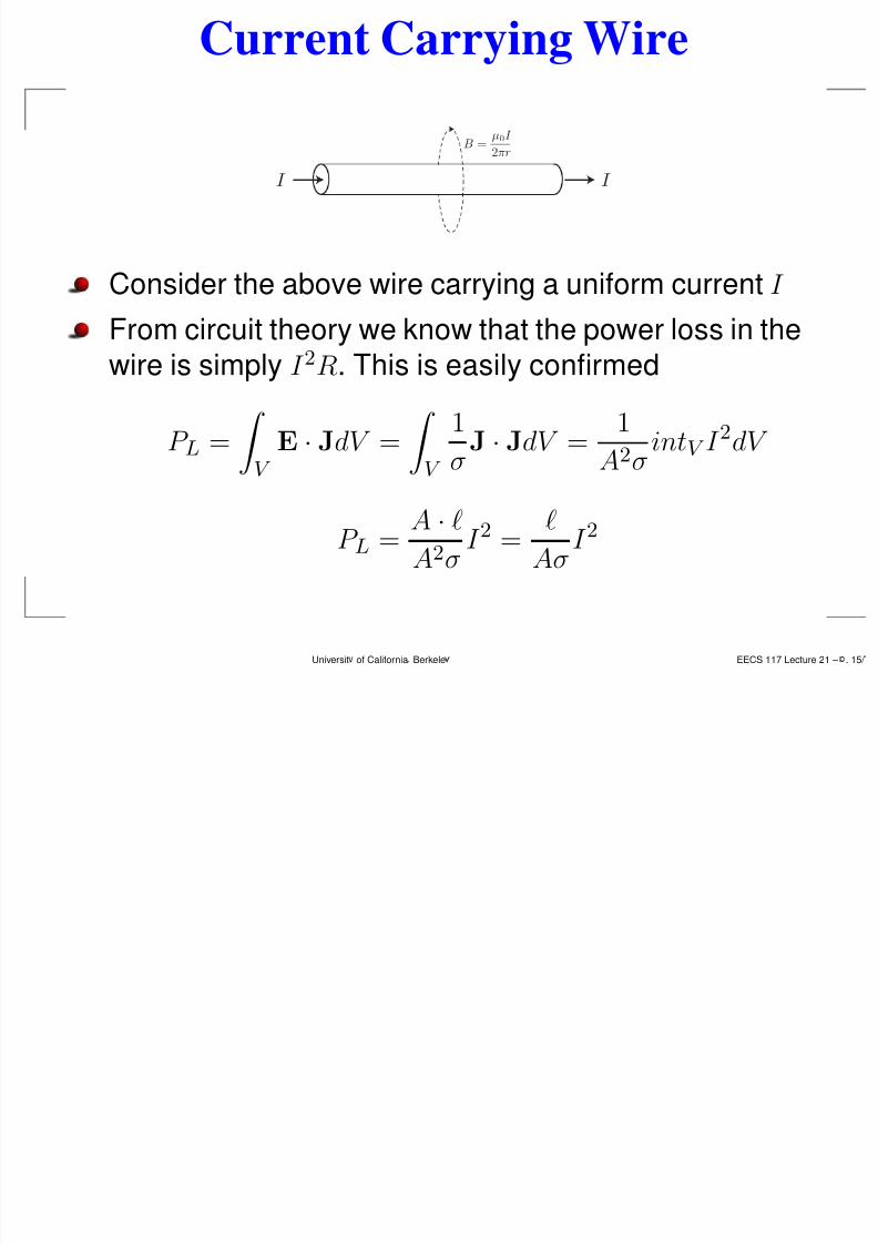
Current Carrying Wire

I I

B =µ0I

2πr

Consider the above wire carrying a uniform current I

From circuit theory we know that the power loss in the

wire is simply I 2R. This is easily confirmed

P L = V

E

·JdV =

V

1

σ

J

·JdV =

1

A2

σ

intV I 2dV

P L =A · ℓA2σ

I 2 =ℓ

AσI 2


E S d d Wi S i



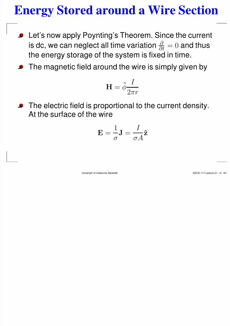
Energy Stored around a Wire Section

Let’s now apply Poynting’s Theorem. Since the current

is dc, we can neglect all time variation ∂ ∂t = 0 and thus

the energy storage of the system is fixed in time.

The magnetic field around the wire is simply given by

H = φI

2πr

The electric field is proportional to the current density.At the surface of the wire

E =1

σJ =

I

σAz




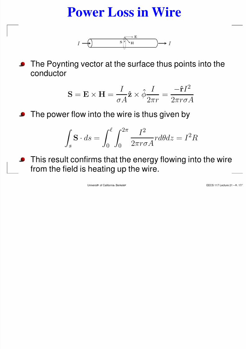
Power Loss in Wire

I I H

E

S

The Poynting vector at the surface thus points into theconductor

S = E

×H =

I

σAz

×φ

I

2πr=

−rI 22πrσA

The power flow into the wire is thus given by

sS · ds =

ℓ

0

2π

0

I 22πrσA

rdθdz = I 2R

This result confirms that the energy flowing into the wirefrom the field is heating up the wire.


S d Fi ld



Sources and Fields

This result is surprising because it hints that the signalin a wire is carried by the fields, and not by the charges.

In other words, if a signal propagates down a wire, the

information is carried by the fields, and the current flowis impressed upon the conductor from the fields.

We know that the sources of EM fields are charges and

currents. But we also know that if the configuration ofcharges changes, the fields “carry” this information


Lecture 21 Wave Propagation in Lossy Media and Poynting’s Theorem

Documents

Transcript of Lecture 21 Wave Propagation in Lossy Media and Poynting’s Theorem