Wave Propagation in Heterogeneous Media: Born and Rytov Approximations

Chris Sherman

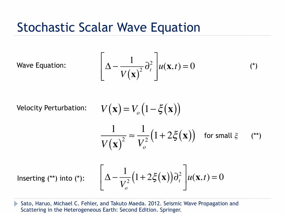
Stochastic Scalar Wave Equation

! " 1V x( )2

#t2

$

%&&

'

())u(x, t) = 0

V x( ) =Vo 1!! x( )( )

Wave Equation:

Velocity Perturbation:

1V x( )2

! 1Vo2 1+ 2! x( )( ) for small ξ (**)

(*)

Inserting (**) into (*): ! " 1Vo2 1+ 2! x( )( )#t2$

%&

'

()u(x, t) = 0

Sato, Haruo, Michael C. Fehler, and Takuto Maeda. 2012. Seismic Wave Propagation and Scattering in the Heterogeneous Earth : Second Edition. Springer.

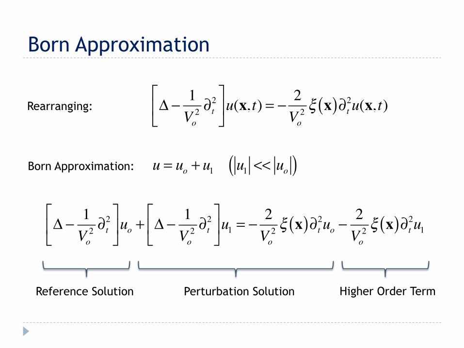
Born Approximation

Rearranging: ! " 1Vo2 #t

2$

%&

'

()u(x, t) = " 2

Vo2 ! x( )#t2u(x, t)

Born Approximation: u = uo + u1 u1 << uo( )

! " 1Vo2 #t

2$

%&

'

()uo + ! " 1

Vo2 #t

2$

%&

'

()u1 = " 2

Vo2 ! x( )#t2uo "

2Vo2 ! x( )#t2u1

Reference Solution Perturbation Solution Higher Order Term

Reference Solution

! " 1Vo2 #t

2$

%&

'

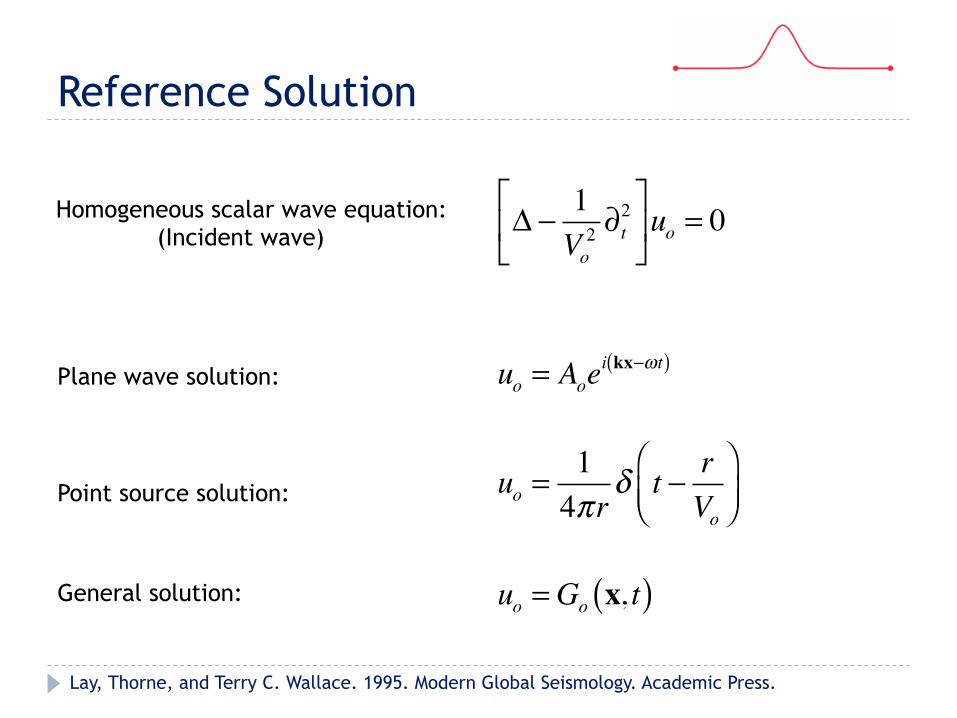
()uo = 0

Homogeneous scalar wave equation: (Incident wave)

Plane wave solution: uo = Aoei kx!!t( )

General solution: uo =Go x, t( )

Point source solution: uo =14!r

! t ! rVo

"#$

%&'

Lay, Thorne, and Terry C. Wallace. 1995. Modern Global Seismology. Academic Press.

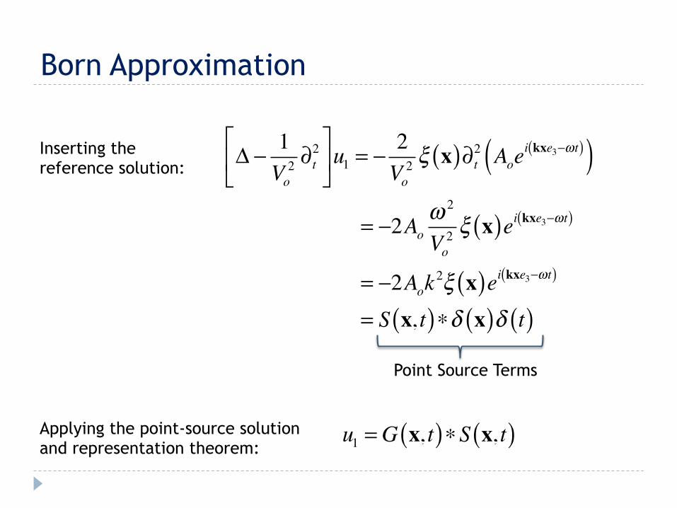
Born Approximation

! " 1Vo2 #t

2$

%&

'

()u1 = " 2

Vo2 ! x( )#t2 Aoe

i kxe3"!t( )( )= "2Ao

! 2

Vo2 ! x( )ei kxe3"!t( )

= "2Aok2! x( )ei kxe3"!t( )

= S x, t( )*! x( )! t( )

Inserting the reference solution:

Point Source Terms

Applying the point-source solution and representation theorem:

u1 =G x, t( )!S x, t( )

Born Approximation

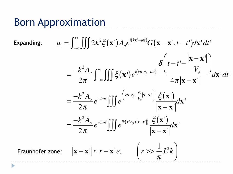
Expanding: u1 = 2k2! x '( )Aoei kx '!!t( )G x ! x ', t ! t '( )"""!#

#

" dx 'dt '

= !k2Ao2!

" x '( )ei kx 'e3!!t( )! t ! t '! x ! x '

Vo

$%&

'()

4! x ! x '"""!#

#

" dx 'dt '

= !k2Ao2!

e!i"t ei kx 'e3+

!Vox!x '

$%&

'() ! x '( )x ! x '""" dx '

= !k2Ao2!

e!i"t eik x 'e3+ x!x '( ) ! x '( )x ! x '""" dx '

Fraunhofer zone: x ! x ' " r ! x 'er r >> 1!L2k#

$%&'(

Born Approximation

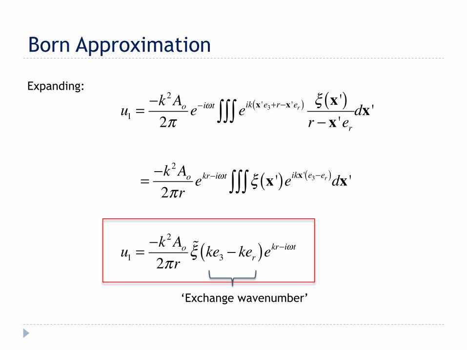
Expanding:

u1 =!k2Ao2!

e!i"t eik x 'e3+r!x 'er( ) ! x '( )r ! x 'er""" dx '

= !k2Ao2!r

ekr!i"t # x '( )eikx ' e3!er( )""" dx '

u1 =!k2Ao2!r

!! ke3 ! ker( )ekr!i!t

‘Exchange wavenumber’

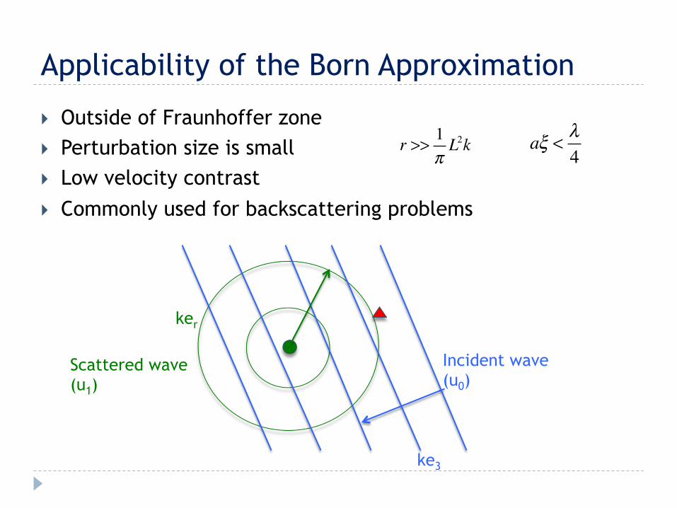
Applicability of the Born Approximation

}  Outside of Fraunhoffer zone }  Perturbation size is small }  Low velocity contrast }  Commonly used for backscattering problems

r >> 1!L2k a! < "

4

Incident wave (u0)

Scattered wave (u1)

ke3

ker

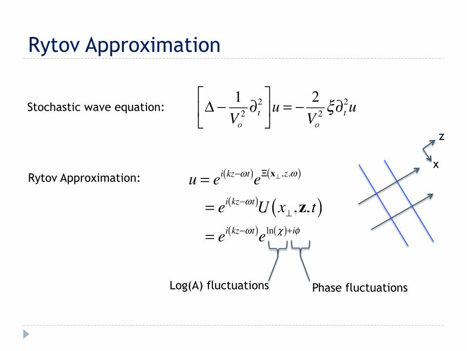
Rytov Approximation

Stochastic wave equation: ! " 1Vo2 #t

2$

%&

'

()u = " 2

Vo2 !#t

2u

Rytov Approximation: u = ei kz!!t( )e" x# ,z,!( )

= ei kz!!t( )U x#,z, t( )= ei kz!!t( )eln "( )+i#

z

x

Log(A) fluctuations Phase fluctuations

Rytov Approximation

!u = "# " Uei kz$!t( )( )( ) = %z2U + 2ik%zU $ k2U + !&U'( )*e

i kz$!t( )

%t2u = %

% t

%% t

Uei kx$!t( )( )+,-

./0 = %t

2U $ 2i!%tU $! 2U'( )*ei kz$!t( )

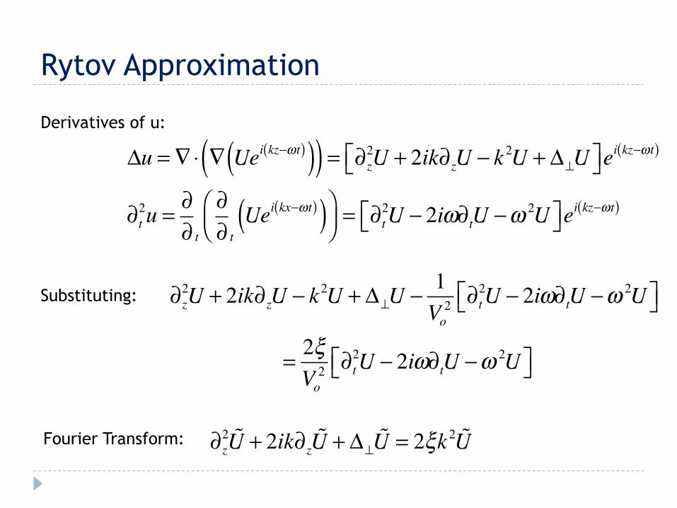
Derivatives of u:

Substituting: !z2U + 2ik!zU " k2U + #$U " 1

Vo2 !t

2U " 2i!!tU "! 2U%& '(

= 2"Vo2 !t

2U " 2i!!tU "! 2U%& '(

Fourier Transform: !z2 !U + 2ik!z !U + "#

!U = 2!k2 !U

Rytov Approximation

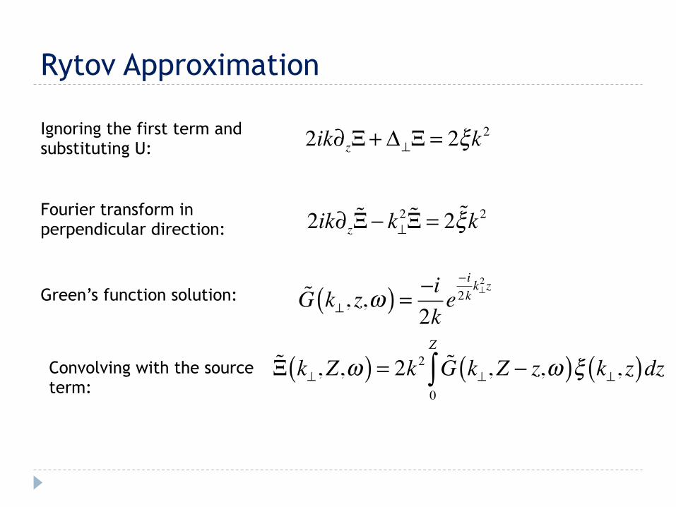
Ignoring the first term and substituting U: 2ik!z"+ #$" = 2!k2

Fourier transform in perpendicular direction: 2ik!z !"# k$

2 !" = 2 !!k2

Green’s function solution: !G k!, z,!( ) = "i2ke"i2kk!2z

Convolving with the source term:

!! k",Z,!( ) = 2k2 !G k",Z # z,!( )0

Z

$ ! k", z( )dz

Rytov Approximation:

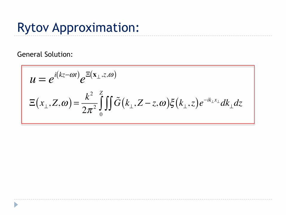
General Solution:

! x",Z,!( ) = k2

2! 2!G k",Z # z,!( )$$

0

Z

$ ! k", z( )e#ik"x"dk"dz

u = ei kz!!t( )e" x# ,z,!( )

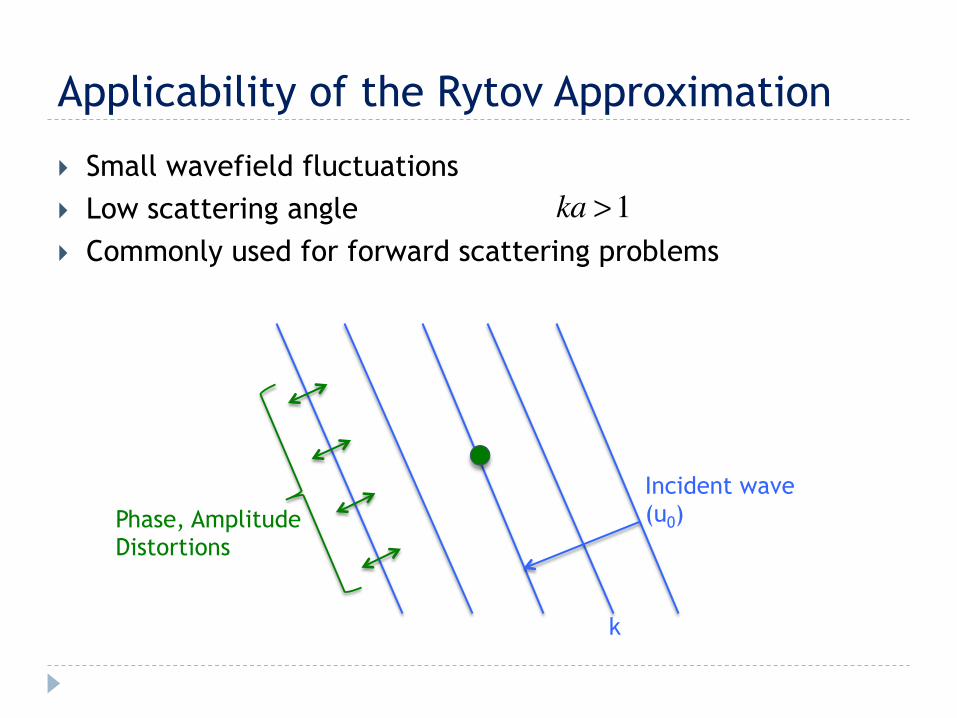
Applicability of the Rytov Approximation

}  Small wavefield fluctuations }  Low scattering angle }  Commonly used for forward scattering problems

ka >1

Incident wave (u0)

k

Phase, Amplitude Distortions

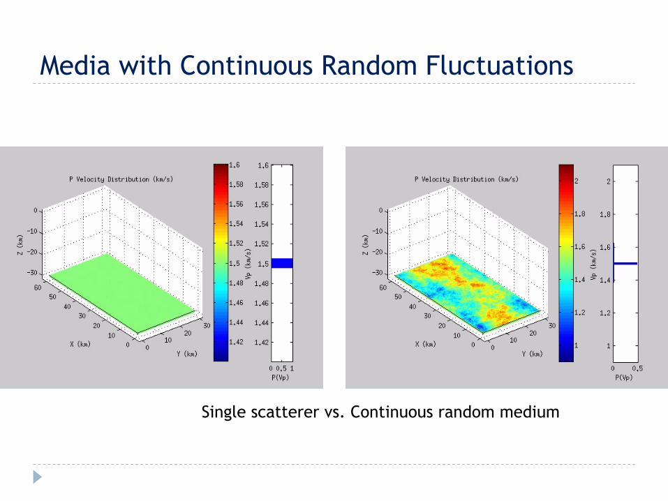
Media with Continuous Random Fluctuations

Single scatterer vs. Continuous random medium

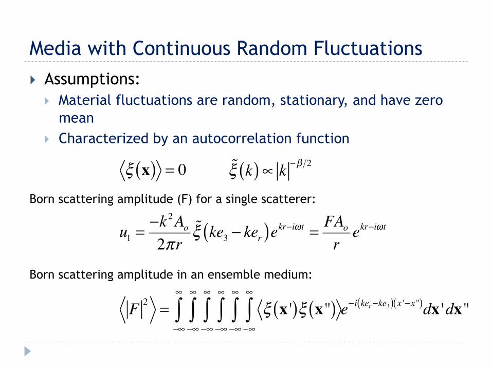
Media with Continuous Random Fluctuations }  Assumptions:

}  Material fluctuations are random, stationary, and have zero mean

}  Characterized by an autocorrelation function

u1 =!k2Ao2!r

!! ke3 ! ker( )ekr!i!t = FAorekr!i!t

Born scattering amplitude (F) for a single scatterer:

Born scattering amplitude in an ensemble medium:

F 2 = ! x '( )! x ''( )!"

"

#!"

"

#!"

"

#!"

"

#!"

"

#!"

"

# e!i ker!ke3( ) x '!x ''( )dx 'dx ''

! x( ) = 0 !! k( )! k "! 2

Most Probable Seismic Pulse

!"#$%! $& '"(")*+"# ,- +*.$(' +/" $(0")&" 12%)$") +)*(&32)!23 +/" &4"5+)%! 23 (2)!*66- #$&+)$,%+"# 7%5+%*+$2(& 89$+/ *:*%&&$*( 4)2,*,$6$+- #"(&$+- 3%(5+$2( 9$+/ ;")2 !"*( *(# %($+0*)$*(5"< !%6+$46$"# ,- +/" &=%*)" )22+ 23 +/" 7%5+%*+$2(&4"5+)%! *& #">("# $( "=& 8?@< *(# 8?A<BC( +/" 4)"&"(+ "D*!46"& 9" &$!%6*+" * 46*(" 9*0" 4)24*'*+$('

3)2! +/" +24 #29( +2 * 5")+*$( #"4+/ 8!E#$)"5+$2(< $( * &$('6")*(#2! !"#$%! )"*6$;*+$2(B F$!$6*) +)*(&!$&&$2( &$!%6*+$2(&$( *52%&+$5 )*(#2! !"#$* 9")" 4")32)!"# ,- 1*(' G H%I66")8@JJK<L F/*4$)2 "# $%& 8@JJK,< *(# F*!%"6$#"& G H%.")M$ 8@JJN<BO/" '"2!"+)- *(# +/" !"#$%! 4*)*!"+")& *)" 23 +/" 2)#") 23)"&")02$) &5*6"& *(# +/2&" 23 )"&")02$) )25.&L )"&4"5+$0"6-B O/",*5.')2%(# !"#$%! $& 5/*)*5+")$;"# ,- * 'E9*0" 0"625$+- 23PQQQ ! &!@L *( (E9*0" 0"625$+- 23 @NRQ ! &!@ *(# * #"(&$+-23 SBR ' 5!!PB C( 1$'B K 2(6- +/" /"+")2'"("2%& 4*)+ 23 +/"!2#"6 $& &/29(B C( +/" *5+%*6 1T !2#"6L 1$'B K $& "!,"##"#$( * 52(&+*(+ ,*5.')2%(# !"#$%! 9$+/ +/" 4)24")+$"& #">("#*,20"B U" 5/22&" +/" !2#"6 '"2!"+)- $( &%5/ * 9*- +/*+%(#"&$)"# )"7"5+$2(& 3)2! +/" !2#"6 ,2)#")& *)" "D56%#"#B 12)+/" !2#"66$(' 9" (""# $(&+"*# 23 0"625$+$"& +/" &+$33("&& +"(&2)52!42("(+& )@@"!#S" *(# )RR"" *(# #"(&$+- 8!L " *)" +/"V*!"W 4*)*!"+")&<B 12) &$!46$5$+-L 2(6- +/" &+$33("&& +"(&2)52!42("(+ )@@ "D/$,$+& "D42("(+$*66- 52))"6*+"# 7%5+%*+$2(&8+/" 52))"6*+$2( 6"('+/ $& AQ ! *(# +/" 52))"&42(#$(' &+*(#*)##"0$*+$2( 23 +/" 'E9*0" 0"625$+- $& @R 4") 5"(+<B U" %&" * ,2#-E32)5" 6$(" &2%)5" 9$+/ 2(6- * !E52!42("(+B X2+" +/*+ %(#")+/"&" 52(#$+$2(& (2 ( 9*0"& 9$66 ," '"(")*+"#B O/" 9*0"6"+ $&+/" &"52(# #")$0*+$0" 23 * Y$5.") 9*0"6"+ 9$+/ * #2!$(*(+3)"=%"(5- 23 *,2%+ ZR [; 8+/$& 52))"&42(#& +2 * 9*0"6"('+/ 23AQ ! 32) +/" ' 9*0"<B 1%)+/")!2)"L 9" 3%6>6 +/" &+*,$6$+- *(##$&4")&$2( 5)$+")$* )"=%$)"# 32) +/" )2+*+"# &+*''")"# ')$# *+"*5/ 42$(+ 23 +/" )*(#2! !"#$%!B O/" 9*0">"6# "(+")& +/")*(#2! !"#$%! *3+") +)*0"66$(' * 5")+*$( #$&+*(5" $( * /2!2E'"("2%& 8,*5.')2%(# "=%$0*6"(+< !"#$%!L 9/")" $+ $& *6&2)"52)#"# $( 2)#") +2 2,+*$( +/" *5+%*6 $(4%+ 9*0"6"+B

!"# $%& '()*+,-.* /0).1. .-23,0 )0+,-4+5-(2. -2 #6%*07-+

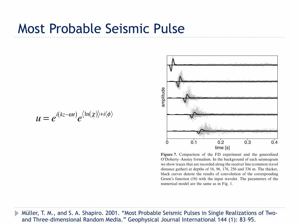
\*5/ ')"- ],*5.')2%(#^ $( 1$'B Z 52(&$&+& 23 RA +)*5"& 8+/"!E52!42("(+ 23 +/" 9*0">"6#< )"52)#"# 2( * 52!!2( +)*0"6#$&+*(5" '*+/") *+ #"4+/& 23 @KL JKL @ZKL SRK *(# PPK !B O/"#$&+*(5"& ,"+9""( '"24/2("& *62(' +/" )"5"$0") 6$(" *)" 23 +/"2)#") 23 +/" 52))"6*+$2( 6"('+/ &2 +/*+ &+*+$&+$5*66- 8&$'($>5*(+6-<#"4"(#"(+ !"*&%)"!"(+& *)" *02$#"#B 1)2! +/" %44")!2&+ +2+/" 629")!2&+ &"$&!2')*!& $( 1$'B ZL 9" 56"*)6- 2,&")0" +/*++/" *!46$+%#" *& 9"66 *& +/" +)*0"6+$!" 7%5+%*+$2(& 23 +)*5"&_)"52)#"# *+ +/" &*!" #"4+/&_$(5)"*&" 9$+/ $(5)"*&$(' +)*0"6#$&+*(5"B O/$& $& 4/-&$5*66- )"*&2(*,6" &$(5" 32) 6*)'") +)*0"6#$&+*(5"& +/")" *)" !2)" $(+")*5+$2(& 8&5*++")$(' "0"(+&< ,"+9""(+/" 9*0">"6# *(# +/" /"+")2'"("$+$"&L )"&%6+$(' $( * !2)"52!46"D 9*0">"6# *(# 52(&"=%"(+6- $( !2)" 0*)$*,6" 9*0"E32)!& *62(' +/" +)*(&0")&" #$)"5+$2( +2 +/" !*$( 4)24*'*+$2(#$)"5+$2(B X2+" +/" $(5)"*&$(' 52#*& 32) 6*)'") +)*0"6 #$&+*(5"&BO/" +/$5.") ,6*5. 5%)0" #"(2+"& +/" )"&%6+ 23 52(0260$(' +/":)""(^& 3%(5+$2( 8@N< 9$+/ +/" $(4%+ 9*0"6"+ *8#< $( +/" +$!"#2!*$(`

+!!#! !" # ,!#! !" ! *!#" " "PS#

C+ $& 2,0$2%& +/*+ +/" +/"2)"+$5*66- 4)"#$5+"# 9*0">"6# $( 1$'B Z)"4)"&"(+& +/" &$!%6*+"# 9*0">"6# $( * &2!"9/*+ &!22+/"#32)!B a%) 32)!*6$&! *6629& %& +2 !2#"6 +/" "026%+$2( 23

&"$&!$5 9*0"& $( )*(#2! !"#$* ("*) +/" >)&+ *))$0*6&B F2 3*)L9" 5*( 52(56%#" +/*+ +/" aT? 32)!*6$&! '$0"& * &!22+/"#&"$&!2')*!L *6+/2%'/ $+ $& (2+ .(29( 9/*+ .$(# 23 *0")*'$('&/2%6# ," *446$"# 8&"" *6&2 +/" ("D+ &"5+$2(L $( 9/$5/ +/")"6*+$2( +2 52!!2( *0")*'$(' 4)25"#%)"& $& #$&5%&&"#<Ba%) 9*0">"6# #"&5)$4+$2( $& ,*&"# %42( &"63E*0")*'"#

=%*(+$+$"& *(# &/2%6# ," *,6" +2 #"&5)$," +/" !2&+ 4)2,*,6"4)$!*)- *& 9"66 *& ," * '22# *44)2D$!*+$2( 32) 4)$!*)$"& $(+-4$5*6 &"$&!2')*!&B C( 2)#") +2 #"!2(&+)*+" +/$& (%!")$5*66-L9" &/2%6# 622. 32) +/" 4)2,*,$6$+- #"(&$+$"& *(# >(# +/2&"&"$&!2')*!& 9/2&" 9*0">"6# *++)$,%+"& 52$(5$#" 9$+/ +/"!*D$!* 23 +/" 4)2,*,$6$+- #"(&$+$"&B O2 #2 &2L 9" 52(&$#") +/"/$&+2')*!& 23 +/" *!46$+%#"& 32) *66 +)*5"& )"52)#"# *+ "*5/+)*0"6 #$&+*(5"B O/" /"$'/+& 23 +/" ')"- ,*)& 8255%))"(5" -< $(1$'B N #"(2+" +/" 4)2,*,$6$+- 23 2,+*$($(' &"$&!2')*!& 9$+/*!46$+%#" 0*6%"& 8*!46$+%#" 23 +/" 4)$!*)-< 9$+/$( *( $(+")0*6#"+")!$("# ,- +/" 9$#+/& 23 +/" ,*)&B O/"&" /$&+2')*!& 5*( ,">++"# 9"66 ,- * 62'E(2)!*6 4)2,*,$6$+- #"(&$+- 8,6*5. 5%)0"& $(1$'B N<B C( +/" 6$'/+ 23 +/" Y-+20 +)*(&32)!*+$2(L 62'E(2)!*6#$&+)$,%+"# *!46$+%#"& *)" +/" "D4"5+"# )"&%6+L &$(5" +/" 62'E*!46$+%#" 8*(# *6&2 4/*&"< 7%5+%*+$2(& *)" 5/*)*5+")$;"# ,- *(2)!*6 #$&+)$,%+$2( 8Y-+20 "# $%& @JNZ<B O/" +/$5. ,6*5. 0")+$5*66$("& $( 1$'B N #"(2+" +/" *!46$+%#"& 4)"#$5+"# ,- +/" :)""(^&3%(5+$2( 8@N< *(# 52$(5$#" 9$+/ +/" !*D$!* 23 +/" 4)2,*,$6$+-#"(&$+- 3%(5+$2(& 32) *66 +)*0"6 #$&+*(5"&B 1)2! +/$& 52(E&$#")*+$2( 9" 52(56%#" +/*+ +/" 4)242&"# :)""(^& 3%(5+$2( $&*,6" +2 4)"#$5+ +/" *!46$+%#"& 23 +/" 4)$!*)- *))$0*6&B[29"0")L 9" 56*$!"# +2 4)"#$5+ +/" !2&+ 4)2,*,6" 4)$!*)-

9*0">"6#B O/")"32)"L 9" &/2%6# 622. (2+ 2(6- 32) +/" !2&+4)2,*,6" *!46$+%#" ,%+ *6&2 32) +/" !2&+ 4)2,*,6" 4/*&"8+)*0"6+$!"<B b2(&+)%5+$(' +/" /$&+2')*!& 32) +/" 4/*&"&L 9"*5/$"0" * &$!$6*) )"&%6+` +/" 4/*&" 23 2%) :)""(^& 3%(5+$2(52$(5$#"& 9$+/ +/" !*D$!%! 23 +/" 4)2,*,$6$+- #"(&$+- 3%(5+$2(BO/")"32)"L 2%) :)""(^& 3%(5+$2( #"&5)$,"& * &"$&!2')*! 9/2&"*!46$+%#" *(# 4/*&" 52$(5$#" 9$+/ +/" !*D$!* 23 +/")"&4"5+$0" 4)2,*,$6$+- #"(&$+$"&B

0 0.1 0.2 0.3 0.4time [s]

ampl

itude

8-31)0 9" b2!4*)$&2( 23 +/" 1T "D4")$!"(+ *(# +/" '"(")*6$;"#a^T2/")+-c?(&+"- 32)!*6$&!B C( +/" ,*5.')2%(# 23 "*5/ &"$&!2')*!9" &/29 +)*5"& +/*+ *)" )"52)#"# *62(' +/" )"5"$0") 6$(" 852!!2( +)*0"6#$&+*(5" '*+/")< *+ #"4+/& 23 @KL JKL @ZKL SRK *(# PPK !B O/" +/$5.")L,6*5. 5%)0"& #"(2+" +/" )"&%6+& 23 52(026%+$2( 23 +/" 52))"&42(#$(':)""(^& 3%(5+$2( 8@N< 9$+/ +/" $(4%+ 9*0"6"+B O/" 4*)*!"+")& 23 +/"(%!")$5*6 !2#"6 *)" +/" &*!" *& $( 1$'B @B

JQ .& /& /+0%%"1 $23 (& 4& (5$6718

! SQQ@ Y?FL ,9: :;;< NPcJR

u = ei kz!!t( )e ln "( ) +i #

Müller, T. M., and S. A. Shapiro. 2001. “Most Probable Seismic Pulses in Single Realizations of Two- and Three-dimensional Random Media.” Geophysical Journal International 144 (1): 83–95.

Scattering Attenuation

! local =! s ! 2k2" cos # 2L / k( )"n

3D #( )0

#

$ d#

382 S. A. Shapiro and G. Kneib

18 amplitude spectra a t different distances

0 50 100 150, 200 250 300

18 amplitude spectra at different distances

P 0

W 0

N 0

c 0

0

0 50 100 150 200 250 300 frequency [Hz] frequency [Hz]

Figure 8. Meanfield amplitude spectra computed at different travel distances. The spectra have been computed from the data in Fig. 7. Spectra of the complete traces (left) are rough because the meanfield coda is not zero, i.e. spatial averaging is not perfect. Amplitude spectra of the windowed traces are smooth. The decrease and shift to lower frequencies reflects the behaviour of meanfield amplitudes. For reference the amplitude spectrum of the input wavelet is also shown.

amplitude, and resp -0.125 In 2 = -0.087 for the logarithm of the mean amplitude as expected from the theory.

In summary, we find good agreement between the theory and the numerical simulations. Small deviations from theory in Figs 7 to 14 can be explained by non-perfect averaging

and therefore can be reduced by improved spatial averaging or by ensemble averaging. Our results not only prove that our theory works but also that high-order finite difference operators can be applied to model random-media wave propagation highly accurately.

0

I 0

e

I 0 N

I 0 w

I 0

L

I 0 VI

0

I 0

0 e

I 0

0

I 0

N e

lnflA(tu>)i); f = l O O ; data=. theory=fat line

0 100 ZOO 300 400 500 800 distance [m]

ln(<lA(f)l>); f=100; data=. theory=fat line

0 100 ZOO 300 400 500 600 dlntance [m]

? co 0

I ; I 0

0

I 0

N e

<ln(lA(f)l)>; f=100; date=. theory=fat line

0 100 200 300 400 600 600 dintance [m]

i ( < l A ( f ) [ * * Z > ) ; f = 100; data=.

. .

I 100 200 300 400 500 600

distance [m]

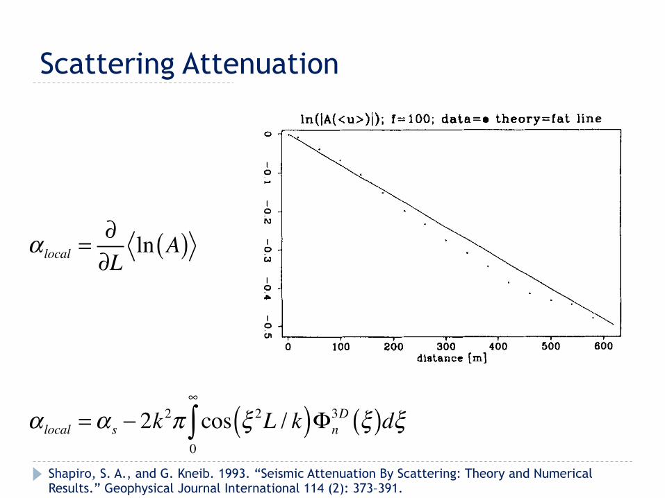
Figure 9. In /(u)l (top, left), (In A ) (top, right), In (A ) (bottom, left), and In (A2) (bottom, right) for the dominant frequency of 100 Hz. Points denote the numerical experiment, solid lines denote theory. The bent curve in the Figures of (In A) and In (A) refers to the weak fluctuation region and the horizontal line to the strong fluctuation region.

! local =!!L

ln A( )

Shapiro, S. A., and G. Kneib. 1993. “Seismic Attenuation By Scattering: Theory and Numerical Results.” Geophysical Journal International 114 (2): 373–391.

Phase velocity in random media 791

1.4

0.8

0.6

0.4

theory (10%) - expenment (10%) 0

theory (5%) experiment (5%) +

theory (3%) - expenment (3%) 0

1 1.5 2 2.5 3 3.5 4 4.5 5 5.5 Wa

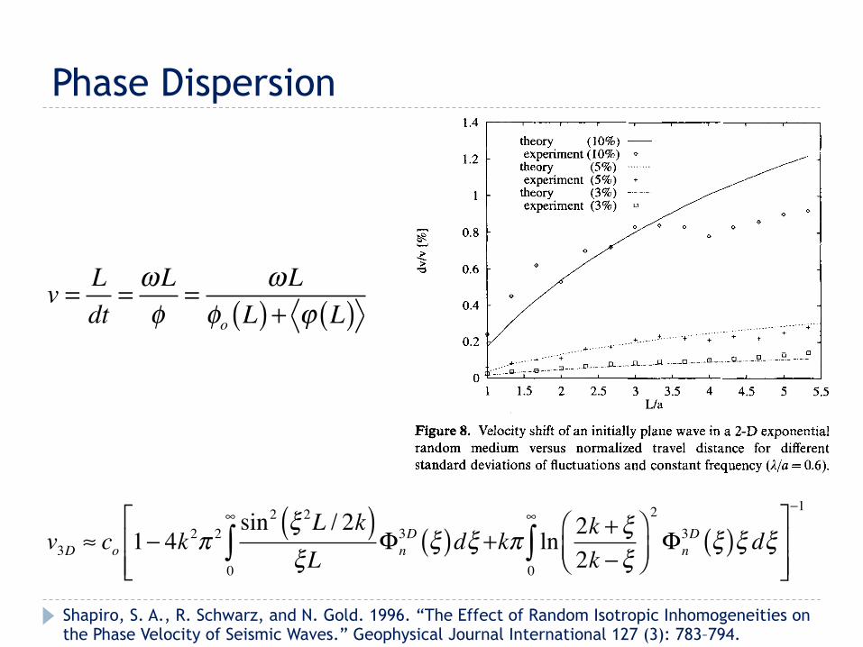
Figure 8. Velocity shift of an initially plane wave in a 2-D exponential random medium versus normalized travel distance for different standard deviations of fluctuations and constant frequency (A/a = 0.6).

1.6

1.4

1.2

1

> 0.8

- E . a

0.6

0.4

0.2

0

Huygens method ~

theory @ l a = 0.1) expenment (h /a = 0.625) o

theory (hla = 0.625) experiment (hla = 1) +

theory (h /a=1) - - -

1 1.5 2 2.5 3 3.5 4 4.5 5 5.5 6 L/a

Figure 9. Velocity shift of an initially plane wave in a 2-D exponential random medium versus normalized travel distance for different fre- quencies and a constant standard deviation of fluctuations (5 per cent). The curve computed by the Huygens method has been taken from Fig. 8 of Roth et al. (1993).

fluctuations is 5 per cent. Good agreement between theoretical and numerical results is observed. For comparison, the results of the high-frequency asymptotic calculations of Roth et al. (1993) are also shown in Fig. 9. The major importance of the frequency dependence of the effect is evident.

Finally, Fig. 10 provides the theoretical results in the case of 3-D inhomogeneous exponential media that have the same statistical parameters as the 2-D models described above. This figure should be compared with Fig. 8. One can see a consider- able increase of the velocity shift in 3-D media in comparison with 2-D media.

CONCLUSIONS

In 2-D and 3-D random media the phase velocity is not only frequency-dependent, but travel-distance-dependent as well. This dependence becomes unimportant in the frequency range which can be approximately given by the inequality ka 5 5. Moreover, in the low-frequency range the velocity shift

1.8

c

E > a .

1 1.5 2 2.5 3 3.5 4 4.5 5 5.5 L / a

Figure 10. Velocity shift of initially plane waves in 3-D exponential media for different variances of velocity fluctuations of l / a = 0.6.

becomes negative. With increasing L/a the dispersion becomes larger. It is important for the intermediate-frequency range, which can be approximately expressed as 1 < ka 5 10 L/a. In realistic cases the shift of the observed phase velocity relative to the reciprocal averaged slowness is smaller than 2 per cent. The frequency dependence of the velocity shift can be very strong. Therefore, the results of ray-perturbation theory and other high-frequency approximations may be non-applicable in relevant frequency- and travel-distance domains. Moreover, ray-perturbation theory is not able to describe the effect of fractal-like inhomogeneities. Here we have presented a theory that describes the frequency- and travel-distance dependences of the phase velocity of the transmitted wavefield. The low- frequency limit of our analytical results coincides with the known effective-medium limit of the phase velocity in statistically isotropic inhomogeneous fluids with constant densities. In the high-frequency limit our results coincide with the result pre- viously obtained by ray-perturbation theory. Our theory is, however, also valid in the case of media with non-differentiable autocorrelation functions (e.g. media with exponential auto- correlation functions or fractal media). Its results agree well with numerical simulations.

ACKNOWLEDGMENTS

We thank Michael Roth, Michael Korn and Gerhard Muller for their discussions and comments, which greatly improved the manuscript. This research was partly supported by the Deutsche Forchungsgemeinschaft in the framework of the research program SFB 381. This is Karlsruhe University Geophysical Institute publication N 675.

REFERENCES

Gradshteyn, IS. & Ryzhik, I.M., 1983. Table of Integrals, Series and Products, Academic Press, London.

Ikelle, L.T. & Yung, S.K., 1994. An example of lateral-inhomogeneity effects on seismic traveltimes in a zero-offset VSP experiment, Geophys. 3. Int., 118, 802-807.

Ishimaru, A., 1978. Wave Propagation and Scattering in Random Media, Academic Press, New York, NY.

Kneib, G. & Kerner, C., 1993. Accurate and efficient seismic modeling in random media, Geophysics, 58, 576-588.

0 1996 RAS, GJI 127, 783-794

Phase Dispersion

v = Ldt

= !L!

= "L!o L( )+ ! L( )

v3D ! co 1" 4k2! 2 sin2 " 2L / 2k( )

!L#n3D !( )d!

0

$

%&

'((

+k" ln 2k +!2k "!

)*+

,-.

2

#n3D !( )! d!

0

$

%/

011

"1

Shapiro, S. A., R. Schwarz, and N. Gold. 1996. “The Effect of Random Isotropic Inhomogeneities on the Phase Velocity of Seismic Waves.” Geophysical Journal International 127 (3): 783–794.

Inverting for Distribution Parameters

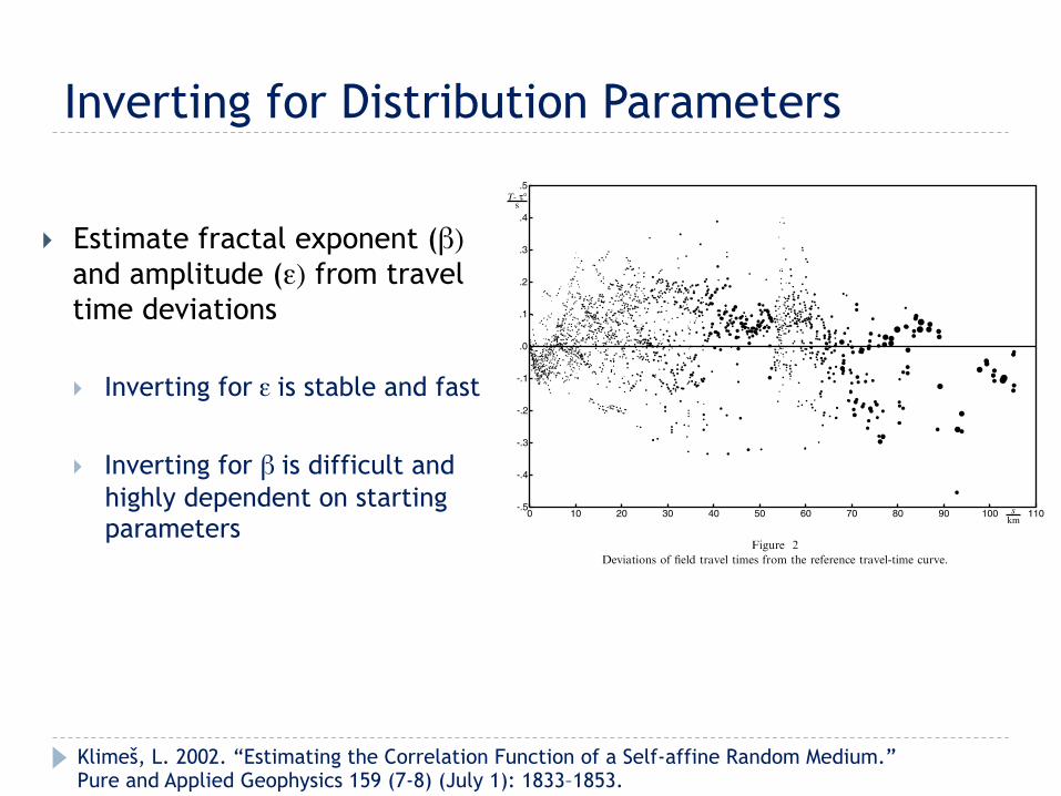
}  Estimate fractal exponent (β) and amplitude (ε) from travel time deviations

}  Inverting for ε is stable and fast

}  Inverting for β is difficult and highly dependent on starting parameters

to achieve a relatively even coverage of all hypocentral distances s. The squared

travel-time deviations have then been weighted with the least-squares weights

w00K ! w0

Ks"p where p ! 0:5 : #65$

5.2. Calculation of Covariances between Travel Times

For the estimation of the parameters of the medium correlation function, we

consider straight rays, as in a homogeneous medium. For the used refraction traveltimes whose rays do not penetrate the earth very deeply compared with the

epicentral distance, it should be a reasonable approximation. Especially if the rays ofconsiderably di!erent lengths are not compared, see condition (34).

Geometrical covariance matrix (25) of travel times has been calculated numer-

ically, dividing the rectangular integration area of dimensions sK % sL into smallrectangular cells and replacing the integrand by a bilinear function in each cell. Since

the integrand may reach infinity at some points, the integrand has been limited fromabove at each grid point in such a way as to secure exact values of the integral in all

square cells touched by the diagonal for the special case of variances HKK .Unfortunately, the first version of the code used for these tests is not su"ciently

debugged, is slow and not su"ciently accurate. This may influence the reliability of

Figure 2Deviations of field travel times from the reference travel-time curve.

1846 Ludek Klimes Pure appl. geophys.,

Klimeš, L. 2002. “Estimating the Correlation Function of a Self-affine Random Medium.” Pure and Applied Geophysics 159 (7-8) (July 1): 1833–1853.

Issues with Born and Rytov Approximation }  Single scattering }  Does not conserve energy }  Does not take into account near-field effects

}  Effective shear energy ~10% of compressional wave energy is not accounted for… (My research is looking into this)

}  Other methods: }  Radiative Transfer Theory }  Finite Difference / Finite Element

Sato, Haruo, Michael C. Fehler, and Takuto Maeda. 2012. Seismic Wave Propagation and Scattering in the Heterogeneous Earth : Second Edition. Springer.

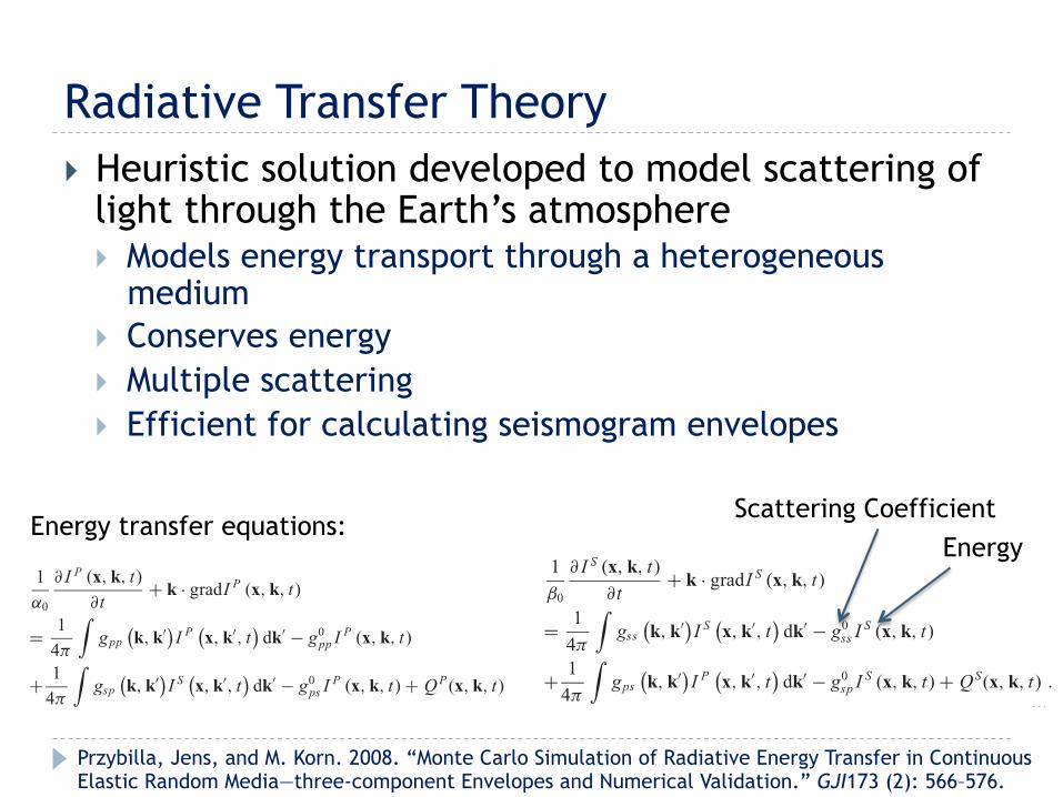
Radiative Transfer Theory }  Heuristic solution developed to model scattering of

light through the Earth’s atmosphere }  Models energy transport through a heterogeneous

medium }  Conserves energy }  Multiple scattering }  Efficient for calculating seismogram envelopes

Energy transfer equations:

Monte Carlo solutions of the 3-D RT equations 567

isotropic scattering and scalar waves in a background medium witha velocity gradient with depth, which can be implemented by mov-ing the particles along curved ray trajectories between scatteringevents. Wegler et al. (2006) compared the performance of isotropicand non-isotropic scattering approximations for scalar waves andfound that isotropic scattering yields considerable deviations in theearly parts of the coda. Margerin et al. (2000), for the first time, de-veloped a Monte Carlo scheme for the full elastic vector wave casein a medium with discrete scatterers, where conversions between P-and S-wave modes are taken into account, and the S-wave polariza-tion is taken care of with the help of the Stokes vector. Elastic RThas been applied to deep mantle scattering (Margerin & Nolet 2003;Shearer & Earle 2004).

Przybilla et al. (2006) proposed a RT scheme for elastic vec-tor waves in 2-D continuous random media employing angular-dependent scattering patterns described by Born scattering coef-ficients (Sato & Fehler 1998). They tested the accuracy of envelopeshapes against averaged envelopes from full waveform modellingwith a finite-difference (FD) method and found that RT yields ac-curate envelope shapes for a wide range of medium parameters,including strong forward scattering cases.

In this paper we extend the 2-D method of Przybilla et al. (2006)to three dimensions. We avoid introducing the Stokes vector andinstead use the polarization decomposed Born scattering coeffi-cients to carry the polarization information of S-wave particlesacross scattering events. The method enables us to model com-plete three-component mean square envelopes in random mediawith prescribed autocorrelation functions from the first P onset untilthe late S coda. Thus, this method is more powerful than diffusionapproaches, which only model late S coda, and the Markov ap-proximation, which is only valid around the ballistic direct wavearrivals, and more accurate than multiple scattering methods withisotropic scattering assumptions. We expect that by inverting com-plete seismogram envelopes, we will get more reliable informationon the statistics of the propagation media than by using only scalarapproximation to model the S-wave envelopes.

Similarly to Przybilla et al. (2006), we demonstrate the accu-racy of our approach by comparing it to average envelope shapesfrom full 3-D elastic waveform modelling. We further compare thepulse broadening effect for strong forward scattering with the newlydeveloped Markov approximation for vector waves (Sato 2007).

2 E L A S T I C R A D I AT I V E T R A N S F E RT H E O RY

2.1 Basic equations

For a detailed derivation of RT equations from wave theory in ran-dom media, we refer to Ryzhik et al. (1996). The key quantity inthis theory is the specific intensity I(x, k, t) of a wave at point x,time t, moving in direction k. Here we introduce specific intensitiesIp and Is for P and S waves, respectively. Following Ryzhik et al.(1996) the coupled elastic energy transfer equations for Ip and Is

can be written as

1!0

" I P (x, k, t)"t

+ k · gradI P (x, k, t)

= 14#

!gpp

"k, k!#I P

"x, k!, t

#dk! " g0

pp I P (x, k, t)

+ 14#

!gsp

"k, k!#I S

"x, k!, t

#dk! " g0

ps I P (x, k, t) + Q P (x, k, t)

1$0

" I S (x, k, t)"t

+ k · gradI S (x, k, t)

= 14#

!gss

"k, k!#I S

"x, k!, t

#dk! " g0

ss I S (x, k, t)

+ 14#

!gps

"k, k!#I P

"x, k!, t

#dk! " g0

sp I S (x, k, t) + QS(x, k, t) .

(1)

In eq. (1) unit wavenumber k denotes incident wave direction andk!, any other direction. !0 and $ 0 are the mean P and S velocities.gij and gij

0 (i, j = P or S) are angular-dependent and total scatteringcoefficients (see below), respectively. The left-hand side of eq. (1)represents the total time derivative of intensities and describes theintensity transport of P and S waves. The right-hand side containsthe intensity loss from the direction of propagation into all otherdirections k! through the total scattering coefficients gij

0, and theintensity gain from all directions into the propagation direction kthrough the integral over gij. Conversion scattering between P and Senergy is contained in gps and gsp and couples both equations. Q P,S

(x, k, t) represent sources of P and S waves.The basic assumptions of RTT are: (1) fluctuations of the inho-

mogeneities are weak; (2) wavelength and correlation length of theheterogeneities are of comparable size and (3) phases of waves fromdifferent scattereres are independent of each other, that is, the energyof scattered wave packets can be stacked (Rhyzhik et al. 1996). Thisis often casted into the condition (ka%)2 # 1 (Apresyan & Kravtsov1996, p. 184; Gusev & Abubakirov 1996). Energy dissipation andvelocity dispersion are neglected in eq. (1).

2.2 Scattering coefficients

For determination of the scattering coefficients gij in eq. (1), we usethe random medium model with continuous velocity and densityfluctuations with respect to a constant background model !0, $ 0

and density & 0. Here we use the assumption (e.g. Sato & Fehler1998, p. 101) that P- and S-wave velocity fluctuations are propor-tional to each other and that wave velocity and density follow alinear relationship (Birch 1961). Then the number of independentfractional fluctuations is reduced to one spatially stationary randomvariable ' (x):

(!

!0= ($

$0= 1

)

(&

&0= ' (x) . (2)

Useful values for ) are in the range 0.3–0.8. The statistics of themedium is given by the autocorrelation function

R(x) = $' (x + x!)' (x!)%, (3)

and variance

%2 = R(0) = $' (x)2%. (4)

The power spectrum of the medium at wavenumber m is obtainedby a Fourier transform of R as

P (m) =! ! !

R (x)e"im·xdx. (5)

Coefficients gij describe single scattering interactions of wavepackets with the random heterogeneities and can be obtained withinthe framework of Born approximation (e.g. Sato & Fehler 1998,p. 95ff). Many previous RT solutions have assumed average,direction-independent values for these coefficients. Although thisis a reasonable assumption in the Rayleigh scattering domain whenthe correlation distance of heterogeneities is much smaller than the

C& 2008 The Authors, GJI, 173, 566–576Journal compilation C& 2008 RAS

Monte Carlo solutions of the 3-D RT equations 567

isotropic scattering and scalar waves in a background medium witha velocity gradient with depth, which can be implemented by mov-ing the particles along curved ray trajectories between scatteringevents. Wegler et al. (2006) compared the performance of isotropicand non-isotropic scattering approximations for scalar waves andfound that isotropic scattering yields considerable deviations in theearly parts of the coda. Margerin et al. (2000), for the first time, de-veloped a Monte Carlo scheme for the full elastic vector wave casein a medium with discrete scatterers, where conversions between P-and S-wave modes are taken into account, and the S-wave polariza-tion is taken care of with the help of the Stokes vector. Elastic RThas been applied to deep mantle scattering (Margerin & Nolet 2003;Shearer & Earle 2004).

Przybilla et al. (2006) proposed a RT scheme for elastic vec-tor waves in 2-D continuous random media employing angular-dependent scattering patterns described by Born scattering coef-ficients (Sato & Fehler 1998). They tested the accuracy of envelopeshapes against averaged envelopes from full waveform modellingwith a finite-difference (FD) method and found that RT yields ac-curate envelope shapes for a wide range of medium parameters,including strong forward scattering cases.

In this paper we extend the 2-D method of Przybilla et al. (2006)to three dimensions. We avoid introducing the Stokes vector andinstead use the polarization decomposed Born scattering coeffi-cients to carry the polarization information of S-wave particlesacross scattering events. The method enables us to model com-plete three-component mean square envelopes in random mediawith prescribed autocorrelation functions from the first P onset untilthe late S coda. Thus, this method is more powerful than diffusionapproaches, which only model late S coda, and the Markov ap-proximation, which is only valid around the ballistic direct wavearrivals, and more accurate than multiple scattering methods withisotropic scattering assumptions. We expect that by inverting com-plete seismogram envelopes, we will get more reliable informationon the statistics of the propagation media than by using only scalarapproximation to model the S-wave envelopes.

Similarly to Przybilla et al. (2006), we demonstrate the accu-racy of our approach by comparing it to average envelope shapesfrom full 3-D elastic waveform modelling. We further compare thepulse broadening effect for strong forward scattering with the newlydeveloped Markov approximation for vector waves (Sato 2007).

2 E L A S T I C R A D I AT I V E T R A N S F E RT H E O RY

2.1 Basic equations

For a detailed derivation of RT equations from wave theory in ran-dom media, we refer to Ryzhik et al. (1996). The key quantity inthis theory is the specific intensity I(x, k, t) of a wave at point x,time t, moving in direction k. Here we introduce specific intensitiesIp and Is for P and S waves, respectively. Following Ryzhik et al.(1996) the coupled elastic energy transfer equations for Ip and Is

can be written as

1!0

" I P (x, k, t)"t

+ k · gradI P (x, k, t)

= 14#

!gpp

"k, k!#I P

"x, k!, t

#dk! " g0

pp I P (x, k, t)

+ 14#

!gsp

"k, k!#I S

"x, k!, t

#dk! " g0

ps I P (x, k, t) + Q P (x, k, t)

1$0

" I S (x, k, t)"t

+ k · gradI S (x, k, t)

= 14#

!gss

"k, k!#I S

"x, k!, t

#dk! " g0

ss I S (x, k, t)

+ 14#

!gps

"k, k!#I P

"x, k!, t

#dk! " g0

sp I S (x, k, t) + QS(x, k, t) .

(1)

In eq. (1) unit wavenumber k denotes incident wave direction andk!, any other direction. !0 and $ 0 are the mean P and S velocities.gij and gij

0 (i, j = P or S) are angular-dependent and total scatteringcoefficients (see below), respectively. The left-hand side of eq. (1)represents the total time derivative of intensities and describes theintensity transport of P and S waves. The right-hand side containsthe intensity loss from the direction of propagation into all otherdirections k! through the total scattering coefficients gij

0, and theintensity gain from all directions into the propagation direction kthrough the integral over gij. Conversion scattering between P and Senergy is contained in gps and gsp and couples both equations. Q P,S

(x, k, t) represent sources of P and S waves.The basic assumptions of RTT are: (1) fluctuations of the inho-

mogeneities are weak; (2) wavelength and correlation length of theheterogeneities are of comparable size and (3) phases of waves fromdifferent scattereres are independent of each other, that is, the energyof scattered wave packets can be stacked (Rhyzhik et al. 1996). Thisis often casted into the condition (ka%)2 # 1 (Apresyan & Kravtsov1996, p. 184; Gusev & Abubakirov 1996). Energy dissipation andvelocity dispersion are neglected in eq. (1).

2.2 Scattering coefficients

For determination of the scattering coefficients gij in eq. (1), we usethe random medium model with continuous velocity and densityfluctuations with respect to a constant background model !0, $ 0

and density & 0. Here we use the assumption (e.g. Sato & Fehler1998, p. 101) that P- and S-wave velocity fluctuations are propor-tional to each other and that wave velocity and density follow alinear relationship (Birch 1961). Then the number of independentfractional fluctuations is reduced to one spatially stationary randomvariable ' (x):

(!

!0= ($

$0= 1

)

(&

&0= ' (x) . (2)

Useful values for ) are in the range 0.3–0.8. The statistics of themedium is given by the autocorrelation function

R(x) = $' (x + x!)' (x!)%, (3)

and variance

%2 = R(0) = $' (x)2%. (4)

The power spectrum of the medium at wavenumber m is obtainedby a Fourier transform of R as

P (m) =! ! !

R (x)e"im·xdx. (5)

Coefficients gij describe single scattering interactions of wavepackets with the random heterogeneities and can be obtained withinthe framework of Born approximation (e.g. Sato & Fehler 1998,p. 95ff). Many previous RT solutions have assumed average,direction-independent values for these coefficients. Although thisis a reasonable assumption in the Rayleigh scattering domain whenthe correlation distance of heterogeneities is much smaller than the

C& 2008 The Authors, GJI, 173, 566–576Journal compilation C& 2008 RAS

Przybilla, Jens, and M. Korn. 2008. “Monte Carlo Simulation of Radiative Energy Transfer in Continuous Elastic Random Media—three-component Envelopes and Numerical Validation.” GJI173 (2): 566–576.

Scattering Coefficient Energy

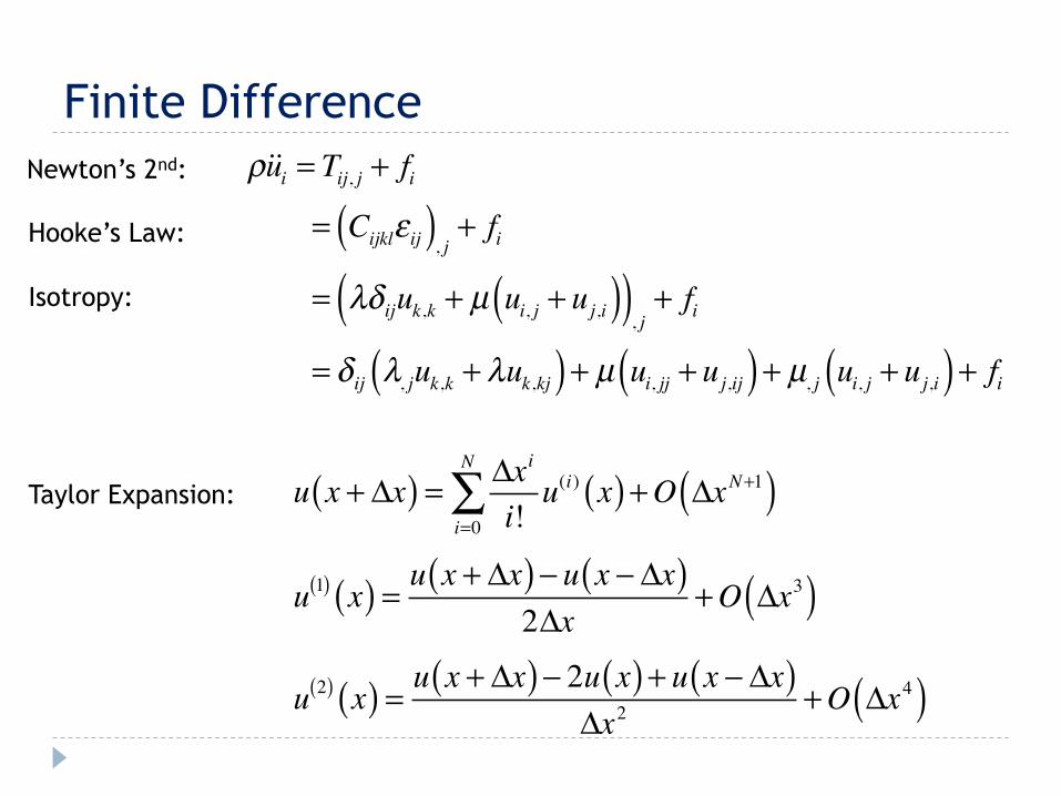
Finite Difference !!!ui = Tij, j + fi

= Cijkl! ij( ), j + fi

= !" ijuk,k + µ ui, j + uj,i( )( ), j+ fi

= ! ij !, juk,k + !uk,kj( )+ µ ui, jj + uj,ij( )+ µ, j ui, j + uj,i( )+ fi

Newton’s 2nd:

Hooke’s Law:

Isotropy:

Taylor Expansion: u x + !x( ) = !xi

i!u(i) x( )

i=0

N

" +O !xN+1( )

u 1( ) x( ) = u x + !x( )" u x " !x( )2!x

+O !x3( )

u 2( ) x( ) = u x + !x( )" 2u x( )+ u x " !x( )!x2

+O !x4( )

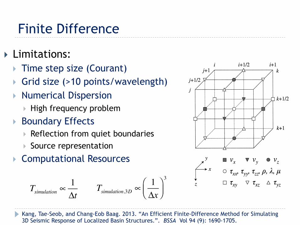
Finite Difference

}  Limitations: }  Time step size (Courant) }  Grid size (>10 points/wavelength) }  Numerical Dispersion

}  High frequency problem

}  Boundary Effects }  Reflection from quiet boundaries }  Source representation

}  Computational Resources

Tsimulation,3D ! 1"x

#$%

&'(3

Tsimulation !1"t

Kang, Tae-Seob, and Chang-Eob Baag. 2013. “An Efficient Finite-Difference Method for Simulating 3D Seismic Response of Localized Basin Structures.”. BSSA Vol 94 (9): 1690-1705.