Electroweak Symmetry Breaking (EWSB): The Basics

Howard E. Haber 23—24 July 2012

Lecture 2

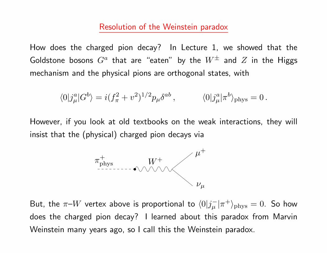
Resolution of the Weinstein paradox

How does the charged pion decay? In Lecture 1, we showed that the

Goldstone bosons Ga that are “eaten” by the W± and Z in the Higgs

mechanism and the physical pions are orthogonal states, with

〈0|jaµ|Gb〉 = i(f2

π + v2)1/2pµδab , 〈0|jaµ|πb〉phys = 0 .

However, if you look at old textbooks on the weak interactions, they will

insist that the (physical) charged pion decays via

π+phys W+

µ+

νµ

But, the π–W vertex above is proportional to 〈0|j−µ |π+〉phys = 0. So how

does the charged pion decay? I learned about this paradox from Marvin

Weinstein many years ago, so I call this the Weinstein paradox.

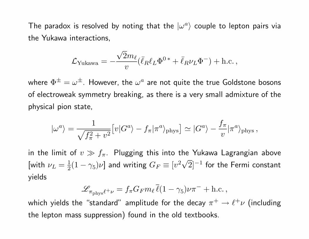
The paradox is resolved by noting that the |ωa〉 couple to lepton pairs via

the Yukawa interactions,

LYukawa = −√

2m`

v(¯R`LΦ0 ∗ + ¯

RνLΦ−) + h.c. ,

where Φ± = ω±. However, the ωa are not quite the true Goldstone bosons

of electroweak symmetry breaking, as there is a very small admixture of the

physical pion state,

|ωa〉 =1

√

f2π + v2

[

v|Ga〉 − fπ|πa〉phys

]

' |Ga〉 − fπ

v|πa〉phys ,

in the limit of v � fπ. Plugging this into the Yukawa Lagrangian above

[with νL = 12(1 − γ5)ν] and writing GF ≡ [v2

√2]−1 for the Fermi constant

yields

Lπphys`+ν = fπGFm` `(1 − γ5)νπ− + h.c. ,

which yields the “standard” amplitude for the decay π+ → `+ν (including

the lepton mass suppression) found in the old textbooks.

Lecture II

Electroweak symmetry breaking after 4 July 2012

Outline

• Phenomenology of the Standard Model (SM) Higgs boson

• The LHC discovery of 4 July 2012

• Hints of the Standard Model demise?

• Non-minimal Higgs sectors

• How unlikely is the Higgs boson?

• The significance of the TeV-scale–Part II

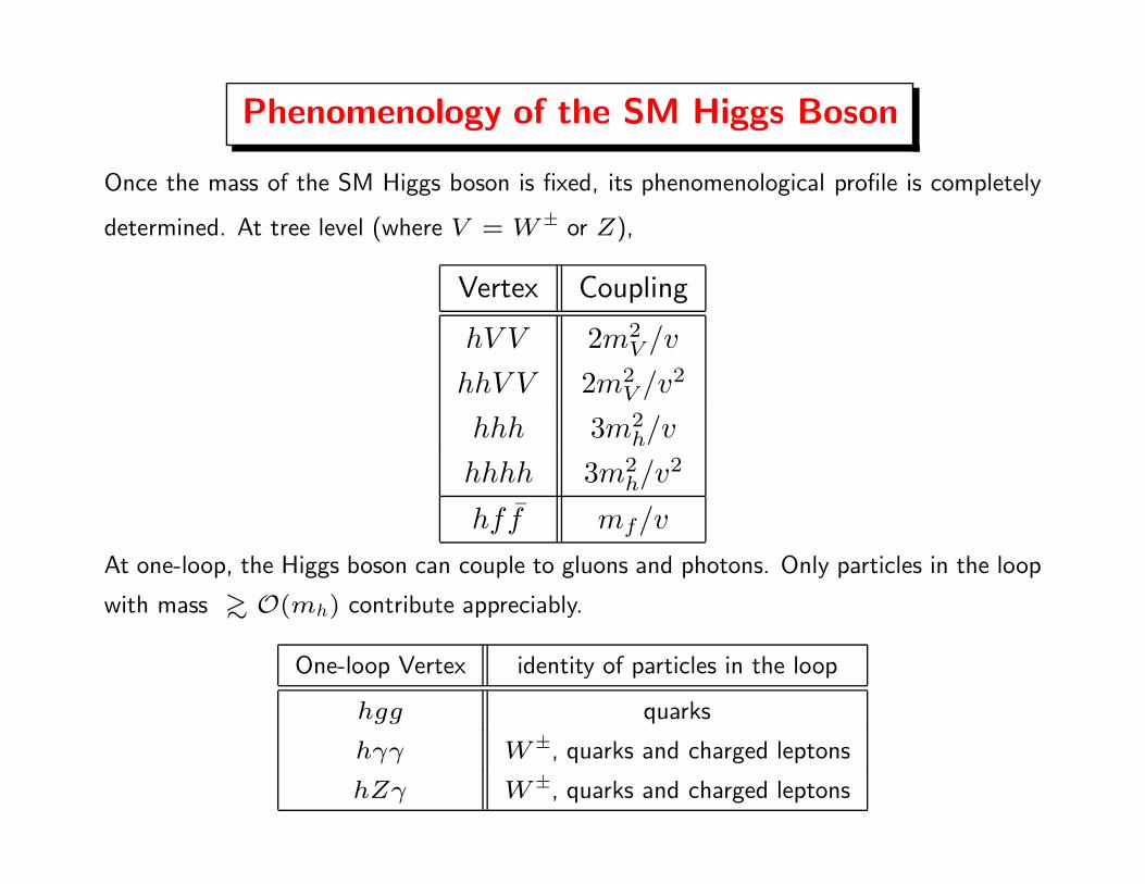
Phenomenology of the SM Higgs Boson

Once the mass of the SM Higgs boson is fixed, its phenomenological profile is completely

determined. At tree level (where V = W± or Z),

Vertex Coupling

hV V 2m2V /v

hhV V 2m2V /v2

hhh 3m2h/v

hhhh 3m2h/v2

hff mf/v

At one-loop, the Higgs boson can couple to gluons and photons. Only particles in the loop

with mass >∼ O(mh) contribute appreciably.

One-loop Vertex identity of particles in the loop

hgg quarks

hγγ W±, quarks and charged leptons

hZγ W±, quarks and charged leptons

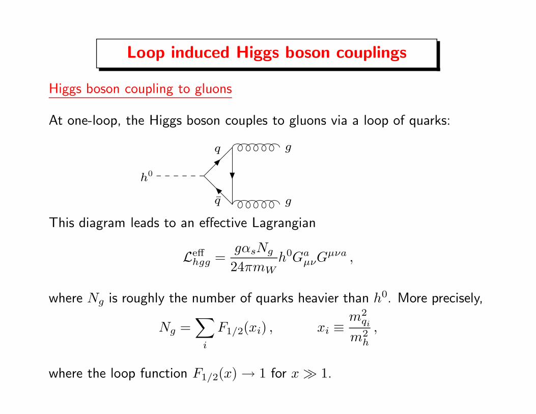
Loop induced Higgs boson couplings

Higgs boson coupling to gluons

At one-loop, the Higgs boson couples to gluons via a loop of quarks:

h0

g

g

q

q

This diagram leads to an effective Lagrangian

Leffhgg =

gαsNg

24πmWh0Ga

µνGµνa ,

where Ng is roughly the number of quarks heavier than h0. More precisely,

Ng =∑

i

F1/2(xi) , xi ≡m2

qi

m2h

,

where the loop function F1/2(x) → 1 for x � 1.

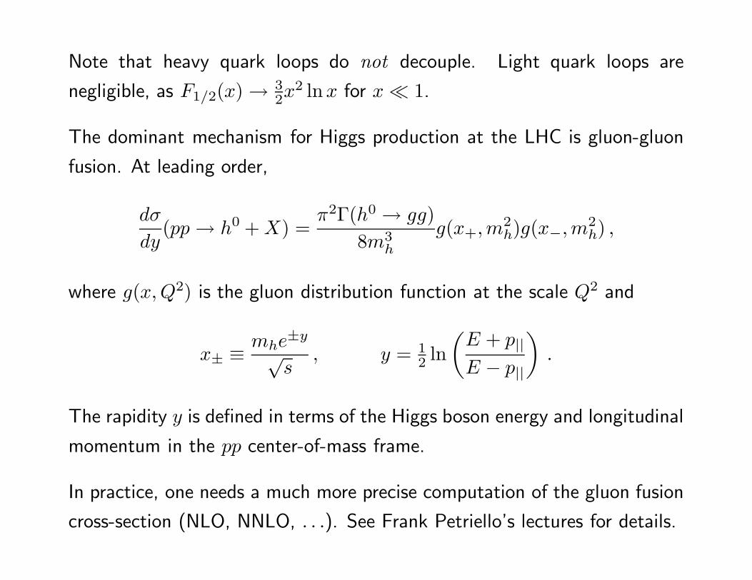
Note that heavy quark loops do not decouple. Light quark loops are

negligible, as F1/2(x) → 32x

2 lnx for x � 1.

The dominant mechanism for Higgs production at the LHC is gluon-gluon

fusion. At leading order,

dσ

dy(pp → h0 + X) =

π2Γ(h0 → gg)

8m3h

g(x+,m2h)g(x−,m2

h) ,

where g(x, Q2) is the gluon distribution function at the scale Q2 and

x± ≡ mhe±y

√s

, y = 12 ln

(

E + p||E − p||

)

.

The rapidity y is defined in terms of the Higgs boson energy and longitudinal

momentum in the pp center-of-mass frame.

In practice, one needs a much more precise computation of the gluon fusion

cross-section (NLO, NNLO, . . .). See Frank Petriello’s lectures for details.

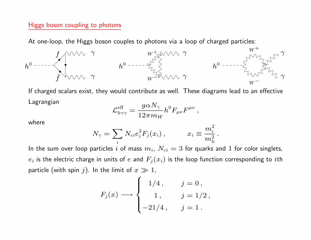
Higgs boson coupling to photons

At one-loop, the Higgs boson couples to photons via a loop of charged particles:

h0

γ

γ

f

f

h0

γ

γ

W+

W−

h0

γ

γ

W+

W−

If charged scalars exist, they would contribute as well. These diagrams lead to an effective

Lagrangian

Leffhγγ =

gαNγ

12πmW

h0FµνFµν ,

where

Nγ =X

i

Ncie2i Fj(xi) , xi ≡

m2i

m2h

.

In the sum over loop particles i of mass mi, Nci = 3 for quarks and 1 for color singlets,

ei is the electric charge in units of e and Fj(xi) is the loop function corresponding to ith

particle (with spin j). In the limit of x � 1,

Fj(x) −→

8>>><>>>:

1/4 , j = 0 ,

1 , j = 1/2 ,

−21/4 , j = 1 .

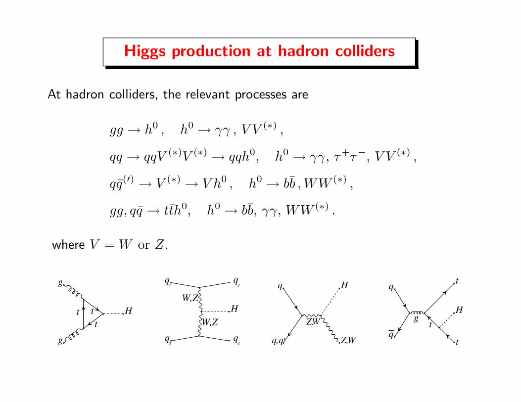
Higgs production at hadron colliders

At hadron colliders, the relevant processes are

gg → h0 , h0 → γγ , V V (∗) ,

qq → qqV (∗)V (∗) → qqh0, h0 → γγ, τ+τ−, V V (∗) ,

qq(′) → V (∗) → V h0 , h0 → bb , WW (∗) ,

gg, qq → tth0, h0 → bb, γγ, WW (∗) .

where V = W or Z.

g

g

Ht t

t

q1

q2

H

q3

q4

W,Z

W,Z

q

q, ,q

H

Z,W

Z,W

q

q

t

H

t

gt

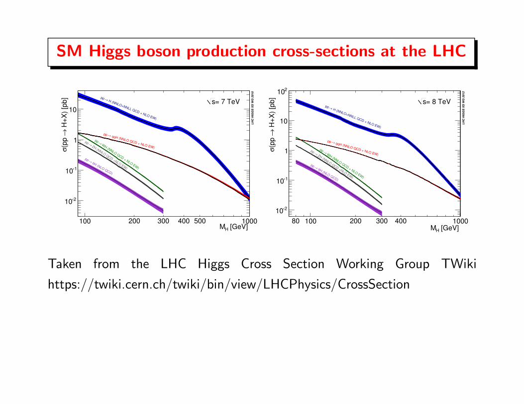
SM Higgs boson production cross-sections at the LHC

[GeV] HM100 200 300 400 500 1000

H+

X)

[pb]

→(p

p

σ

›210

›110

1

10= 7 TeVs

LH

C H

IGG

S X

S W

G 2

01

0

H (NNLO+NNLL QCD + NLO EW)

→pp

qqH (NNLO QCD + NLO EW)

→pp

WH (NNLO QCD + NLO EW

)

→pp

ZH (NNLO QCD +NLO EW)

→pp

ttH (NLO QCD)

→pp

[GeV] HM80 100 200 300 400 1000

H+

X)

[pb]

→(p

p

σ

›210

›110

1

10

210

= 8 TeVs

LH

C H

IGG

S X

S W

G 2

01

2

H (NNLO+NNLL QCD + NLO EW)

→pp

qqH (NNLO QCD + NLO EW)

→pp

WH (NNLO QCD + NLO EW

)

→pp

ZH (NNLO QCD +NLO EW)

→pp

ttH (NLO QCD)

→pp

Taken from the LHC Higgs Cross Section Working Group TWiki

https://twiki.cern.ch/twiki/bin/view/LHCPhysics/CrossSection

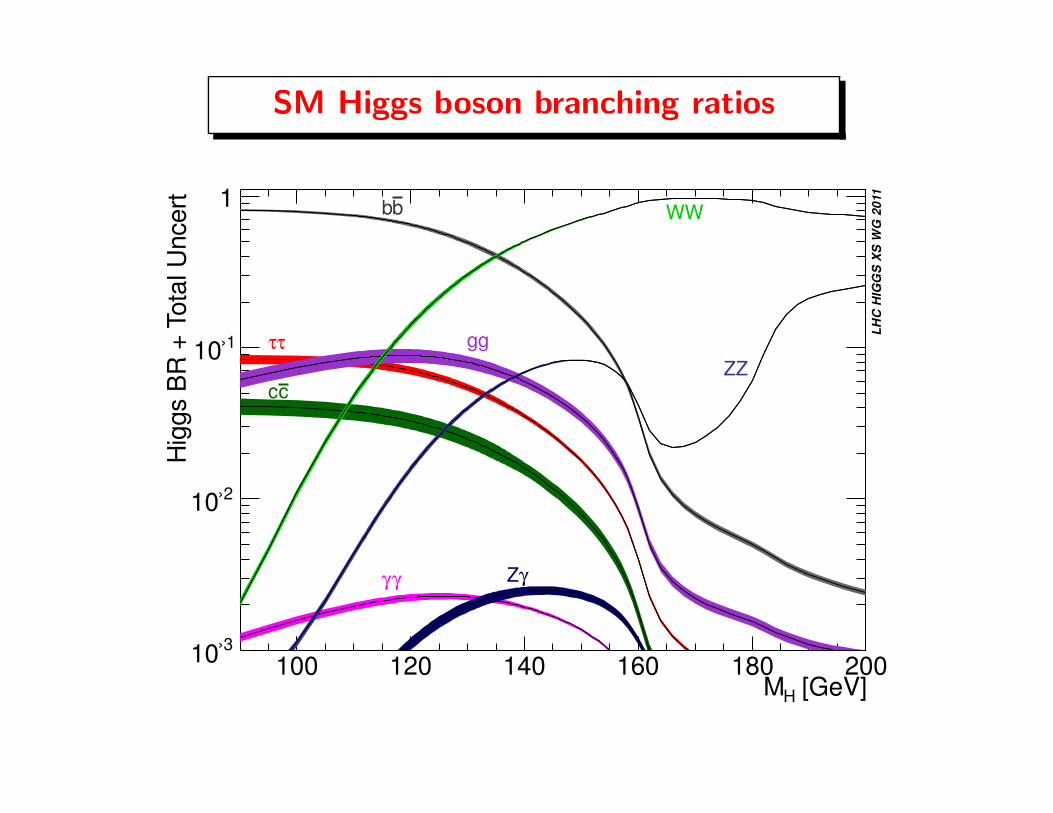
SM Higgs boson branching ratios

[GeV]HM100 120 140 160 180 200

Hig

gs B

R +

Tota

l U

ncert

›310

›210

›110

1

LH

C H

IGG

S X

S W

G 2

011

bb

ττ

cc

gg

γγ γZ

WW

ZZ

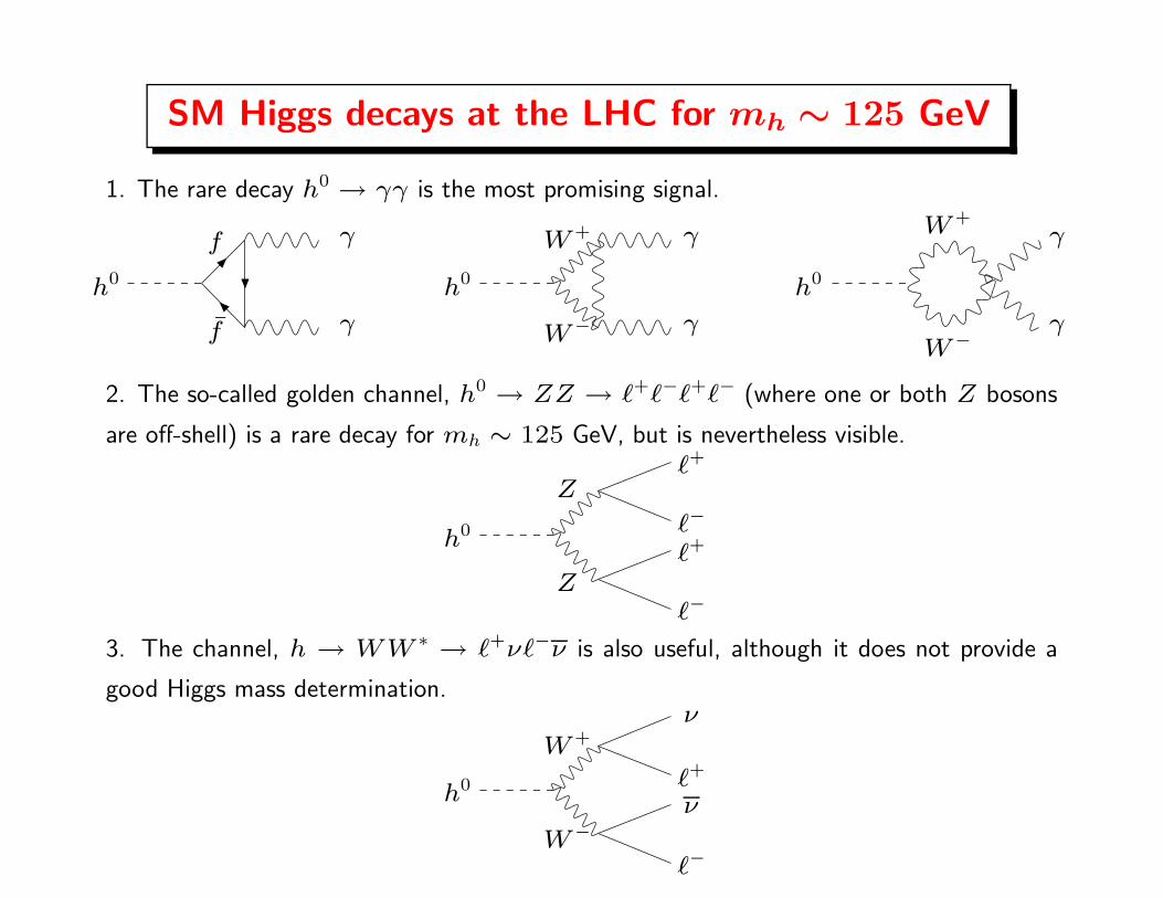
SM Higgs decays at the LHC for mh ∼ 125 GeV

1. The rare decay h0 → γγ is the most promising signal.

h0

γ

γ

f

f

h0

γ

γ

W +

W−

h0

γ

γ

W +

W−

2. The so-called golden channel, h0 → ZZ → `+`−`+`− (where one or both Z bosons

are off-shell) is a rare decay for mh ∼ 125 GeV, but is nevertheless visible.

h0

`+

`−

`+

`−

Z

Z

3. The channel, h → WW ∗ → `+ν`−ν is also useful, although it does not provide a

good Higgs mass determination.

h0

ν

`+

ν

`−

W +

W−

The LHC Discovery of 4 July 2012

The CERN update of the search for the SM Higgs boson, simulcast at ICHEP-2012 in Melbourne, Australia

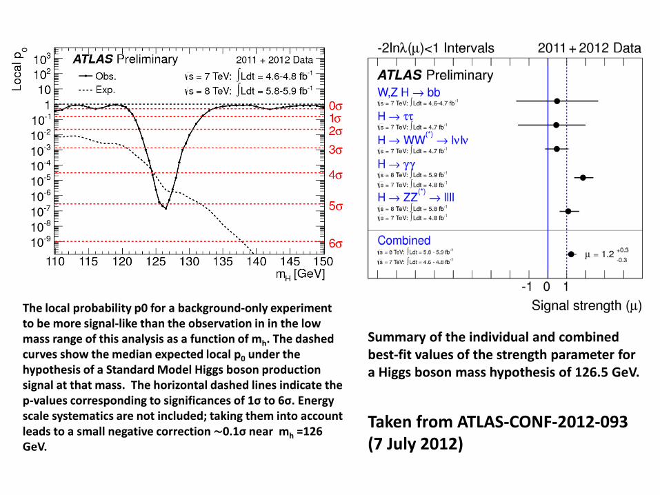
The local probability p0 for a background-only experiment to be more signal-like than the observation in in the low mass range of this analysis as a function of mh. The dashed curves show the median expected local p0 under the hypothesis of a Standard Model Higgs boson production signal at that mass. The horizontal dashed lines indicate the p-values corresponding to significances of 1σ to 6σ. Energy scale systematics are not included; taking them into account leads to a small negative correction ∼0.1σ near mh =126 GeV.

Summary of the individual and combined best-fit values of the strength parameter for a Higgs boson mass hypothesis of 126.5 GeV.

Taken from ATLAS-CONF-2012-093 (7 July 2012)

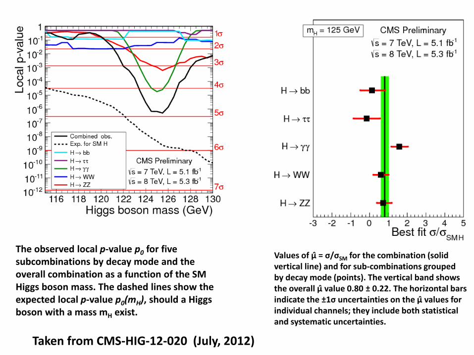
The observed local p-value p0 for five subcombinations by decay mode and the overall combination as a function of the SM Higgs boson mass. The dashed lines show the expected local p-value p0(mH), should a Higgs boson with a mass mH exist.

Values of μ = σ/σSM for the combination (solid vertical line) and for sub-combinations grouped by decay mode (points). The vertical band shows the overall μ value 0.80 ± 0.22. The horizontal bars indicate the ±1σ uncertainties on the μ values for individual channels; they include both statistical and systematic uncertainties.

Taken from CMS-HIG-12-020 (July, 2012)

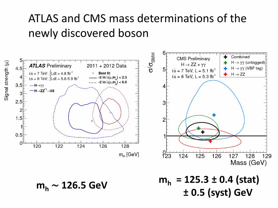
ATLAS and CMS mass determinations of the newly discovered boson

mh ∼ 126.5 GeV mh = 125.3 ± 0.4 (stat) ± 0.5 (syst) GeV

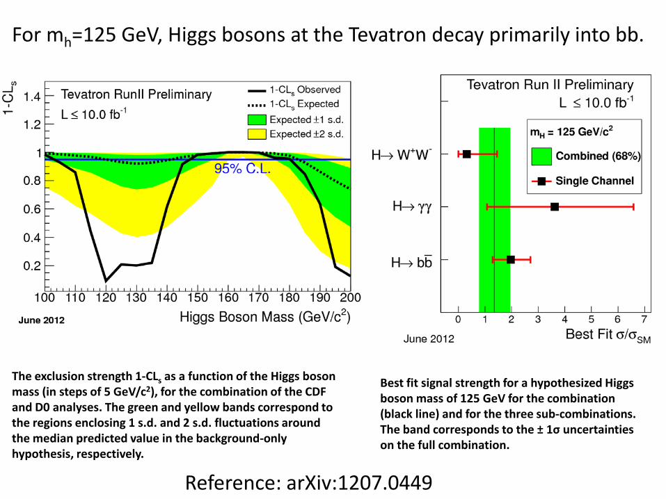
Best fit signal strength for a hypothesized Higgs boson mass of 125 GeV for the combination (black line) and for the three sub-combinations. The band corresponds to the ± 1σ uncertainties on the full combination.

Reference: arXiv:1207.0449

For mh=125 GeV, Higgs bosons at the Tevatron decay primarily into bb.

The exclusion strength 1-CLs as a function of the Higgs boson mass (in steps of 5 GeV/c2), for the combination of the CDF and D0 analyses. The green and yellow bands correspond to the regions enclosing 1 s.d. and 2 s.d. fluctuations around the median predicted value in the background-only hypothesis, respectively.

Hints of the Standard Model demise?

Suppose we accept the LHC observation of a new boson and identify it as

the SM Higgs boson. What does that imply for the Standard Model?

The Standard Model is an effective theory that provides an excellent

description of fundamental physics at the electroweak scale. We know that

the Standard Model must break down at the Planck scale, MPL ∼ 1019 GeV,

where the gravitational interactions can no longer be ignored. But, might

the Standard Model persist as a good effective field theory all the way up

to the Planck scale?

Note: Strictly speaking, neutrinos are massless in the Standard Model. One

elegant way to incorporate neutrino masses is the seesaw mechanism, which

introduces right handed neutrinos with Majorana masses of order 1014 GeV.

So, to be more precise, one can ask whether the seesaw-extended Standard

Model can persist all the way up to the Planck scale?

Electroweak symmetry breaking has something to say here. The EWSB

scalar dynamics of the Standard Model was previously analyzed at tree-

level. Do we really know that the minimum of the scalar potential is at

v = 246 GeV? What about potential minima at very large values of the

field, approaching the Planck scale. In this regime, a radiatively-corrected

scalar potential could include large logarithmic contributions, e.g. ln(Φ/v)

for large field values, that can spoil the perturbation analysis. However, such

large logarithms can be re-summed using renormalization group methods.

Without introducing the technical details, let me quote the final result. The

one-loop renormalization-group-improved scalar potential of the Standard

Model is give by

V (Φ) = µ2(t)G2(t)Φ†Φ + 12λ(t)G4(t)(Φ†Φ)2 ,

with t = ln(Φ2/M2) and M is the scale at which couplings are evaluated.

The running Higgs self-coupling evolves according to

dλ(t)

dt= βλ[gi(t), λ(t)] ,

where the gi include all relevant gauge and Yukawa couplings. The gi

also evolve with scale M according to their corresponding β-functions. The

evolution of µ2(t) can also be determined although it is not of much interest

to us here. Finally,

G(t) = exp

{

−∫ t

0

dt′ γ[gi(t′), λ(t′)

}

,

where γ is the anomalous dimensions of the scalar field. G(t) is necessarily

positive, but its precise value is not critical to this discussion.

It is convenient to fix M at the electroweak scale. Then, as Φ get large t

increases in value.

Let us return to

V (Φ) = µ2(t)G2(t)Φ†Φ + 12λ(t)G4(t)(Φ†Φ)2 ,

As t increases, if λ(t) is driven to infinity (say at one loop), we say we

have encountered a Landau pole. One should be a little careful as the

perturbative evolution of λ breaks down when λ becomes significantly larger

than 1. Nevertheless, there is good reason to suppose that the presence of

a Landau pole is an indication that the degrees of freedom of the effective

theory must be reorganized in some way. The Standard Model does not

provide a good description of the physics above this energy scale.

Suppose λ(t) is driven negative at some scale. In this case, the minimum of

the scalar potential at v = 246 GeV is no longer a global minimum. Indeed,

there is the potential for compete instability unless the potential turns

around again at an even higher energy scale. Presumably, this instability

is also an indication that the Standard Model does not provide a good

description of the physics above this energy scale.

Since m2h = λv2, where λ is evaluated at the scale of electroweak symmetry

breaking, the value of the Higgs mass provides the low energy boundary

condition for the evolution of λ at higher energy scales. Thus, the value of

the Higgs mass provides information of the possible demise of the Standard

Model at higher energies.

At one-loop, the behavior of λ(t) is controlled primarily by:

dλ

dt=

3

16π2

{

2λ2 + 2λh2t − 2h4

t − 12λ(3g2 + g′ 2) + 1

8

[

2g4 + (g2 + g′ 2)2]

}

dht

dt=

1

16π2

[

94h

3t − 4g2

sht − 98g

2ht − 1724g

′ 2ht

]

,

dg2s

dt= − 7g4

s

16π2,

where λ(0) = m2h/v and ht(0) =

√2mt/v and the low-energy values of the

gauge couplings set the boundary conditions.

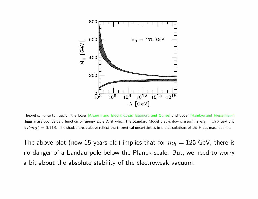
Theoretical uncertainties on the lower [Altarelli and Isidori; Casas, Espinosa and Quiros] and upper [Hambye and Riesselmann]

Higgs mass bounds as a function of energy scale Λ at which the Standard Model breaks down, assuming mt = 175 GeV and

αs(mZ) = 0.118. The shaded areas above reflect the theoretical uncertainties in the calculations of the Higgs mass bounds.

The above plot (now 15 years old) implies that for mh = 125 GeV, there is

no danger of a Landau pole below the Planck scale. But, we need to worry

a bit about the absolute stability of the electroweak vacuum.

Some would argue that we may not have too worry too much if λ(t) is

driven negative at some large energy scale below the Planck scale. Even

if the electroweak vacuum is not absolutely stable (assuming that the true

minimum lies at very large field values), all we should really impose is that

the electroweak vacuum, if metastable, should have a lifetime much longer

than the age of the universe. The latter condition would be satisfied if

mh = 125 GeV.

If one prefers to impose absolute stability of the SM Higgs potential, then

recent updated two-loop studies suggest that the SM must break down

below the Planck scale. To quote from G. Degrassi et al., arXiv:1205.6497,

“While [the Higgs self-coupling parameter evaluated] at the Planck

scale is remarkably close to zero, absolute stability of the Higgs

potential is excluded at 98% CL for mh < 126 GeV.”

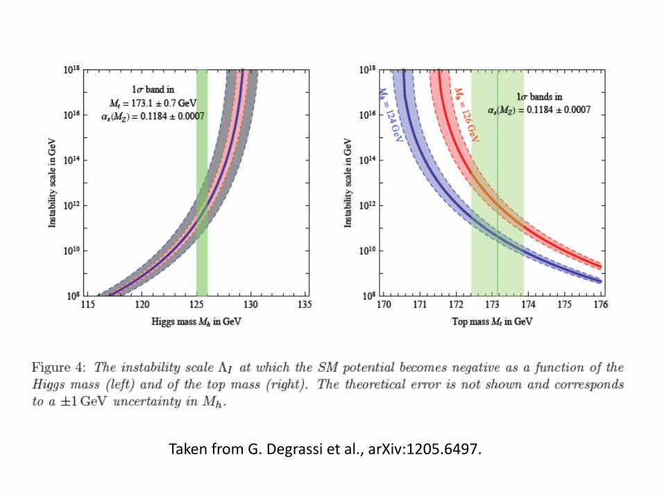
Taken from G. Degrassi et al., arXiv:1205.6497.

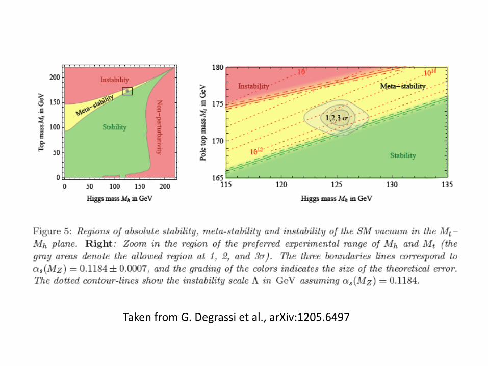
Taken from G. Degrassi et al., arXiv:1205.6497

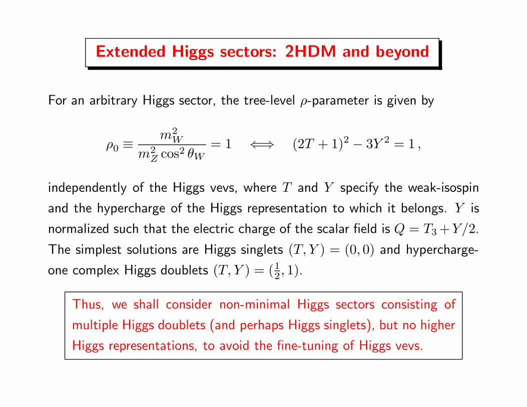
Extended Higgs sectors: 2HDM and beyond

For an arbitrary Higgs sector, the tree-level ρ-parameter is given by

ρ0 ≡ m2W

m2Z cos2 θW

= 1 ⇐⇒ (2T + 1)2 − 3Y 2 = 1 ,

independently of the Higgs vevs, where T and Y specify the weak-isospin

and the hypercharge of the Higgs representation to which it belongs. Y is

normalized such that the electric charge of the scalar field is Q = T3 +Y/2.

The simplest solutions are Higgs singlets (T, Y ) = (0, 0) and hypercharge-

one complex Higgs doublets (T, Y ) = (12, 1).

Thus, we shall consider non-minimal Higgs sectors consisting of

multiple Higgs doublets (and perhaps Higgs singlets), but no higher

Higgs representations, to avoid the fine-tuning of Higgs vevs.

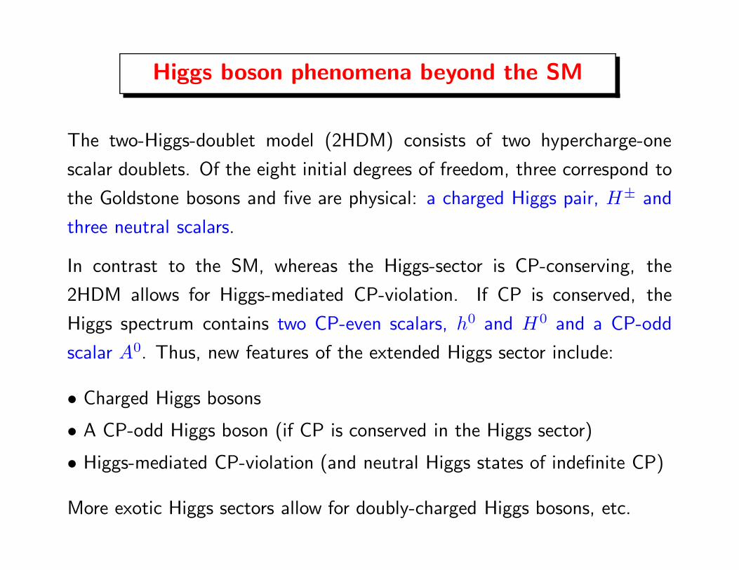
Higgs boson phenomena beyond the SM

The two-Higgs-doublet model (2HDM) consists of two hypercharge-one

scalar doublets. Of the eight initial degrees of freedom, three correspond to

the Goldstone bosons and five are physical: a charged Higgs pair, H± and

three neutral scalars.

In contrast to the SM, whereas the Higgs-sector is CP-conserving, the

2HDM allows for Higgs-mediated CP-violation. If CP is conserved, the

Higgs spectrum contains two CP-even scalars, h0 and H0 and a CP-odd

scalar A0. Thus, new features of the extended Higgs sector include:

• Charged Higgs bosons

• A CP-odd Higgs boson (if CP is conserved in the Higgs sector)

• Higgs-mediated CP-violation (and neutral Higgs states of indefinite CP)

More exotic Higgs sectors allow for doubly-charged Higgs bosons, etc.

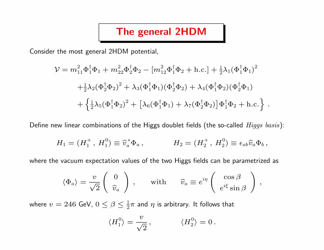
The general 2HDM

Consider the most general 2HDM potential,

V = m211Φ

†1Φ1 + m2

22Φ†2Φ2 − [m2

12Φ†1Φ2 + h.c.] + 1

2λ1(Φ†1Φ1)

2

+12λ2(Φ

†2Φ2)

2+ λ3(Φ

†1Φ1)(Φ

†2Φ2) + λ4(Φ

†1Φ2)(Φ

†2Φ1)

+n

12λ5(Φ

†1Φ2)

2 +ˆλ6(Φ

†1Φ1) + λ7(Φ

†2Φ2)

˜Φ†

1Φ2 + h.c.o

.

Define new linear combinations of the Higgs doublet fields (the so-called Higgs basis):

H1 = (H+1 , H

01) ≡ bv ∗

a Φa , H2 = (H+2 , H

02) ≡ εabbvaΦb ,

where the vacuum expectation values of the two Higgs fields can be parametrized as

〈Φa〉 =v√2

0

bva

!, with bva ≡ eiη

cos β

eiξ sin β

!,

where v = 246 GeV, 0 ≤ β ≤ 12π and η is arbitrary. It follows that

〈H01〉 =

v√2

, 〈H02〉 = 0 .

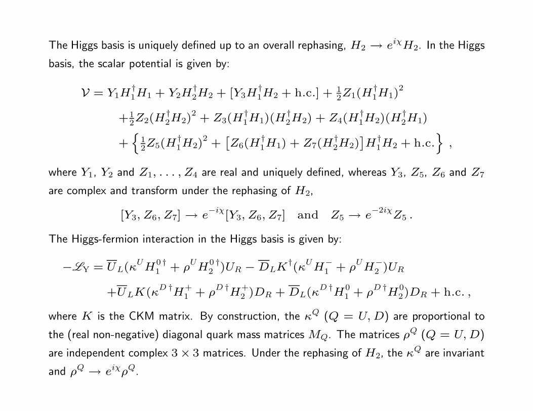
The Higgs basis is uniquely defined up to an overall rephasing, H2 → eiχH2. In the Higgs

basis, the scalar potential is given by:

V = Y1H†1H1 + Y2H

†2H2 + [Y3H

†1H2 + h.c.] + 1

2Z1(H†1H1)

2

+12Z2(H

†2H2)

2 + Z3(H†1H1)(H

†2H2) + Z4(H

†1H2)(H

†2H1)

+n

12Z5(H

†1H2)

2 +ˆZ6(H

†1H1) + Z7(H

†2H2)

˜H†

1H2 + h.c.o

,

where Y1, Y2 and Z1, . . . , Z4 are real and uniquely defined, whereas Y3, Z5, Z6 and Z7

are complex and transform under the rephasing of H2,

[Y3, Z6, Z7] → e−iχ

[Y3, Z6, Z7] and Z5 → e−2iχ

Z5 .

The Higgs-fermion interaction in the Higgs basis is given by:

−LY = UL(κUH0 †1 + ρUH0 †

2 )UR − DLK†(κUH−1 + ρUH−

2 )UR

+ULK(κD †H+1 + ρD †H+

2 )DR + DL(κD †H01 + ρD †H0

2)DR + h.c. ,

where K is the CKM matrix. By construction, the κQ (Q = U, D) are proportional to

the (real non-negative) diagonal quark mass matrices MQ. The matrices ρQ (Q = U, D)

are independent complex 3× 3 matrices. Under the rephasing of H2, the κQ are invariant

and ρQ → eiχρQ.

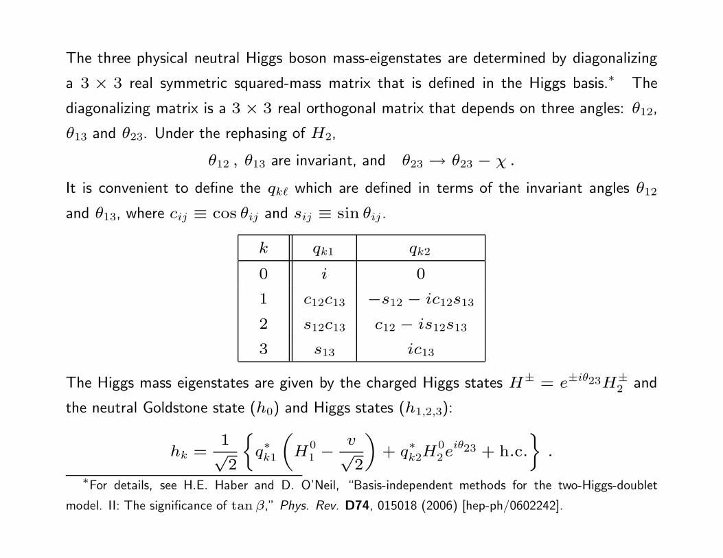
The three physical neutral Higgs boson mass-eigenstates are determined by diagonalizing

a 3 × 3 real symmetric squared-mass matrix that is defined in the Higgs basis.∗ The

diagonalizing matrix is a 3 × 3 real orthogonal matrix that depends on three angles: θ12,

θ13 and θ23. Under the rephasing of H2,

θ12 , θ13 are invariant, and θ23 → θ23 − χ .

It is convenient to define the qk` which are defined in terms of the invariant angles θ12

and θ13, where cij ≡ cos θij and sij ≡ sin θij .

k qk1 qk2

0 i 0

1 c12c13 −s12 − ic12s13

2 s12c13 c12 − is12s13

3 s13 ic13

The Higgs mass eigenstates are given by the charged Higgs states H± = e±iθ23H±2 and

the neutral Goldstone state (h0) and Higgs states (h1,2,3):

hk =1√2

q∗

k1

„H0

1 − v√2

«+ q∗

k2H02eiθ23 + h.c.

ff.

∗For details, see H.E. Haber and D. O’Neil, “Basis-independent methods for the two-Higgs-doublet

model. II: The significance of tan β,” Phys. Rev. D74, 015018 (2006) [hep-ph/0602242].

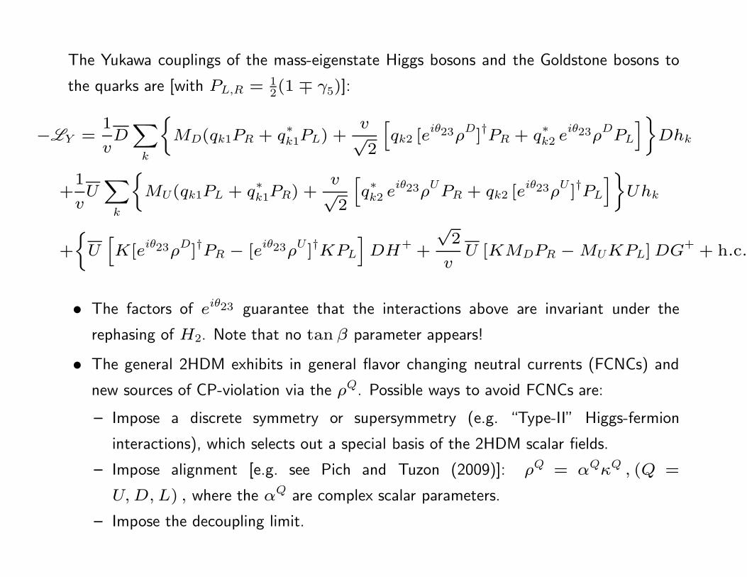
The Yukawa couplings of the mass-eigenstate Higgs bosons and the Goldstone bosons to

the quarks are [with PL,R = 12(1 ∓ γ5)]:

−LY =1

vDX

k

MD(qk1PR + q

∗k1PL) +

v√2

hqk2 [e

iθ23ρD]†PR + q

∗k2 e

iθ23ρD

PL

iffDhk

+1

vUX

k

MU(qk1PL + q∗

k1PR) +v√2

hq∗

k2 eiθ23ρUPR + qk2 [eiθ23ρU ]†PL

iffUhk

+

UhK[eiθ23ρD]†PR − [eiθ23ρU]†KPL

iDH+ +

√2

vU [KMDPR − MUKPL] DG+ + h.c.

ff

• The factors of eiθ23 guarantee that the interactions above are invariant under the

rephasing of H2. Note that no tan β parameter appears!

• The general 2HDM exhibits in general flavor changing neutral currents (FCNCs) and

new sources of CP-violation via the ρQ. Possible ways to avoid FCNCs are:

– Impose a discrete symmetry or supersymmetry (e.g. “Type-II” Higgs-fermion

interactions), which selects out a special basis of the 2HDM scalar fields.

– Impose alignment [e.g. see Pich and Tuzon (2009)]: ρQ = αQκQ , (Q =

U, D, L) , where the αQ are complex scalar parameters.

– Impose the decoupling limit.

The decoupling limit in the general 2HDM

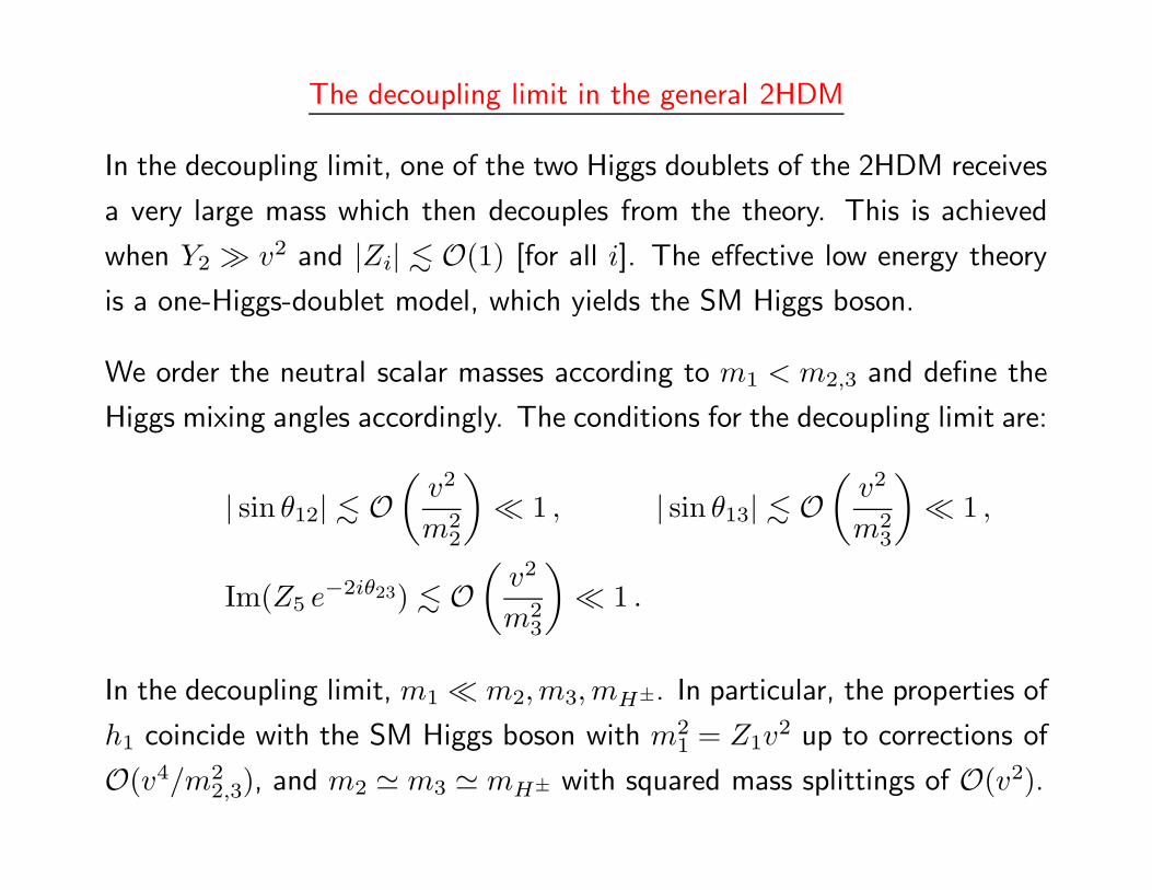
In the decoupling limit, one of the two Higgs doublets of the 2HDM receives

a very large mass which then decouples from the theory. This is achieved

when Y2 � v2 and |Zi| <∼ O(1) [for all i]. The effective low energy theory

is a one-Higgs-doublet model, which yields the SM Higgs boson.

We order the neutral scalar masses according to m1 < m2,3 and define the

Higgs mixing angles accordingly. The conditions for the decoupling limit are:

| sin θ12| <∼ O(

v2

m22

)

� 1 , | sin θ13| <∼ O(

v2

m23

)

� 1 ,

Im(Z5 e−2iθ23) <∼ O(

v2

m23

)

� 1 .

In the decoupling limit, m1 � m2,m3, mH±. In particular, the properties of

h1 coincide with the SM Higgs boson with m21 = Z1v

2 up to corrections of

O(v4/m22,3), and m2 ' m3 ' mH± with squared mass splittings of O(v2).

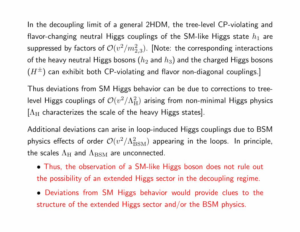
In the decoupling limit of a general 2HDM, the tree-level CP-violating and

flavor-changing neutral Higgs couplings of the SM-like Higgs state h1 are

suppressed by factors of O(v2/m22,3). [Note: the corresponding interactions

of the heavy neutral Higgs bosons (h2 and h3) and the charged Higgs bosons

(H±) can exhibit both CP-violating and flavor non-diagonal couplings.]

Thus deviations from SM Higgs behavior can be due to corrections to tree-

level Higgs couplings of O(v2/Λ2H) arising from non-minimal Higgs physics

[ΛH characterizes the scale of the heavy Higgs states].

Additional deviations can arise in loop-induced Higgs couplings due to BSM

physics effects of order O(v2/Λ2BSM) appearing in the loops. In principle,

the scales ΛH and ΛBSM are unconnected.

• Thus, the observation of a SM-like Higgs boson does not rule out

the possibility of an extended Higgs sector in the decoupling regime.

• Deviations from SM Higgs behavior would provide clues to the

structure of the extended Higgs sector and/or the BSM physics.

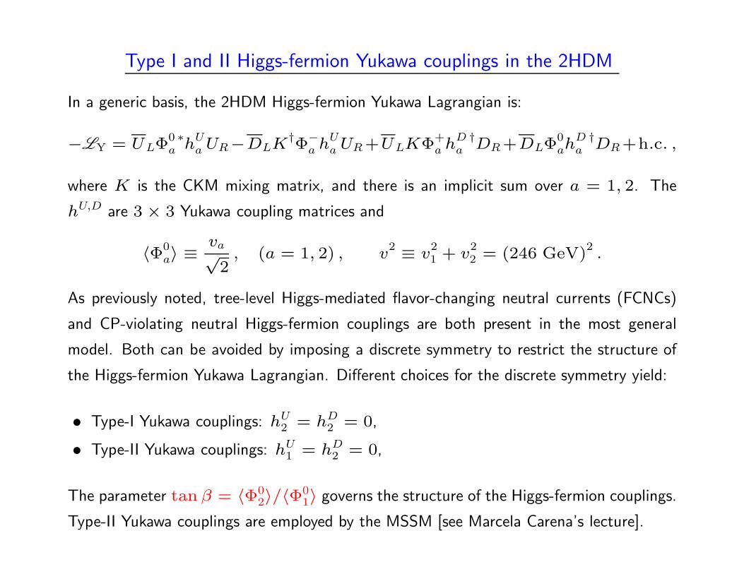
Type I and II Higgs-fermion Yukawa couplings in the 2HDM

In a generic basis, the 2HDM Higgs-fermion Yukawa Lagrangian is:

−LY = ULΦ0 ∗a hU

a UR−DLK†Φ−a hU

a UR+ULKΦ+a hD †

a DR+DLΦ0ah

D †a DR+h.c. ,

where K is the CKM mixing matrix, and there is an implicit sum over a = 1, 2. The

hU,D are 3 × 3 Yukawa coupling matrices and

〈Φ0a〉 ≡ va√

2, (a = 1, 2) , v

2 ≡ v21 + v

22 = (246 GeV)

2.

As previously noted, tree-level Higgs-mediated flavor-changing neutral currents (FCNCs)

and CP-violating neutral Higgs-fermion couplings are both present in the most general

model. Both can be avoided by imposing a discrete symmetry to restrict the structure of

the Higgs-fermion Yukawa Lagrangian. Different choices for the discrete symmetry yield:

• Type-I Yukawa couplings: hU2 = hD

2 = 0,

• Type-II Yukawa couplings: hU1 = hD

2 = 0,

The parameter tan β = 〈Φ02〉/〈Φ0

1〉 governs the structure of the Higgs-fermion couplings.

Type-II Yukawa couplings are employed by the MSSM [see Marcela Carena’s lecture].

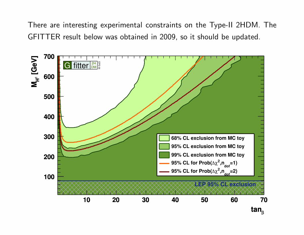
There are interesting experimental constraints on the Type-II 2HDM. The

GFITTER result below was obtained in 2009, so it should be updated.

βtan

10 20 30 40 50 60 70

[G

eV

]±

HM

100

200

300

400

500

600

700

LEP 95% CL exclusion

68% CL exclusion from MC toy

95% CL exclusion from MC toy

99% CL exclusion from MC toy

=1)dof

,n2χ∆95% CL for Prob(

=2)dof

,n2χ∆95% CL for Prob(

βtan

10 20 30 40 50 60 70

[G

eV

]±

HM

100

200

300

400

500

600

700

G fitter DM

2H

EP

S 0

9

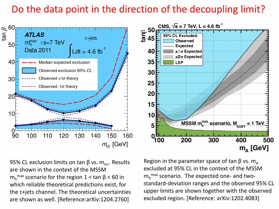
Region in the parameter space of tan β vs. mA excluded at 95% CL in the context of the MSSM mh

max scenario. The expected one- and two- standard-deviation ranges and the observed 95% CL upper limits are shown together with the observed excluded region. [Reference: arXiv:1202.4083]

95% CL exclusion limits on tan β vs. mH+. Results are shown in the context of the MSSM mh

max scenario for the region 1 < tan β < 60 in which reliable theoretical predictions exist, for the τ+jets channel. The theoretical uncertainties are shown as well. [Reference:arXiv:1204.2760]

Do the data point in the direction of the decoupling limit?

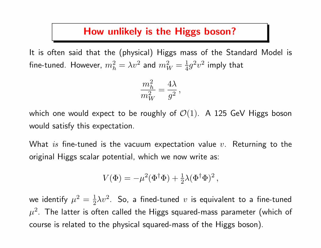
How unlikely is the Higgs boson?

It is often said that the (physical) Higgs mass of the Standard Model is

fine-tuned. However, m2h = λv2 and m2

W = 14g

2v2 imply that

m2h

m2W

=4λ

g2,

which one would expect to be roughly of O(1). A 125 GeV Higgs boson

would satisfy this expectation.

What is fine-tuned is the vacuum expectation value v. Returning to the

original Higgs scalar potential, which we now write as:

V (Φ) = −µ2(Φ†Φ) + 12λ(Φ†Φ)2 ,

we identify µ2 = 12λv2. So, a fined-tuned v is equivalent to a fine-tuned

µ2. The latter is often called the Higgs squared-mass parameter (which of

course is related to the physical squared-mass of the Higgs boson).

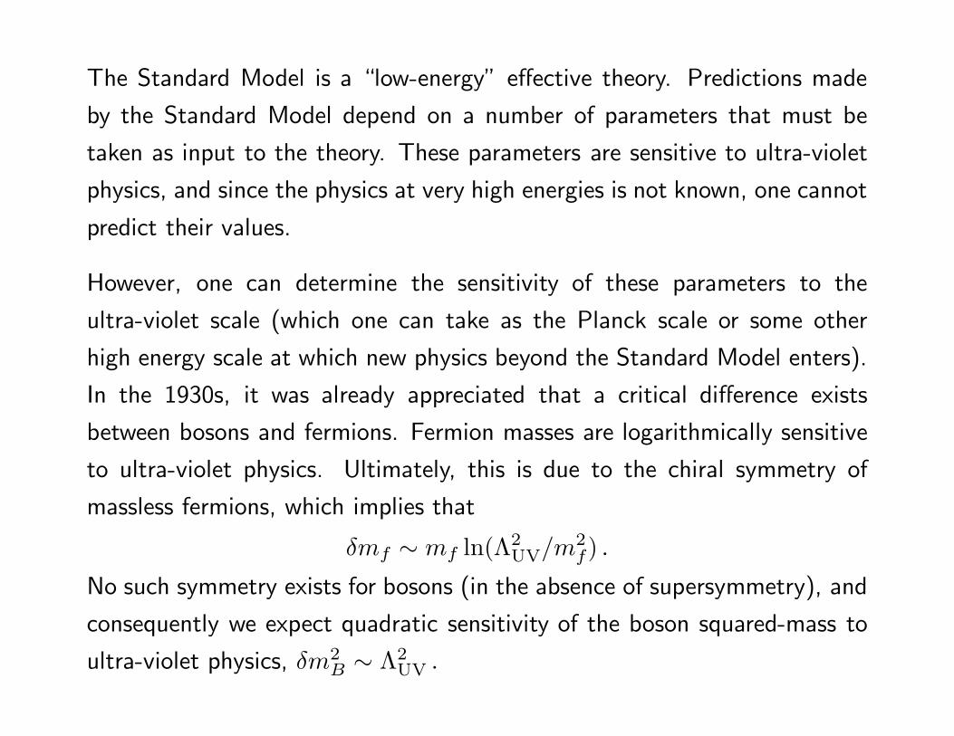
The Standard Model is a “low-energy” effective theory. Predictions made

by the Standard Model depend on a number of parameters that must be

taken as input to the theory. These parameters are sensitive to ultra-violet

physics, and since the physics at very high energies is not known, one cannot

predict their values.

However, one can determine the sensitivity of these parameters to the

ultra-violet scale (which one can take as the Planck scale or some other

high energy scale at which new physics beyond the Standard Model enters).

In the 1930s, it was already appreciated that a critical difference exists

between bosons and fermions. Fermion masses are logarithmically sensitive

to ultra-violet physics. Ultimately, this is due to the chiral symmetry of

massless fermions, which implies that

δmf ∼ mf ln(Λ2UV/m2

f) .

No such symmetry exists for bosons (in the absence of supersymmetry), and

consequently we expect quadratic sensitivity of the boson squared-mass to

ultra-violet physics, δm2B ∼ Λ2

UV .

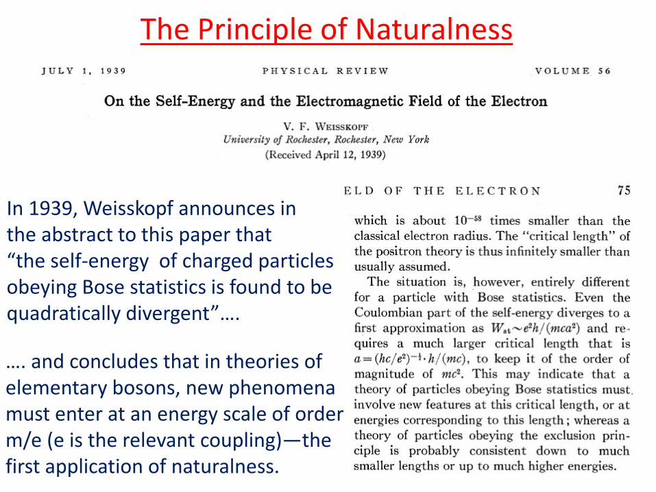
The Principle of Naturalness

In 1939, Weisskopf announces in the abstract to this paper that “the self-energy of charged particles obeying Bose statistics is found to be quadratically divergent”….

…. and concludes that in theories of elementary bosons, new phenomena must enter at an energy scale of order m/e (e is the relevant coupling)—the first application of naturalness.

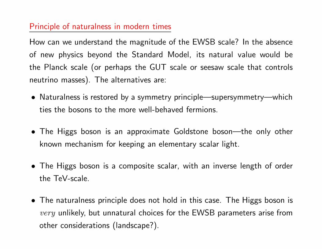
Principle of naturalness in modern times

How can we understand the magnitude of the EWSB scale? In the absence

of new physics beyond the Standard Model, its natural value would be

the Planck scale (or perhaps the GUT scale or seesaw scale that controls

neutrino masses). The alternatives are:

• Naturalness is restored by a symmetry principle—supersymmetry—which

ties the bosons to the more well-behaved fermions.

• The Higgs boson is an approximate Goldstone boson—the only other

known mechanism for keeping an elementary scalar light.

• The Higgs boson is a composite scalar, with an inverse length of order

the TeV-scale.

• The naturalness principle does not hold in this case. The Higgs boson is

very unlikely, but unnatural choices for the EWSB parameters arise from

other considerations (landscape?).

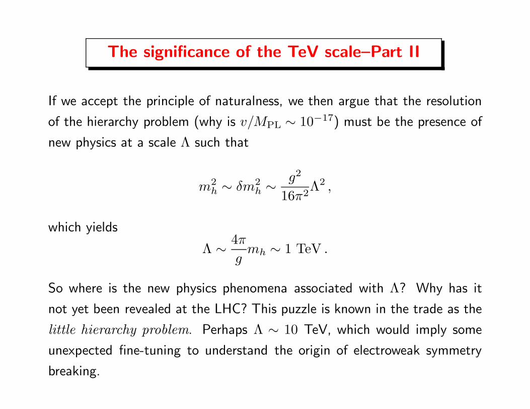
The significance of the TeV scale–Part II

If we accept the principle of naturalness, we then argue that the resolution

of the hierarchy problem (why is v/MPL ∼ 10−17) must be the presence of

new physics at a scale Λ such that

m2h ∼ δm2

h ∼ g2

16π2Λ2 ,

which yields

Λ ∼ 4π

gmh ∼ 1 TeV .

So where is the new physics phenomena associated with Λ? Why has it

not yet been revealed at the LHC? This puzzle is known in the trade as the

little hierarchy problem. Perhaps Λ ∼ 10 TeV, which would imply some

unexpected fine-tuning to understand the origin of electroweak symmetry

breaking.

All models of new physics beyond the Standard Model (BSM) are feeling

the tension of the little hierarchy. Nevertheless, proponents of naturalness

are still convinced that BSM physics will eventually be found at the LHC,

and the ultimate nature of the new physics will have profound implications

for the origin of EWSB.

It is interesting that the tension of the little hierarchy is felt in different ways

depending on the nature of the BSM physics. For example, compare the

significance of the Higgs mass in the MSSM as compared with a composite

Higgs model, where the Higgs boson is a pseudo-Goldstone boson (thanks

to Alex Pomarol for this comparison).

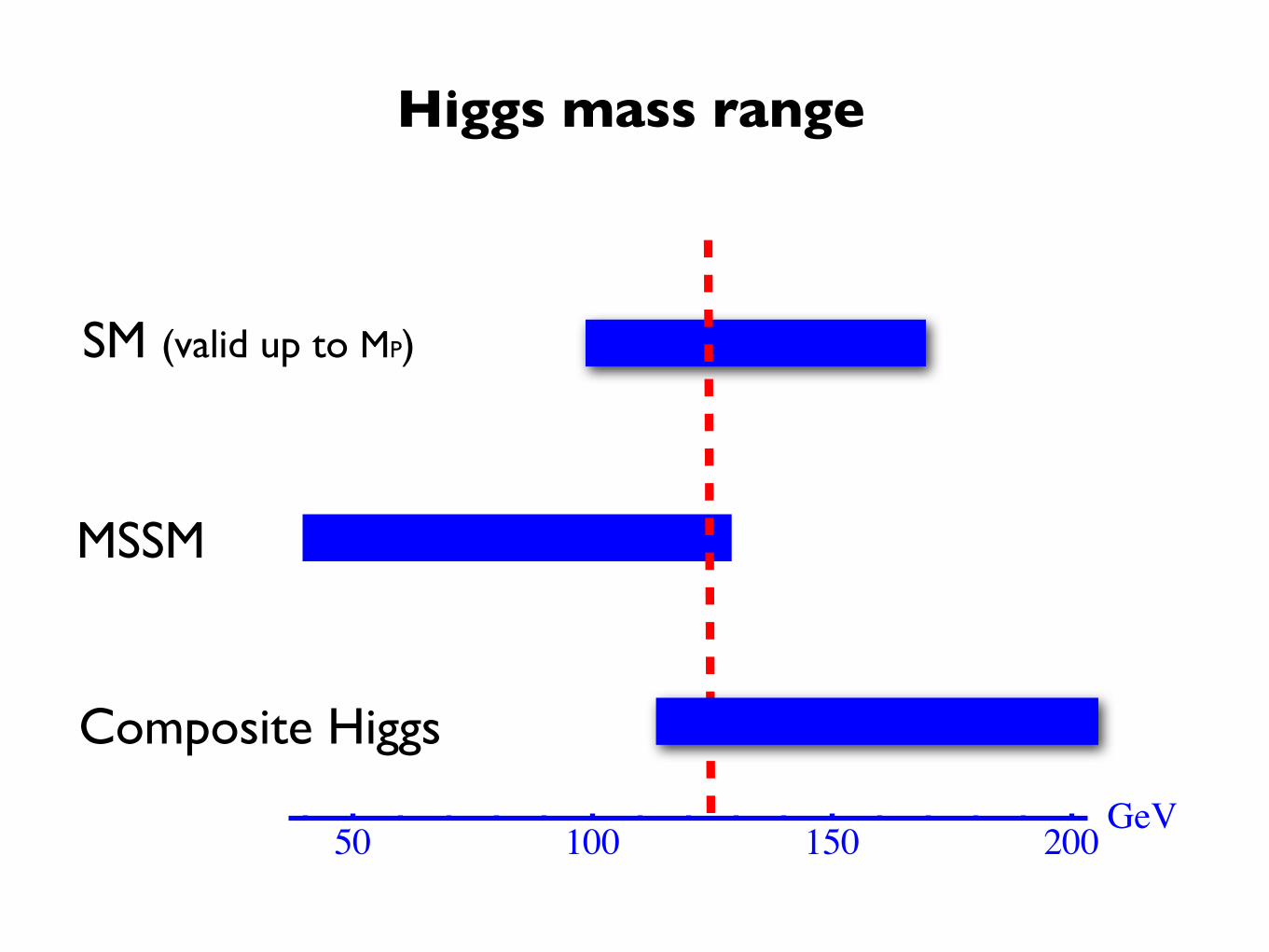
Higgs mass range

MSSM

SM (valid up to MP)

Composite Higgs

50 100 150 200GeV

The key questions looking forward

• Does the new boson discovered at the LHC exhibit the expected properties

of the SM Higgs boson (spin? parity? couplings?)

• Will further study of the properties of this new state yield significant

deviations from the SM Higgs boson expectations?

• How accurately can one measure the Higgs properties at the LHC? Do

we need a dedicated precision Higgs factory?

• Will new BSM physics be discovered at the LHC that will shed light on

the origin of EWSB?

These are exciting times. The July 4 discovery is not the end of the

Standard Model but the beginning of an exploration that will yield profound

insights into the theory of the fundamental particles and their interactions.