Econ 514: Probability and Statistics

Lecture 2: Random Variables and Expectation

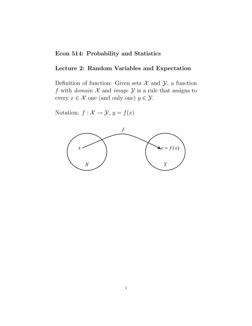
Definition of function: Given sets X and Y , a functionf with domain X and image Y is a rule that assigns toevery x ∈ X one (and only one) y ∈ Y .

Notation: f : X → Y , y = f(x)

1

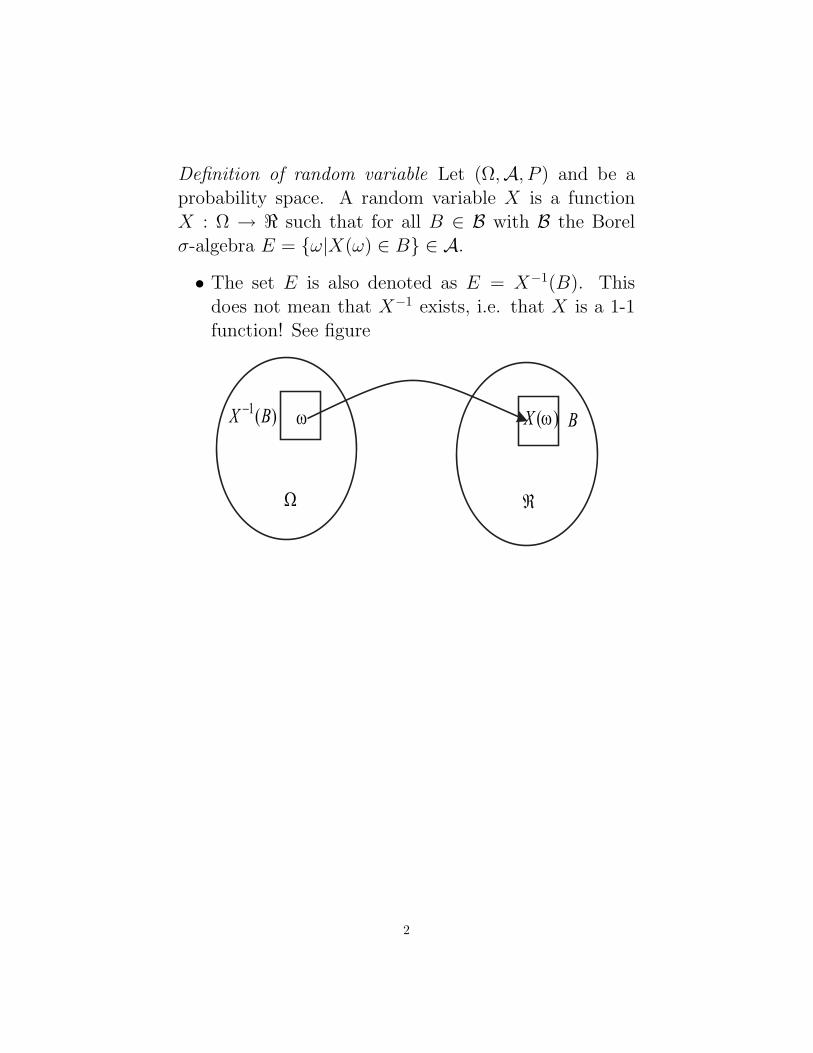
Definition of random variable Let (Ω,A, P ) and be aprobability space. A random variable X is a functionX : Ω → < such that for all B ∈ B with B the Borelσ-algebra E = ω|X(ω) ∈ B ∈ A.

• The set E is also denoted as E = X−1(B). Thisdoes not mean that X−1 exists, i.e. that X is a 1-1function! See figure

2

• A random variable X is a function that is in addi-tion Borel measurable. Why we need this will bediscussed later.

• Measurability is a more general concept. Becauserandom variables are always functions to < we needonly Borel measurability, because for < we alwaystake the Borel σ-algebra.

• Often the function X can take the values ∞ and−∞, i.e. X is a function the the extended real line< with the extended Borel σ-field B that contains allsets in B and the two points ∞,−∞.

Why random variables?

• Often outcomes of a random experiment are compli-cated.

• Random variable summarizes (aspects of) an out-come in a single number.

3

Example: Three tosses of a single coin.

• Outcome space

Ω = HHH, HHT, HTH, THH, HTT, THT,

TTH, TTT

• Define X ≡ number of H in 3 tosses

X(ω) = 3 if ω = HHH

= 2 if ω = HHT,HTH,THH

= 1 if ω = THT,TTH,HTT

= 0 if ω = TTT

• For some random experiment we can define manyrandom variables, e.g. in this example Y ≡ number of T before first H.

4

Measurability

• To establish measurability we use a generating classargument, because it is often easier to establish mea-surability on such a class.

• If E is a generating class for B, e.g. the intervals(−∞, x] or (x,∞), then we need only to show thatX−1(E) ∈ A for all E ∈ E .

Proof:

– Define C = B ∈ B|X−1(B) ∈ A. We show thatthis is a σ-field.

(i) ∅ ∈ C.

(ii) Note X−1(Bc) = X−1(B)c, because by defini-tion ω ∈ X−1(B)c iff X(ω) /∈ B iff X(ω) ∈ Bc.Hence X−1(Bc) ∈ A.

(iii) Note X−1(∪∞i=1Bi) = ∪∞i=1X−1(Bi), because

ω ∈ X−1(∪∞i=1Bi) iff X(ω) ∈ ∪∞i=1Bi. Hence,X−1(∪∞i=1Bi) ∈ A.

– Because C is a σ-field and E ⊆ C, we have B =σ(E) ⊆ C. Hence X−1(B) ∈ A for all B ∈ B, sothat X is Borel measurable.

5

Applications

• Let Ω = <, i.e. X : < → <. If X is a continuousfunction, then X is Borel measurable, because if E

is an open set (the open sets in < are a generatingclass), then X−1(E) is also open and hence in B.

• Let Xn, n = 1, 2, . . . be a sequence of random vari-ables, then Xsup = supn Xn and Xinf = infn Xn arealso random variables, i.e. they are Borel measur-able functions. Note that Xsup(ω) may be equal to∞ for some ω (and Xinf(ω) equal to −∞), i.e. theyare B measurable. To see this note that (x,∞) is agenerating class for B, and that

ω|Xsup(ω) > x = ∪nω|Xn(ω) > x

The last union is clearly in A. For Xinf take thegenerating sets (−∞, x).

• If limn→∞Xn = X exists (may be±∞), then this is arandom variable. To see this note that lim infn→∞Xn(ω) =supn infm≥n Xm(ω) and lim supn→∞Xn(ω) = infn supm≥n Xm(ω).From the previous result these are Borel measurablefunctions. We have

lim infn→∞

Xn(ω) ≤ X(ω) = limn→∞

Xn(ω) ≤ lim supn→∞

Xn(ω)

Hence if the limit exists, it is equal to the liminf andlimsup which are Borel measurable.

6

• Let X and Y be random variables, then Z = X + Y

is Borel measurable. Note that

A = ω|Z(ω) > z = ∪xω|X(ω) = x∩ω|Y (ω) > z−x

which involve an uncountable union. Because thecountable set of rational numbers is a dense subsetof <, for all ω with X(ω) > z − Y (ω) there is arational number r such that X(ω) > r > z − Y (ω).Hence

A = ∪rω|X(ω) > r ∩ ω|Y (ω) > z − r

which is a countable union.

7

We denote all Borel measurable functions X : Ω → <by M and the subset of Borel measurable nonnegativefunctions by M+. A special class of nonnegative Borelmeasurable functions are the simple functions that canbe written as

X(ω) =n∑i

αiIAi(ω)

with IA the indicator function of the event A and Ai ∈A, i = 1, . . . , n a partition of Ω and αi ≥ 0, i = 1, . . . , nconstants. Each function in M+ can be approximatedby and increasing sequence of simple functions.

Theorem 1 For each X in M+, the sequence of simplefunctions

Xn(ω) = 2−n4n∑i=1

IX≥ i2n

(ω)

is such that 0 ≤ X1(ω) ≤ X2(ω) ≤ . . . ≤ Xn(ω) andXn(ω) ↑ X(ω) for all ω ∈ Ω.

Proof: If X(ω) ≥ 2n , then Xn(ω) = 2n If k2−n ≤X(ω) < (k + 1)2−n for some k = 0, 1, . . . , 4n − 1, thenXn(ω) = k2−n. See the figure for a graph and the claimfollows.

8

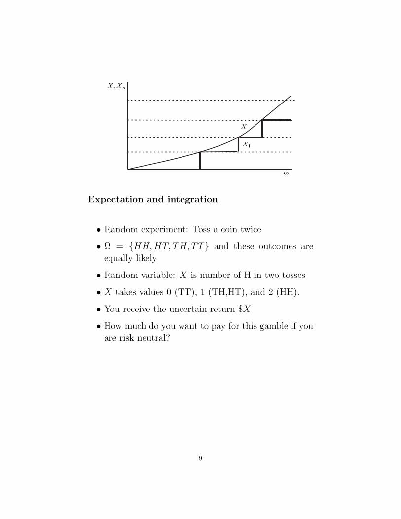
Expectation and integration

• Random experiment: Toss a coin twice

• Ω = HH,HT, TH, TT and these outcomes areequally likely

• Random variable: X is number of H in two tosses

• X takes values 0 (TT), 1 (TH,HT), and 2 (HH).

• You receive the uncertain return $X

• How much do you want to pay for this gamble if youare risk neutral?

9

Most people make the following computation:

• Consider a large number of repetitions of the randomexperiment.

• The relative frequency of values of X is 1/4 (X = 0),1/2 (X = 1), 1/4 (X = 2).

• On average (over the repetitions) X is

0.1

4+ 1.

1

2+ 2.

1

4= 1

• You are willing to pay $1 for the gamble. Call thisthe expected value of X, denoted by E(X).

Direct computation

• Note that X is a nonnegative simple function for thepartition A1 = TT, A2 = HT, TH, A3 = HHand X(ω) = 0.IA1

(ω) + 1.IA2(ω) + 2.IA3

(ω).

• E(X) = 0.P (A1) + 1.P (A2) + 2.P (A3) = 1.

• In general if X(ω) =∑n

i αiIAi(ω) is a simple func-

tion, the expected value of X is

E(X) =n∑

i=1

αiP (Ai)

• Note that this is a weighted average of the valuesof X, the weights being the probabilities of thesevalues.

• This suggests the notation

E(X) =

∫Ω

X(ω)dP (ω) =

∫XdP

10

How do you compute E(X) for a general random variableX? We use Theorem 1:

• Let X be a nonnegative random variable defined onthe probability space (Ω,A, P ).

• By Theorem 1 there is an increasing sequence of sim-ple functions Xn that has limit X. This is why weneed that X is Borel measurable to be able to defineE(X).

• Define for simple functions XS

E(X) =

∫XdP = sup

XS

E(XS)|X ≥ XS

Properties of E(X)

(i) E(IA) = P (A) for A ∈ A.

(ii) E(0) = 0 with 0 the null function that assigns 0 toall ω ∈ Ω.

11

(iii) For α, β ≥ 0 and nonnegative Borel measurable func-tions X, Y

E(αX + βY ) = αE(X) + βE(Y )

This is the linearity of the expectation.

Proof: Note that if XS, YS are simple functions thenso is ZS = XS + YS. Also E(ZS) = E(XS) + E(YS).

E(X)+E(Y ) = supXS

E(XS)|X ≥ XS+supYS

E(YS)|Y ≥ YS =

= supXS ,YS

E(XS) + E(YS)|X ≥ XS, Y ≥ YS ≤

≤ supXS ,YS

E(XS + YS)|X + Y ≥ XS + YS =

= supZS

E(ZS)|X + Y ≥ ZS = E(X + Y )

Next we prove E(X+Y ) ≤ E(X)+E(Y ). Let ZS bea simple function with ZS ≤ X+Y and let ε > 0. Weconstruct simple functions XS ≤ X and YS ≤ Y suchthat (1 − ε)ZS ≤ XS + YS. We do the constructionfor ZS = IA. The general case is analogous. Takeε = 1

m and denote lj = jm . Define

XS(ω) = IA(ω)

(IX≥1(ω) +

m∑j=1

lj−1Ilj−1≤X<lj(ω)

)

YS(ω) = IA(ω)m∑

j=1

(1− lj)Ilj−1≤X<lj(ω)

Obviously XS ≤ X. Now X(ω) + Y (ω) ≥ 1 for allω ∈ Ω. Hence for lj−1 ≤ X < lj, we have Y >

12

1− lj = YS. This holds for all j and hence YS ≤ Y .Finally, because 1− lj + lj−1 = 1− ε, we have

XS(ω) + YS(ω) =

= IA(ω)IX≥1(ω)+(1−ε)IA(ω)m∑

j=1

Ilj−1≤X<lj(ω) ≥ (1−ε)IA(ω)

Hence for all ZS ≤ X + Y

E(X) + E(Y ) ≥ E(XS) + E(YS) ≥ (1− ε)E(ZS)

and if we take the sup over all ZS ≤ X + Y , wefind E(X) + E(Y ) ≥ (1 − ε)E(X + Y ). Becauseε > 0 is arbitrary, this is still true if ε ↓ 0. Fromthe definition it follows directly that for all α ≥ 0,E(αX) = αE(X).

(iv) If X(ω) ≤ Y (ω) for all ω ∈ Ω, then E(X) ≤ E(Y ).

Proof: E(X) = E(Y )− E(Y −X) ≥ E(X)

13

(v) If Xn ↑ X is an increasing sequence of nonnegativeBorel measurable functions, then E(Xn) ↑ E(X).This is the monotone convergence property.

Proof: Let XS =∑m

i=1 αiIAibe a simple function

with X ≥ XS. Define the simple functions

XnS(ω) =m∑

i=1

(1− ε)αiIAi(ω)IXn≥(1−ε)αi

(ω)

Then XnS ≤ Xn and

E(Xn) ≥ E(XnS) = (1−ε)m∑

i=1

αiP (Ai∩ω|Xn(ω) ≥ (1−ε)αi)

Because Xn ↑ X ≥ αi for ω ∈ Ai, Ai ∩ ω|Xn(ω) ≥(1 − ε)αi ↑ Ai and hence P (Ai ∩ ω|Xn(ω) ≥ (1 −ε)αi) ↑ P (Ai). Hence for all XS ≤ X

limn→∞

E(Xn) ≥ (1− ε)E(XS)

Take the sup over all XS ≤ X and let ε ↓ 0 to obtain

limn→∞

E(Xn) ≥ E(X)

Because Xn ≤ X, also

limn→∞

E(Xn) ≤ E(X)

14

Extension to all random variables

• Until now E(X) only defined for nonnegative ran-dom variables.

• For arbitrary random variable X we can always write

X(ω) = X+(ω)−X−(ω)

with X+(ω) = maxX(ω), 0 and X−(ω) = −minX(ω), 0.Note X+, X− are nonnegative.

• We define

E(X) = E(X+)− E(X−) =

∫Ω

X+dP −∫

ΩX−dP

• This is well-defined unless E(X+) = E(X−) = ∞.To avoid this we can require E(X+) < ∞, E(X−) <

∞ or E(|X|) < ∞. A random variable X withE(|X|) < ∞ is called integrable.

• Application: Jensen’s inequality. A function f :< → < is convex if for all 0 < λ < 1, f(λx1 +(1− λ)x2) ≤ λf(x1) + (1− λ)f(x2). If f is convex

– E = x|f(x) ≤ t is a convex subset of < andhence an interval. Hence, f is Borel measurable.

Proof: x1, x2 ∈ E, then f(λx1 + (1 − λ)x2) ≤λf(x1) + (1− λ)f(x2) ≤ t.

– For all x, x0, f(x) ≥ f(x0) + α(x − x0) with α aconstant that may depend on x0.

15

• Note

f(x) ≥ f(x0)+α(x−x0) ≥ −|f(x0)|− |α|(|x|+ |x0|)

Hence E(f(X)−) < ∞ if X is integrable and E(f(X)is well-defined.

• Take x0 = E(X) to obtain

E(f(X)) ≥ f(E(X))+α(E(X)−E(X)) = f(E(X))

16

Lebesgue integrals

• The expectation of X is the integral of X w.r.t. tothe probability measure P .

• The same definition applies if P is replaced by a mea-sure µ, i.e. if the condition that µ(Ω) = 1 is droppedand replaced by µ(∅) = 0 (the other conditions re-main).

• Special case is Lebesgue measure, defined by m([a, b]) =b − a. This is the length of the interval. It impliesm((a, b)) = b−a (because the Lebesgue measure of apoint is 0) and because the open intervals are a gen-erating class the definition can be uniquely extendedto all sets in the Borel field B.

• The integral of Borel measurable f : < → < w.r.t.Lebesgue measure is denoted by

∫∞−∞ f(x)dx. The

notation is the same as the (improper) Riemann in-tegral of f .

• If f is integrable, i.e. if the Lebesgue integral∫∞−∞ |f(x)|dx <

∞, then the Lebesgue integral is equal to the Rie-mann integral if the latter exists. If

∫∞−∞ |f(x)|dx =

∞, the improper Riemann integral limt→∞∫ t

−t f(x)dx

may exist, while the Lebesgue integral is not defined.

• Except for this special case you can compute Lebesgueintegrals with all the calculus tricks.

• The theory of Lebesgue integration is easier thanthat of Riemann integration, in particular if order orintegration and limit or integration and differentia-tion has to be interchanged.

17

Integration and limits

• Often we have a sequence of random variables Xn, n =1, 2, . . . and we need to know limn→∞E(Xn) = limn→∞

∫XndP .

Can we interchange limit and integral?

• We want to take the derivative w.r.t. of E(f(X, t)) =inf f(X, t)dP . Can we interchange differentiationand integration?

What can go wrong:

• Consider the probability space [0, 1],B[0, 1], P ) withB[0, 1] the σ-field obtained by the intersections of thesets in B with [0, 1] and P ((a, b)) = b− a.

• Define the sequence Xn(ω) = n2I(0, 1n )(ω).

• Xn(ω) → 0 for all 0 ≤ ω ≤ 1, but E(Xn) = n →∞.

• limn→∞E(Xn) = ∞ 6= 0 = E(limn→∞Xn)

Theorem 2 (Fatou’s Lemma) Let Xn be a sequenceof nonnegative random variables (need not converge), then

E(lim infn→∞

Xn) ≤ lim infn→∞

E(Xn)

Proof: Remember lim infn→∞Xn = limn→∞ infm≥n Xm.Define Yn = infm≥nXm. We have for all n, Yn ≤ Xn.Moreover, Yn is an increasing sequence of nonnegativerandom variables, by monotone convergence E(lim infn→∞Xn) =limn→∞E(Yn). Finally, because E(Xn) ≤ E(Yn), wehave limn→∞E(Yn) ≤ lim infn→∞E(Xn).

18

Theorem 3 (Dominated convergence) Let Xn be asequence of integrable random variables and let the limitlimn→∞Xn(ω) = X(ω) exist for all ω ∈ Ω. If thereis a nonnegative integrable random variable Y such that|Xn(ω)| ≤ Y (ω) for all ω ∈ Ω and all n, then X isintegrable and limn→∞E(Xn) = E(X).

Proof: |X| ≤ Y and hence X is integrable. Consider thesequences Y +Xn and Y −Xn that are both nonnegativeand integrable. By Fatou’s lemma

E(Y +X) = E(lim infn→∞

(Y +Xn)) ≤ E(Y )+lim infn→∞

E(Xn)

E(Y −X) = E(lim infn→∞

(Y −Xn)) ≤ E(Y )−lim supn→∞

E(Xn)

because lim inf −Xn = − lim sup Xn. Cancel E(Y ) toobtain

lim supn→∞

E(Xn) ≤ E(X) ≤ lim infn→∞

E(Xn)

19

Application: Let f(X, t) be an integrable random vari-able for −δ < t < δ with δ > 0, let f(x, t) be differen-tiable in t on that interval and for all x. Consider thepartial derivative with respect to t and assume for all x

and −δ < t < δ ∣∣∣∣ ∂∂tf(x, t)

∣∣∣∣with M(X) an integrable random variable. Hence by themean value theorem∣∣∣∣f(x, t)− f(x, 0)

t

∣∣∣∣ ≤ ∣∣∣∣ ∂∂tf(x, t(x))

∣∣∣∣ ≤ M(x)

with t(x) = λ(x)t for some 0 ≤ λ(x) ≤ 1.Define the sequence of random variables

f(X, tn)− f(X, 0)

tn

with tn → 0. We have

limn→∞

E

(f(X, tn)− f(X, 0)

tn

)= lim

n→∞

E(f(X, tn))− E(f(X, 0))

tn

By dominated convergence we can interchange the limitand the expectation (integration), so that

E

(∂

∂tf(X, t)

)=

∂

∂tE(f(X, t))

20

Sets of measure 0

In integrals/expactations sets E ∈ A with P (E) = 0 canbe neglected.

Theorem 4 If the random variables X and Y are suchthat E = ω|X(ω) 6= Y (ω) with P (E) = 0, then E(X) =E(Y ).

Proof: If n is sufficiently large then X(ω) ≤ Y (ω) +n.IX 6=Y (ω). Because the sequence on the rhs is increas-ing, we have by monotone convergence

E(X) ≤ E(

limn→∞

(Y + n.IX 6=Y ))

= limn→∞

E(Y +n.IX 6=Y )) = E(Y )

Interchange X and Y to obtain, E(Y ) ≤ E(X).

21