1

8. One Function of Two Random Variables

Given two random variables X and Y and a function g(x,y),

we form a new random variable Z as

Given the joint p.d.f how does one obtain

the p.d.f of Z ? Problems of this type are of interest from a

practical standpoint. For example, a receiver output signal

usually consists of the desired signal buried in noise, and

the above formulation in that case reduces to Z = X + Y.

).,( YXgZ =

),,( yxf XY ),( zf Z

(8-1)

2

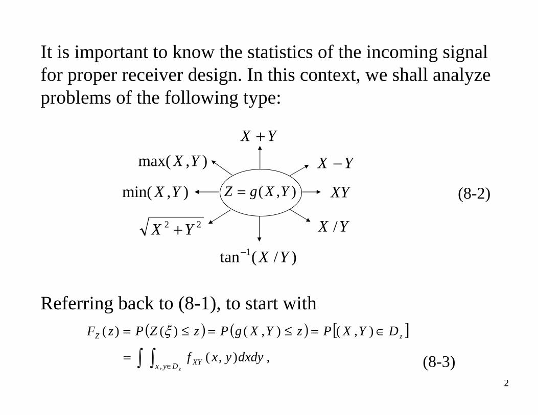
It is important to know the statistics of the incoming signal for proper receiver design. In this context, we shall analyze problems of the following type:

Referring back to (8-1), to start with

),( YXgZ =

YX +

)/(tan 1 YX−

YX −

XY

YX /

),max( YX

),min( YX

22 YX +

( ) ( ) [ ]

∫ ∫ ∈=

∈=≤=≤=

zDyx XY

zZ

dxdyyxf

DYXPzYXgPzZPzF

, ,),(

),(),()()( ξ

(8-2)

(8-3)

3

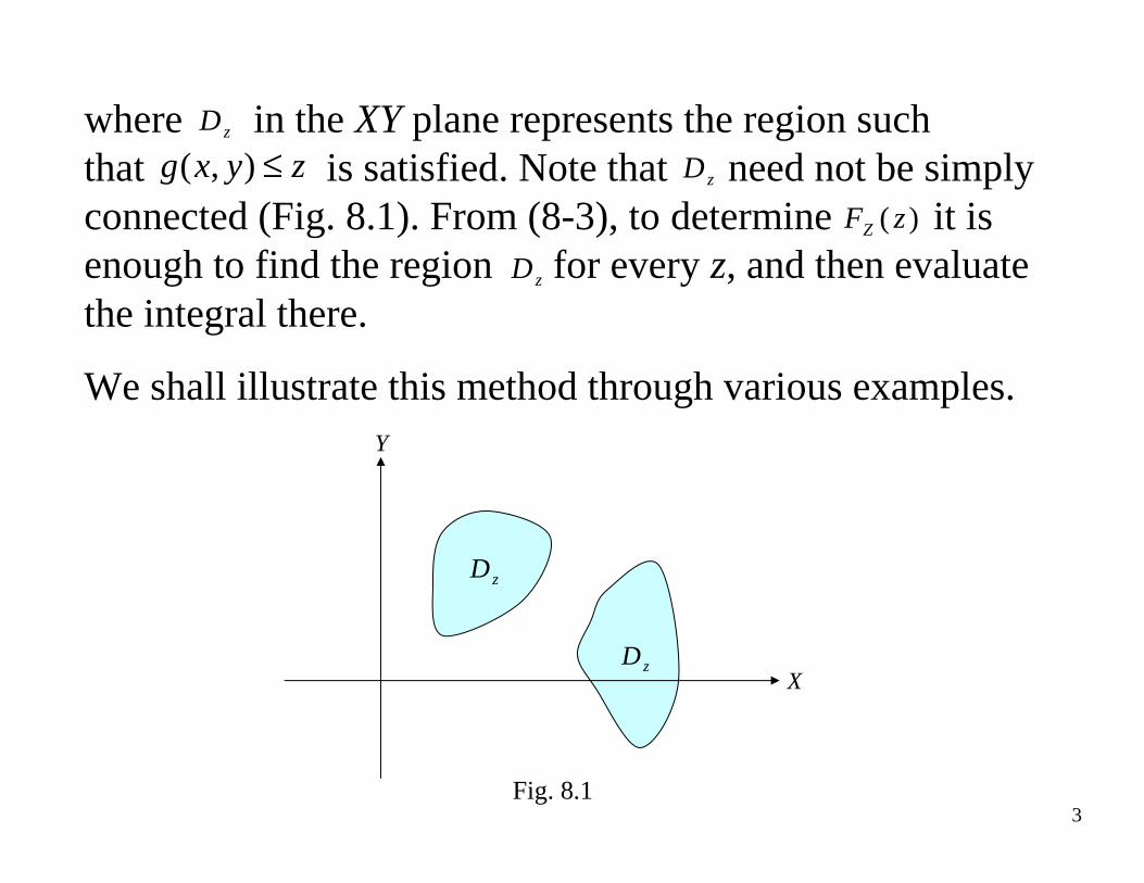
where in the XY plane represents the region such that is satisfied. Note that need not be simply connected (Fig. 8.1). From (8-3), to determine it is enough to find the region for every z, and then evaluate the integral there.

We shall illustrate this method through various examples.

zD

zyxg ≤),(

)( zFZ

zD

zD

X

Y

zD

zD

Fig. 8.1

4

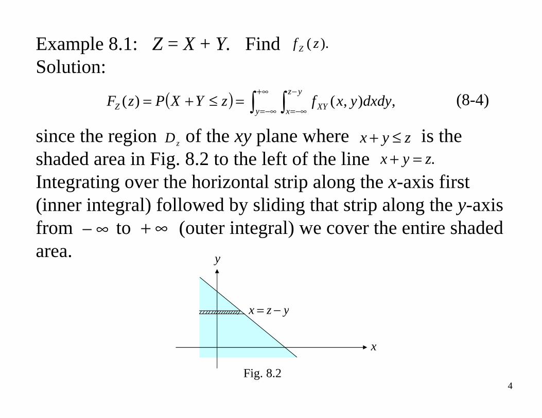
Example 8.1: Z = X + Y. Find Solution:

since the region of the xy plane where is the shaded area in Fig. 8.2 to the left of the line Integrating over the horizontal strip along the x-axis first (inner integral) followed by sliding that strip along the y-axis from to (outer integral) we cover the entire shaded area.

( ) ∫ ∫∞+

−∞=

−

−∞==≤+=

,),()(

y

yz

x XYZ dxdyyxfzYXPzF (8-4)

zD zyx ≤+.zyx =+

∞− ∞+

yzx −=

x

y

Fig. 8.2

).( zf Z

5

We can find by differentiating directly. In this context, it is useful to recall the differentiation rule in (7-15) - (7-16) due to Leibnitz. Suppose

Then

Using (8-6) in (8-4) we get

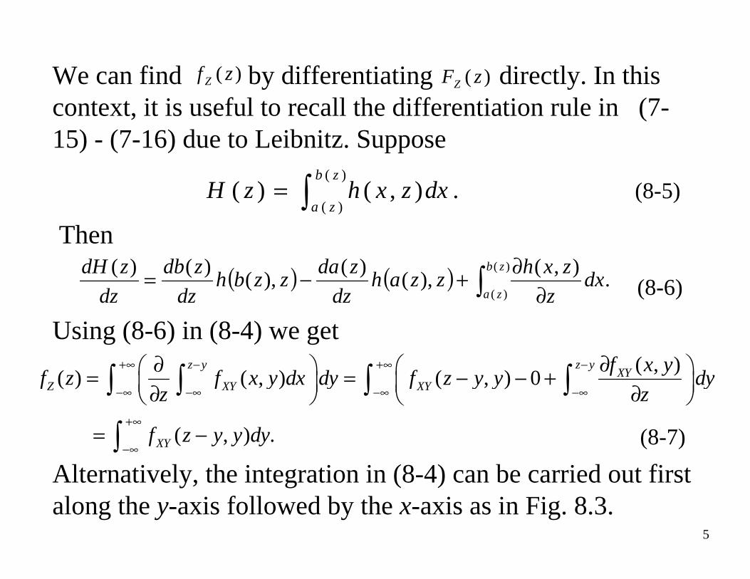
Alternatively, the integration in (8-4) can be carried out first along the y-axis followed by the x-axis as in Fig. 8.3.

)( zFZ)( zf Z

∫=)(

)( .),()(

zb

zadxzxhzH (8-5)

( ) ( ) ∫ ∂∂+−=

)(

)( .

),(),(

)(),(

)()( zb

zadx

z

zxhzzah

dz

zdazzbh

dz

zdb

dz

zdH(8-6)

( , )( ) ( , ) ( , ) 0

( , ) .

z y z yXY

Z XY XY

XY

f x yf z f x y dx dy f z y y dy

z z

f z y y dy

+∞ − +∞ −

−∞ −∞ −∞ −∞

+∞

−∞

∂∂ ⎛ ⎞⎛ ⎞= = − − +⎜ ⎟ ⎜ ⎟∂ ∂⎝ ⎠ ⎝ ⎠

= −

∫ ∫ ∫ ∫

∫ (8-7)

6

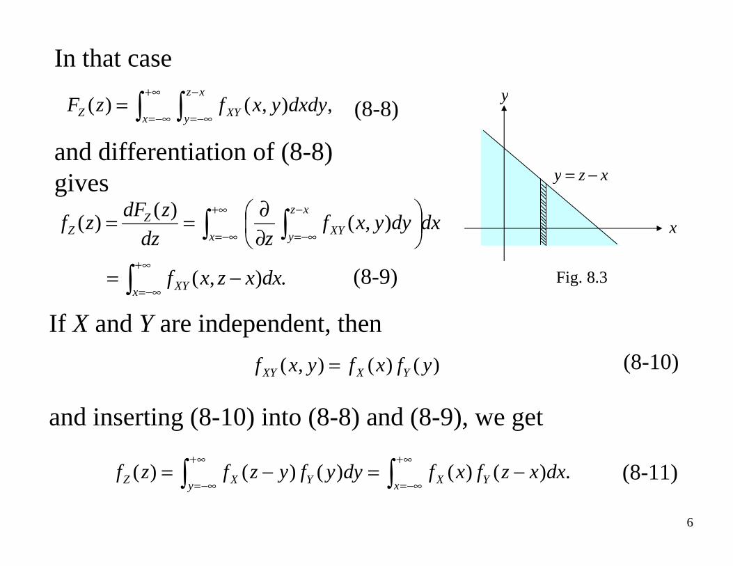
In that case

and differentiation of (8-8) gives

∫ ∫∞+

−∞=

−

−∞==

,),()(

x

xz

y XYZ dxdyyxfzF (8-8)

∫

∫ ∫∞+

−∞=

∞+

−∞=

−

−∞=

−=

⎟⎠⎞

⎜⎝⎛

∂∂==

.),(

),( )(

)(

x XY

x

xz

y XYZ

Z

dxxzxf

dxdyyxfzdz

zdFzf

(8-9)

If X and Y are independent, then

and inserting (8-10) into (8-8) and (8-9), we get

)()(),( yfxfyxf YXXY =

.)()()()()(

∫∫∞+

−∞=

∞+

−∞=−=−=

x YXy YXZ dxxzfxfdyyfyzfzf

(8-10)

(8-11)

xzy −=

x

y

Fig. 8.3

7

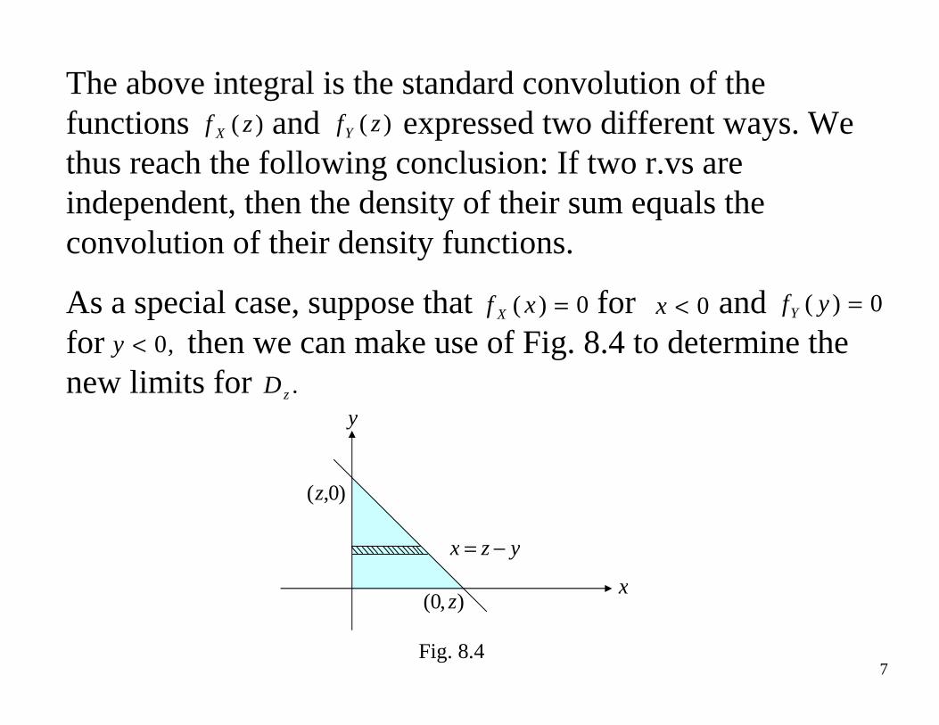
The above integral is the standard convolution of the functions and expressed two different ways. Wethus reach the following conclusion: If two r.vs are independent, then the density of their sum equals the convolution of their density functions.

As a special case, suppose that for and for then we can make use of Fig. 8.4 to determine the new limits for

)( zf X )( zfY

0)( =xf X 0<x 0)( =yfY

,0<y

.zD

Fig. 8.4

yzx −=

x

y

)0,(z

),0( z

8

In that case

or

On the other hand, by considering vertical strips first in Fig. 8.4, we get

or

if X and Y are independent random variables.

∫ ∫=

−

==

z

y

yz

x XYZ dxdyyxfzF

0

0 ),()(

⎪⎩

⎪⎨⎧

≤>−=⎟

⎠⎞

⎜⎝⎛

∂∂= ∫∫ ∫=

−

= .0,0

,0,),( ),()(

0

0

0 z

zdyyyzfdydxyxfz

zfz

XYz

y

yz

x XYZ (8-12)

⎪⎩

⎪⎨⎧

≤>−=−= ∫∫ =

= ,0,0

,0,)()(),()(

0

0 z

zdxxzfxfdxxzxfzf

z

y YXz

x XYZ

∫ ∫=

−

==

z

x

xz

y XYZ dydxyxfzF

0

0 ),()(

(8-13)

9

Example 8.2: Suppose X and Y are independent exponential r.vs with common parameter λ, and let Z = X + Y. Determine Solution: We have and we can make use of (13) to obtain the p.d.f of Z = X + Y.

As the next example shows, care should be taken in using the convolution formula for r.vs with finite range.

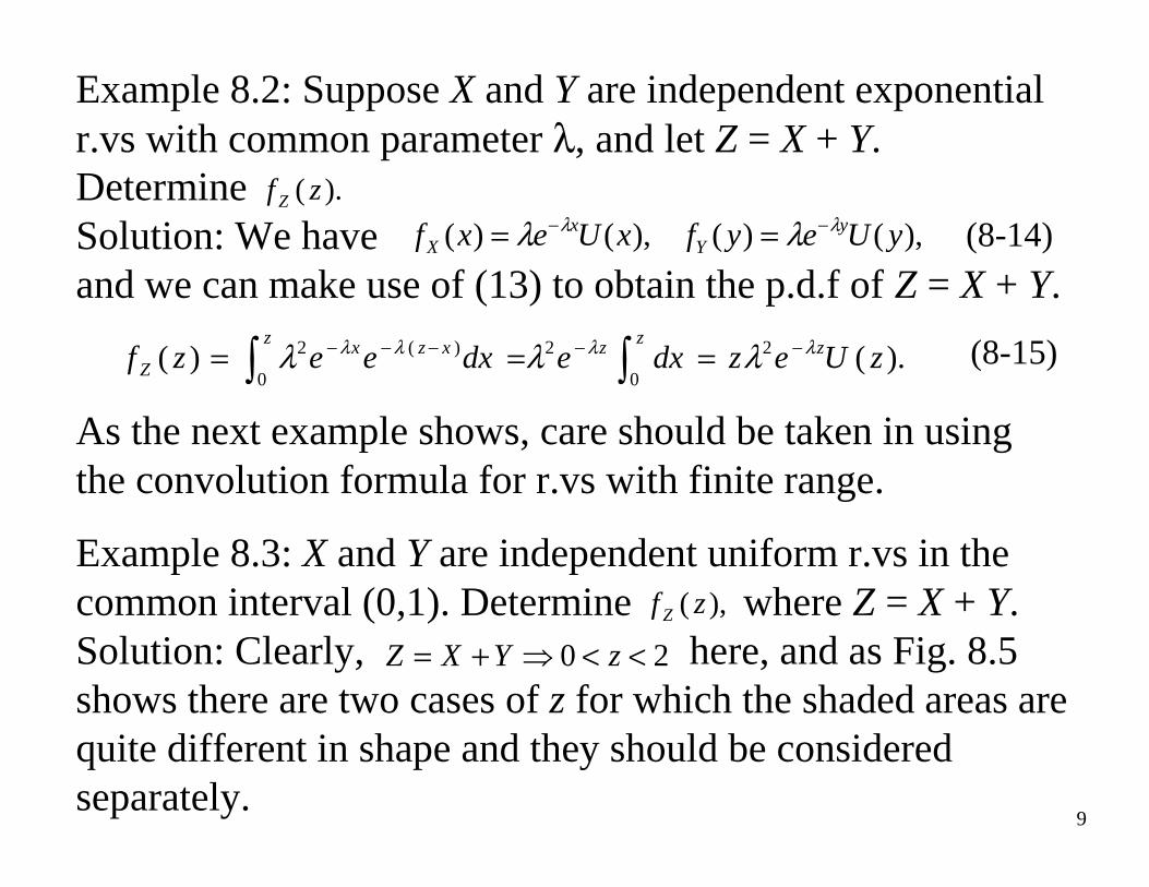
Example 8.3: X and Y are independent uniform r.vs in the common interval (0,1). Determine where Z = X + Y. Solution: Clearly, here, and as Fig. 8.5 shows there are two cases of z for which the shaded areas are quite different in shape and they should be considered separately.

),()( ),()( yUeyfxUexf yY

xX

λλ λλ −− == (8-14)

20 <<⇒+= zYXZ

),( zf Z

).( )( 2

0

2

0

)(2 zUezdxedxeezf zzzz xzxZ

λλλλ λλλ −−−−− === ∫∫ (8-15)

).( zf Z

10

x

y

yzx −=

10 )( << za

x

y

yzx −=

21 )( << zb

Fig. 8.5

For

For notice that it is easy to deal with the unshadedregion. In that case

,10 <≤ z

,21 <≤ z

.10 ,2

)( 1 )(2

0

0

0 <≤=−== ∫∫ ∫ ==

−

=z

zdyyzdxdyzF

z

y

z

y

yz

xZ(8-16)

( )

.21 ,2

)2(1)1(1

1 11)(

21

1z

1

1

1

<≤−−=+−−=

−=>−=

∫

∫ ∫

−=

−= −=

zz

dyyz

dxdyzZPzF

y

zy yzxZ

(8-17)

11

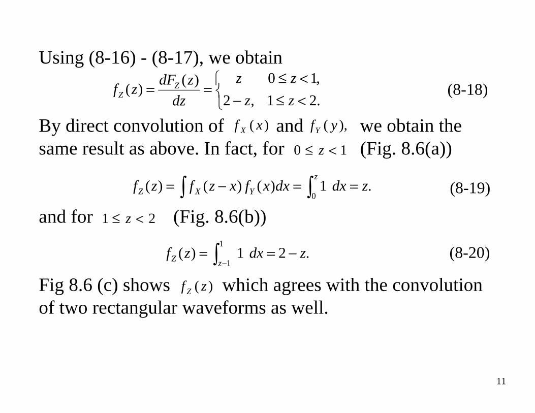
Using (8-16) - (8-17), we obtain

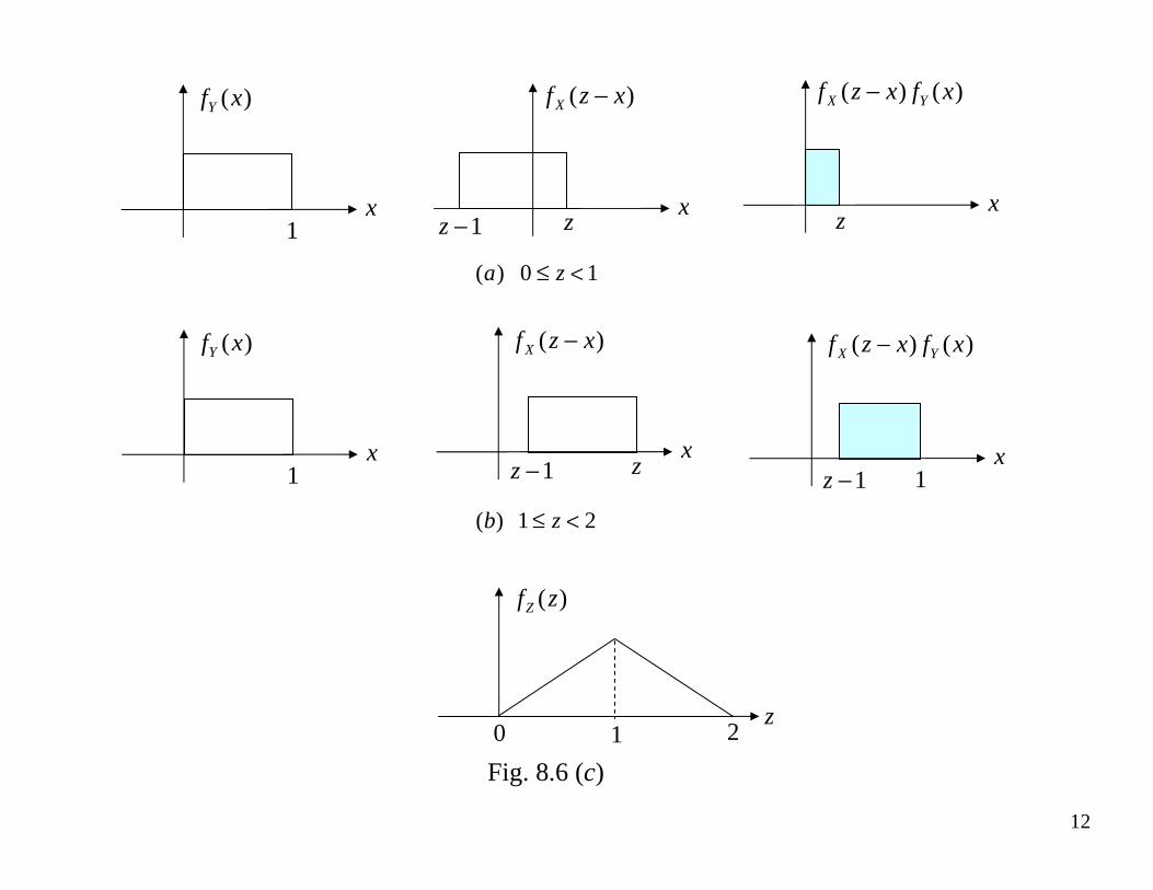
By direct convolution of and we obtain the same result as above. In fact, for (Fig. 8.6(a))

and for (Fig. 8.6(b))

Fig 8.6 (c) shows which agrees with the convolution of two rectangular waveforms as well.

⎩⎨⎧

<≤−<≤

==.21,2

,10)()(

zz

zz

dz

zdFzf Z

Z (8-18)

)( xf X ),( yfY

10 <≤ z

21 <≤ z

. 1 )()()(

0 zdxdxxfxzfzf

z

YXZ ==−= ∫ ∫

.2 1 )(1

1 zdxzf

zZ −== ∫ −

(8-19)

(8-20)

)( zf Z

12

)(xfY

x1

)( xzf X −

xz

)()( xfxzf YX −

xz1−z

10 )( <≤ za

)(xfY

x1

)( xzf X −

x

)()( xfxzf YX −

x11−z z

1−z

21 )( <≤ zb

Fig. 8.6 (c)

)(zfZ

z20 1

13

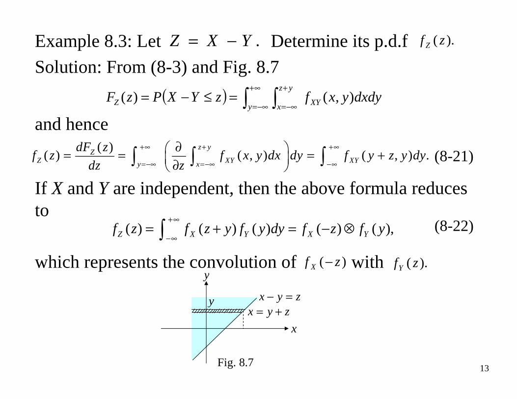
Example 8.3: Let Determine its p.d.f

Solution: From (8-3) and Fig. 8.7

and hence

If X and Y are independent, then the above formula reduces to

which represents the convolution of with

.YXZ −=

( ) ∫ ∫∞+

−∞=

+

−∞==≤−=

),( )(

y

yz

x XYZ dxdyyxfzYXPzF

( )( ) ( , ) ( , ) .

z yZ

Z XY XYy x

dF zf z f x y dx dy f y z y dy

dz z

+∞ + +∞

=−∞ =−∞ −∞

∂⎛ ⎞= = = +⎜ ⎟∂⎝ ⎠∫ ∫ ∫ (8-21)

( ) ( ) ( ) ( ) ( ),Z X Y X Yf z f z y f y dy f z f y

+∞

−∞= + = − ⊗∫ (8-22)

)( zf X − ).( zfY

Fig. 8.7

y

x

zyx =−zyx +=

y

).( zf Z

14

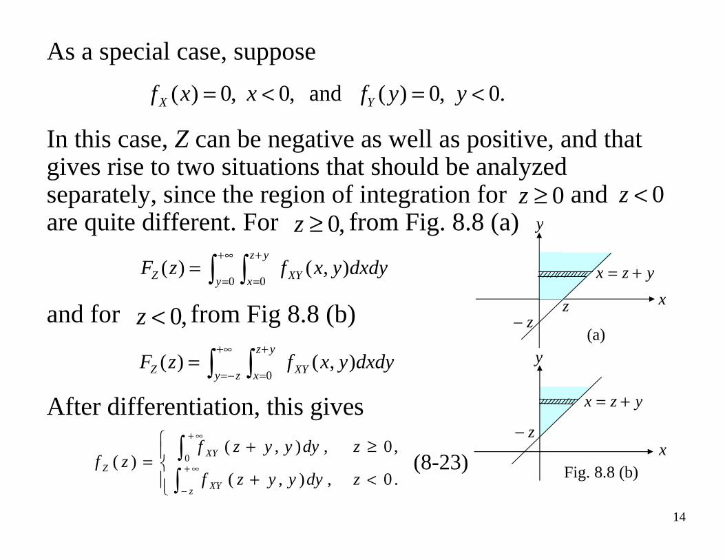
As a special case, suppose

In this case, Z can be negative as well as positive, and that gives rise to two situations that should be analyzed separately, since the region of integration for and are quite different. For from Fig. 8.8 (a)

and for from Fig 8.8 (b)

After differentiation, this gives

∫ ∫∞+

=

+

==

0

0 ),( )(

y

yz

x XYZ dxdyyxfzF

∫ ∫∞+

−=

+

==

0 ),( )(

zy

yz

x XYZ dxdyyxfzF

.0 ,0)( and ,0 ,0)( <=<= yyfxxf YX

0≥z 0<z,0≥z

,0<z

⎪⎩

⎪⎨⎧

<+

≥+=

∫∫

∞+

−

∞+

.0,),(

,0,),()(

0

zdyyyzf

zdyyyzfzf

z XY

XY

Z (8-23) Fig. 8.8 (b)

y

x

yzx +=

z−

y

x

yzx +=

zz−

(a)

15

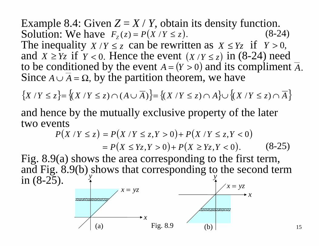
Example 8.4: Given Z = X / Y, obtain its density function.Solution: We have The inequality can be rewritten as if and if Hence the event in (8-24) need to be conditioned by the event and its compliment Since by the partition theorem, we have

and hence by the mutually exclusive property of the later two events

Fig. 8.9(a) shows the area corresponding to the first term, and Fig. 8.9(b) shows that corresponding to the second term in (8-25).

( ). /)( zYXPzFZ ≤= (8-24)zYX ≤/ YzX ≤ ,0>Y

YzX ≥ .0<Y ( )zYX ≤/( )0>= YA .

__

A__

,A A∪ = Ω

( ) ( ) ( )( ) ( ). 0,0,

0,/0,/ /

<≥+>≤=<≤+>≤=≤

YYzXPYYzXP

YzYXPYzYXPzYXP

(8-25)

Fig. 8.9

y

x

yzx =

(a)

y

xyzx =

(b)

AzYXAzYXAAzYXzYX ∩≤∪∩≤=∪∩≤=≤ )/()/()()/( /

16

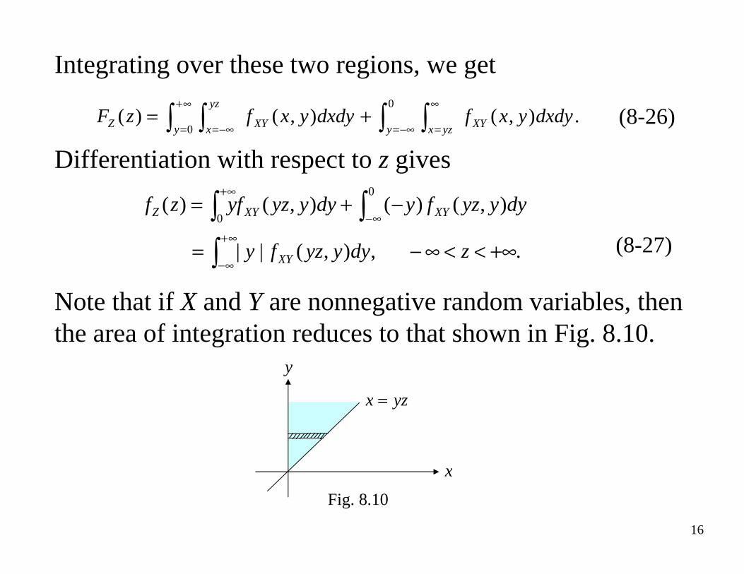
Integrating over these two regions, we get

Differentiation with respect to z gives

Note that if X and Y are nonnegative random variables, then the area of integration reduces to that shown in Fig. 8.10.

.),( ),( )(0

0

∫ ∫∫ ∫ −∞=

∞

=

∞+

= −∞=+=

y yzx XYy

yz

x XYZ dxdyyxfdxdyyxfzF (8-26)

. ,),(||

),()(),()(

0

0

+∞<<∞−=

−+=

∫∫∫

∞+

∞−

∞−

∞+

zdyyyzfy

dyyyzfydyyyzyfzf

XY

XYXYZ

(8-27)

y

x

yzx =

Fig. 8.10

17

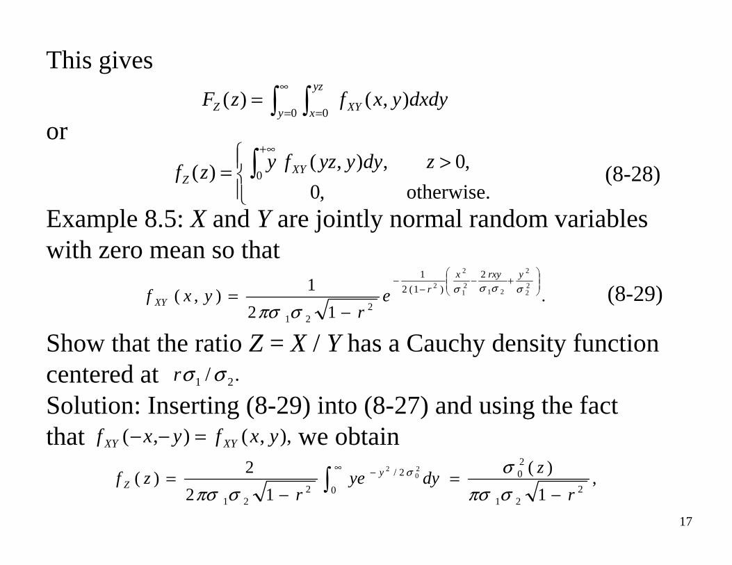
This gives

or

Example 8.5: X and Y are jointly normal random variables with zero mean so that

Show that the ratio Z = X / Y has a Cauchy density function centered at Solution: Inserting (8-29) into (8-27) and using the fact that we obtain

∫ ∫∞

= ==

0

0 ),( )(

y

yz

x XYZ dxdyyxfzF

⎪⎩

⎪⎨⎧ >= ∫

∞+

otherwise.,0

,0,),( )(

0 zdyyyzfyzf XY

Z (8-28)

.12

1),(

22

2

2121

2

2

2

)1(2

1

221

⎟⎟⎠

⎞⎜⎜⎝

⎛+−

−−

−= σσσσ

σπσ

yrxyx

rXY e

ryxf (8-29)

./ 21 σσr

,1

)(

12

2)(

221

20

0

2/

221

20

2

r

zdyye

rzf y

Z−

=−

= ∫∞ −

σπσσ

σπσσ

),,(),( yxfyxf XYXY =−−

18

where

Thus

which represents a Cauchy r.v centered at Integrating (8-30) from to z, we obtain the corresponding distribution function to be

Example 8.6: Obtain Solution: We have

.12

1)(

2221

21

2

220

σσσσ

σ+−

−=rzz

rz

,)1()/(

/1)( 22

12

2122

221

rrz

rzf Z −+−

−=σσσσ

πσσ (8-30)

./ 21 σσr

∞−

.1

arctan1

2

1)(

21

12

r

rzzFZ

−−+=

σσσ

π(8-31)

( ) .),()(22

22 ∫ ∫ ≤+=≤+=

zYX XYZ dxdyyxfzYXPzF

.22 YXZ +=

(8-32)

).( zf Z

19

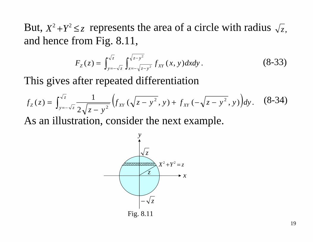
But, represents the area of a circle with radiusand hence from Fig. 8.11,

This gives after repeated differentiation

As an illustration, consider the next example.

zYX ≤+ 22,z

.),()(

2

2∫ ∫−=

−

−−==

z

zy

yz

yzx XYZ dxdyyxfzF (8-33)

( ) . ),(),(2

1)(

22

2∫ −=−−+−

−=

z

zy XYXYZ dyyyzfyyzfyz

zf (8-34)

Fig. 8.11

x

y

zzYX =+ 22

z

z−

20

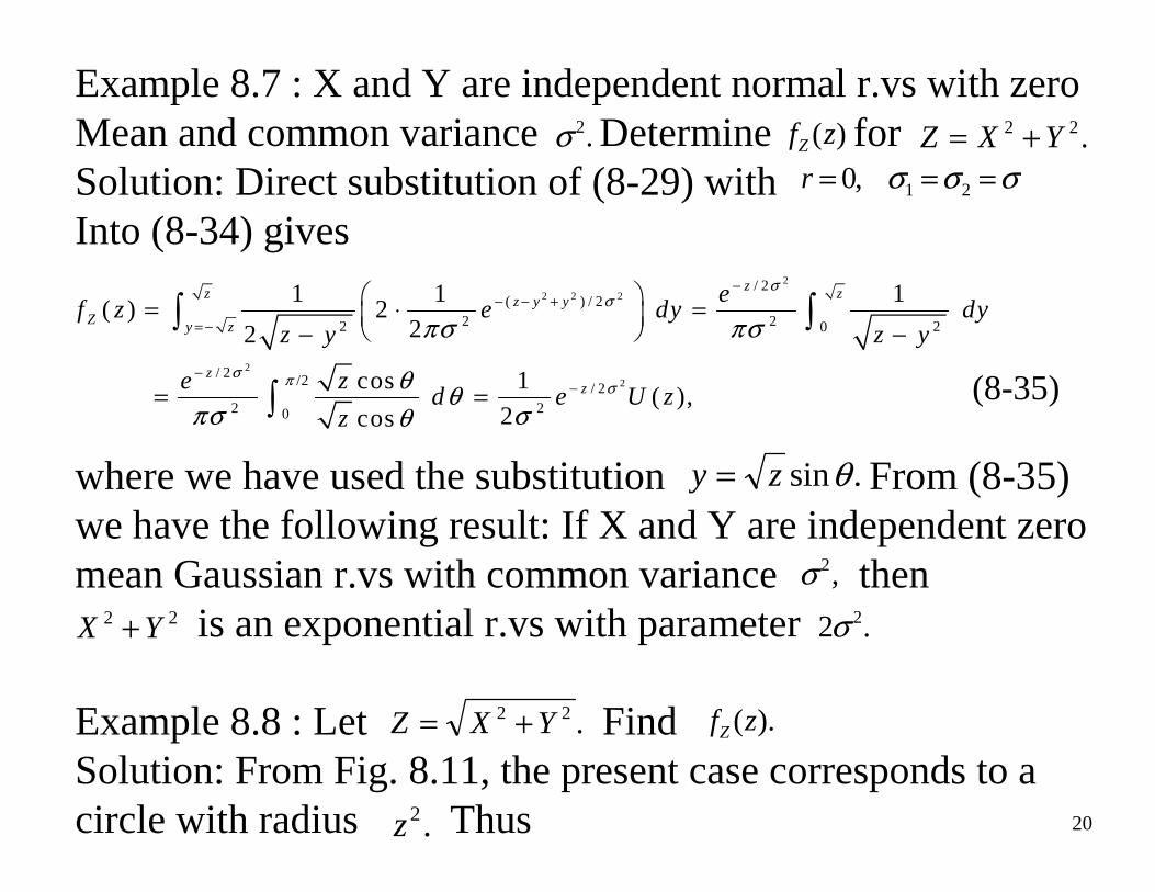
Example 8.7 : X and Y are independent normal r.vs with zeroMean and common variance Determine for Solution: Direct substitution of (8-29) with Into (8-34) gives

where we have used the substitution From (8-35)we have the following result: If X and Y are independent zeromean Gaussian r.vs with common variance then

is an exponential r.vs with parameter

Example 8.8 : Let Find Solution: From Fig. 8.11, the present case corresponds to a circle with radius Thus

)(zfZ .22 YXZ +=.2σσσσ === 21 ,0r

2

2 2 2

2

2

/ 2 ( ) / 22 22 2 0

/ 2 /2 / 22 2 0

1 1 1( ) 2

22

cos 1 ( ),

2cos

zz zz y yZ y z

zz

ef z e dy dy

z y z y

e zd e U z

z

σσ

σ π σ

πσ πσ

θ θπσ σθ

−− − +

= −

−−

⎛ ⎞= ⋅ =⎜ ⎟⎝ ⎠− −

= =

∫ ∫

∫ (8-35)

.sinθzy =

,2σ22 YX + .2 2σ

.22 YXZ += ).(zfZ

.2z

21

( ) . ),(),()(

2222

22∫ −−−+−

−=

z

z XYXYZ dyyyzfyyzfyz

zzf

.),()(

22

22∫ ∫−=

−

−−==

z

zy

yz

yzx XYZ dxdyyxfzF

),( cos

cos2

12

2

12)(

2222

222222

2/2

/2

0

2/2

0 22

2/2

0

2/)(222

zUez

dz

ze

z

dyyz

ez

dyeyz

zzf

zz

zzz yyzZ

σπσ

σσ

σθ

θθ

πσ

πσπσ

−−

−+−

==

−=

−=

∫

∫∫

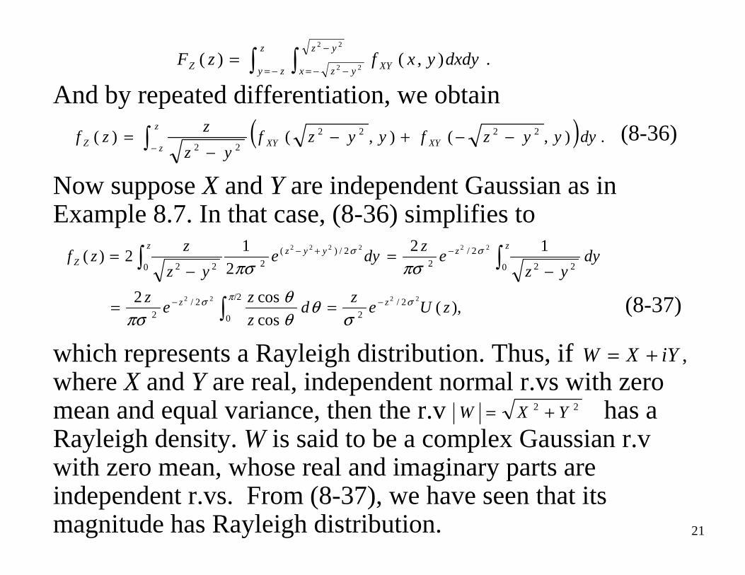
And by repeated differentiation, we obtain

Now suppose X and Y are independent Gaussian as in Example 8.7. In that case, (8-36) simplifies to

which represents a Rayleigh distribution. Thus, if where X and Y are real, independent normal r.vs with zero mean and equal variance, then the r.v has a Rayleigh density. W is said to be a complex Gaussian r.v with zero mean, whose real and imaginary parts are independent r.vs. From (8-37), we have seen that its magnitude has Rayleigh distribution.

(8-36)

(8-37)

,iYXW +=

22 YXW +=

22

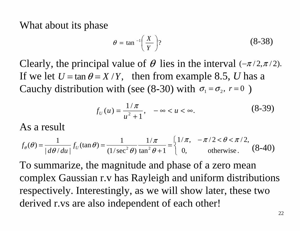
What about its phase

Clearly, the principal value of θ lies in the interval If we let then from example 8.5, U has a Cauchy distribution with (see (8-30) with )

As a result

To summarize, the magnitude and phase of a zero mean complex Gaussian r.v has Rayleigh and uniform distributions respectively. Interestingly, as we will show later, these two derived r.vs are also independent of each other!

?tan 1 ⎟⎠⎞

⎜⎝⎛= −

Y

Xθ (8-38)

. ,1

/1)(

2∞<<∞−

+= u

uufU

π (8-39)

).2/,2/( ππ−

tan / ,U X Yθ= =0 ,21 == rσσ

⎩⎨⎧ <<−

=+

==. otherwise,0

,2/2/,/1

1tan

/1

)sec/1(

1)(tan

|/|

1)(

22

πθππθπ

θθ

θθθ Ufdud

f (8-40)

23

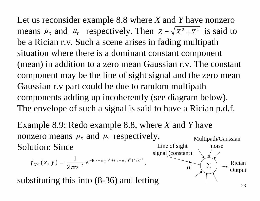
Let us reconsider example 8.8 where X and Y have nonzero means and respectively. Then is said to be a Rician r.v. Such a scene arises in fading multipathsituation where there is a dominant constant component (mean) in addition to a zero mean Gaussian r.v. The constant component may be the line of sight signal and the zero mean Gaussian r.v part could be due to random multipathcomponents adding up incoherently (see diagram below). The envelope of such a signal is said to have a Rician p.d.f.

Example 8.9: Redo example 8.8, where X and Y have nonzero means and respectively. Solution: Since

substituting this into (8-36) and letting

Xµ Yµ 22 YXZ +=

Xµ Yµ

,2

1),(

222 2/])()[(2

σµµ

πσYX yx

XY eyxf −+−−= RicianOutput

Line of sight signal (constant)

a

Multipath/Gaussian noise

∑

24

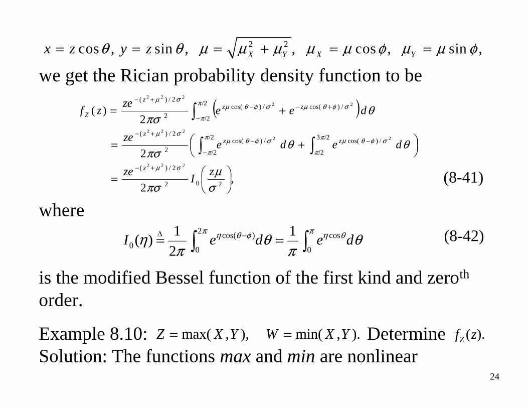
we get the Rician probability density function to be

where

is the modified Bessel function of the first kind and zeroth

order.

Example 8.10: Determine Solution: The functions max and min are nonlinear

2 2cos , sin , , cos , sin ,X Y X Yx z y zθ θ µ µ µ µ µ φ µ µ φ= = = + = =

( )

,2

2

2

)(

202

2/)(

/23

/2

/)cos(/2

/2

/)cos(2

2/)(

/2

/2

/)cos(/)cos(2

2/)(

222

22

222

22

222

⎟⎠⎞

⎜⎝⎛=

⎟⎠⎞⎜

⎝⎛ +=

+=

+−

−

−

−+−

−

+−−+−

∫∫

∫

σµ

πσ

θθπσ

θπσ

σµ

π

πσφθµπ

πσφθµ

σµ

π

πσφθµσφθµ

σµ

zI

ze

dedeze

deeze

zf

z

zzz

zzz

Z

∫∫ == − π θηπ φθη θπ

θπ

η

0

cos2

0

)cos(0

121

)( dedeI

(8-41)

).,min( ),,max( YXWYXZ ==

∆

).(zfZ

(8-42)

25

operators and represent special cases of the more general order statistics. In general, given any n-tuplewe can arrange them in an increasing order of magnitude such that

where and is the second smallest value among and finally If represent r.vs, the function that takes on the value in each possible sequence is known as the k-th order statistic. represent the set of order statistics among n random variables. In this context

represents the range, and when n = 2, we have the max and min statistics.

, , , , 21 nXXX

, )()2()1( nXXX ≤≤≤

( ) , , , , min 21)1( nXXXX = )2(X

, , , , 21 nXXX ( ). , , ,max 21)( nn XXXX =

nXXX , , , 21 )( kX

)( kx ( )nxxx , , , 21

)1()( XXR n −= (8-44)

(8-43)

(1) (2) ( )( , , , )nX X X

26

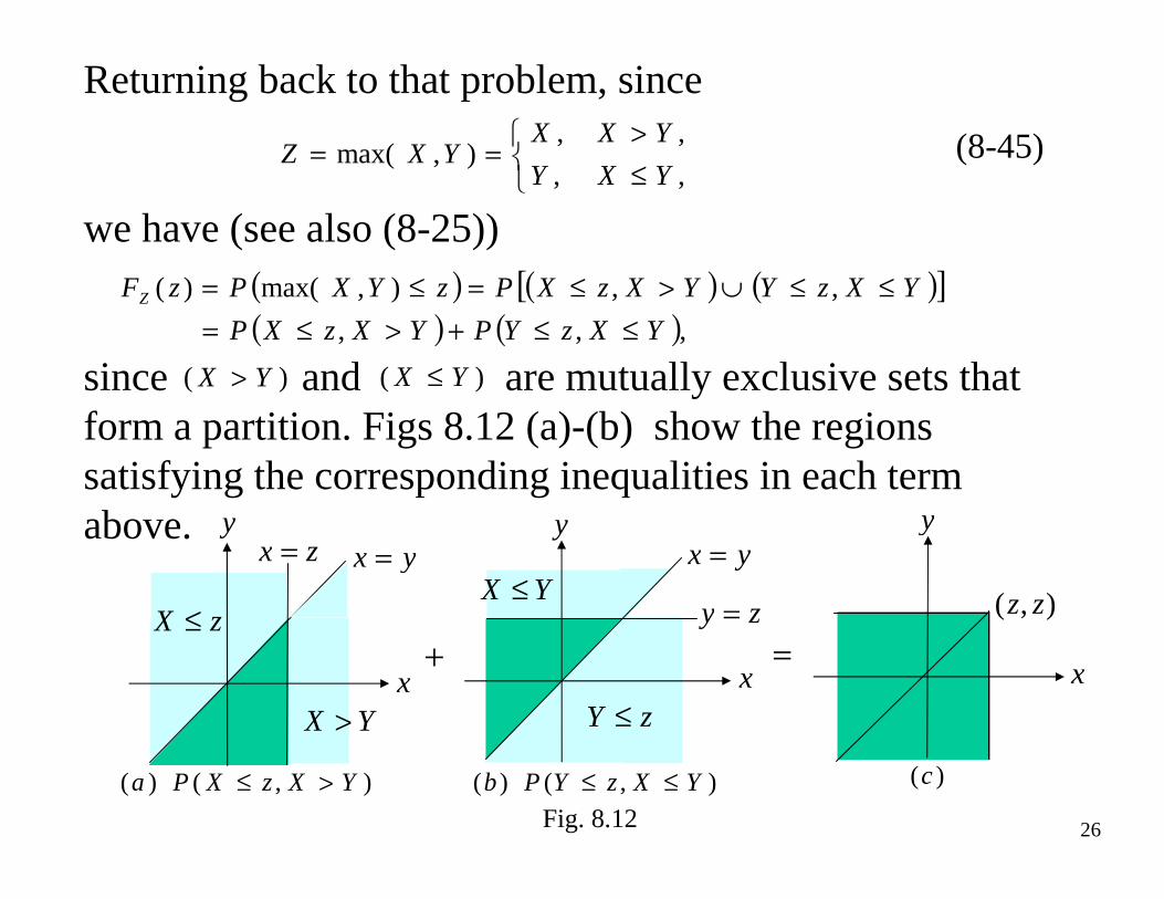
Returning back to that problem, since

we have (see also (8-25))

since and are mutually exclusive sets that form a partition. Figs 8.12 (a)-(b) show the regions satisfying the corresponding inequalities in each term above.

⎩⎨⎧

≤>

==,,

,,),max(

YXY

YXXYXZ (8-45)

( ) ( ) ( )[ ]( ) ( ),,,

,,),max()(

YXzYPYXzXP

YXzYYXzXPzYXPzFZ

≤≤+>≤=≤≤∪>≤=≤=

)( YX > )( YX ≤

x

yzx = yx =

zX ≤

YX >

),( )( YXzXPa >≤Fig. 8.12

x

y

zY ≤

YX ≤yx =

zy =

),( )( YXzYPb ≤≤

x

y

),( zz

)(c

+ =

27

(8-46)

Fig. 8.12 (c) represents the total region, and from there

If X and Y are independent, then

and hence

Similarly

Thus

( ) ).,(,)( zzFzYzXPzF XYZ =≤≤=

)()()( yFxFzF YXZ =

).()()()()( zFzfzfzFzf YXYXZ += (8-47)

⎩⎨⎧

≤>

==.,

,,),min(

YXX

YXYYXW (8-48)

( ) ( ) ( )[ ]. ,,),min()( YXwXYXwYPwYXPwFW ≤≤∪>≤=≤=

28

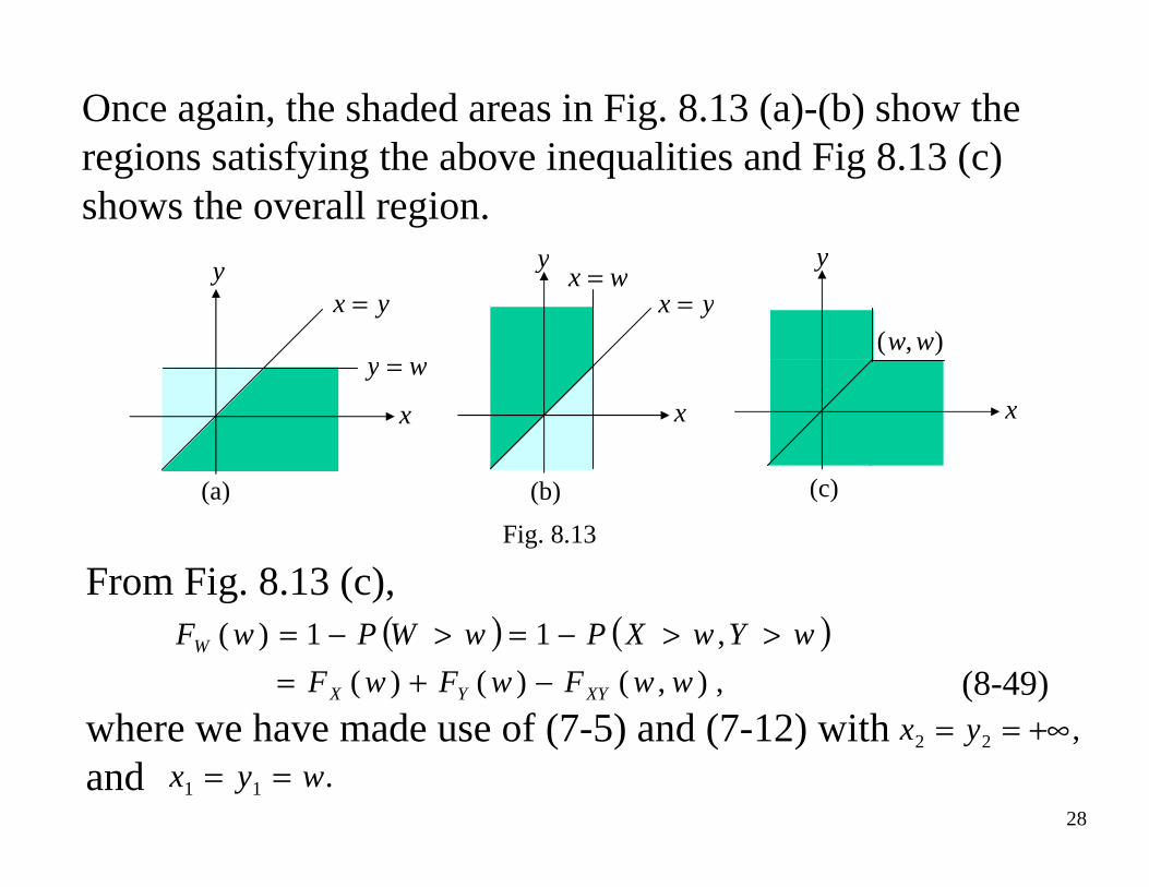
Once again, the shaded areas in Fig. 8.13 (a)-(b) show the regions satisfying the above inequalities and Fig 8.13 (c) shows the overall region.

From Fig. 8.13 (c),

where we have made use of (7-5) and (7-12) with and

( ) ( ), ),()()(

,11)(

wwFwFwF

wYwXPwWPwF

XYYX

W

−+=>>−=>−=

(8-49),22 +∞== yx

.11 wyx ==

x

yyx =

wy =

(a)

Fig. 8.13

x

y

yx =wx =

(b)

x

y

),( ww

(c)

29

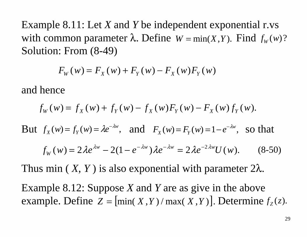
Example 8.11: Let X and Y be independent exponential r.vswith common parameter λ. Define Find Solution: From (8-49)

and hence

But and so that

Thus min ( X, Y ) is also exponential with parameter 2λ.

Example 8.12: Suppose X and Y are as give in the above example. Define Determine

).,min( YXW = ?)(wfW

)()()()( )( wFwFwFwFwF YXYXW −+=

).()()()()()( )( wfwFwFwfwfwfwf YXYXYXW −−+=

,)( )( wYX ewfwf λλ −== ,1)( )( w

YX ewFwF λ−−==

).(2)1(22 )( 2 wUeeeewf wwwwW

λλλλ λλλ −−− =−−= (8-50)

[ ]. ),max(/),min( YXYXZ = ).(zfZ

30

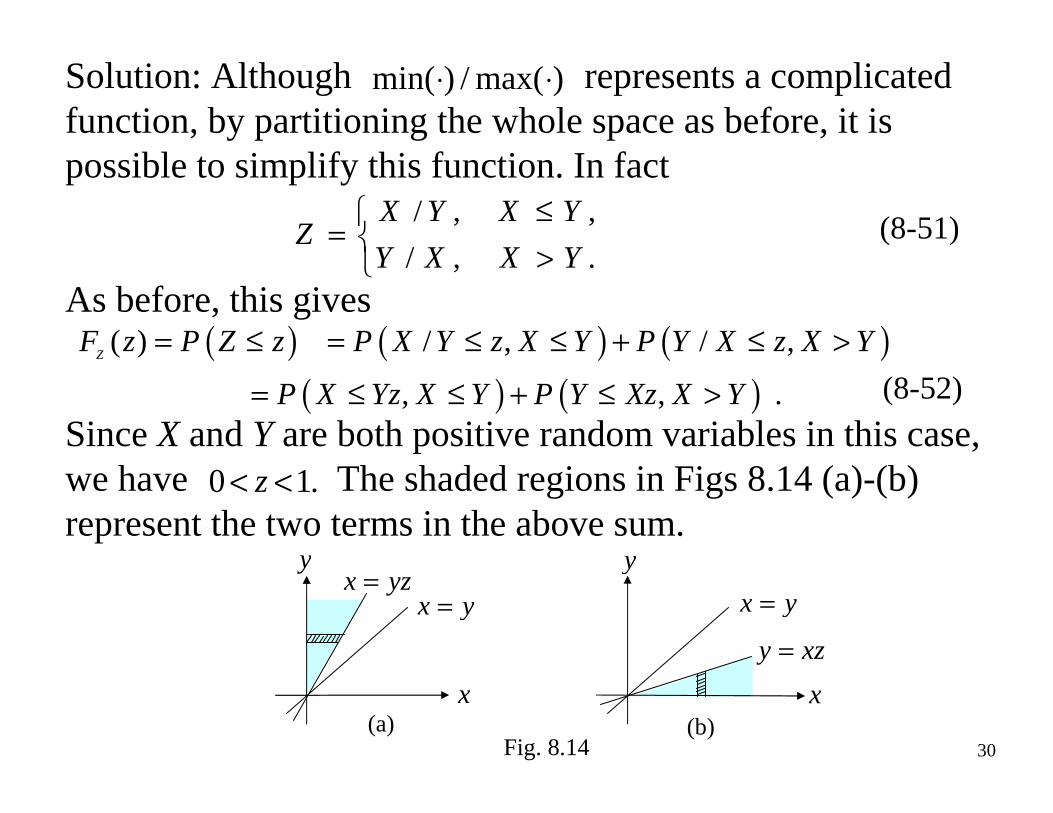
Solution: Although represents a complicated function, by partitioning the whole space as before, it is possible to simplify this function. In fact

As before, this gives

Since X and Y are both positive random variables in this case, we have The shaded regions in Figs 8.14 (a)-(b) represent the two terms in the above sum.

Fig. 8.14

)max(/)min( ⋅⋅

⎩⎨⎧

>≤

=.,/

,,/

YXXY

YXYXZ (8-51)

( ) ( ) ( )( ) ( )

( ) / , / ,

, , .

ZF z P Z z P X Y z X Y P Y X z X Y

P X Yz X Y P Y Xz X Y

= ≤ = ≤ ≤ + ≤ >

= ≤ ≤ + ≤ >

.10 << z

x

y

yx =yzx =

(a)x

y

yx =

xzy =

(b)

(8-52)

31

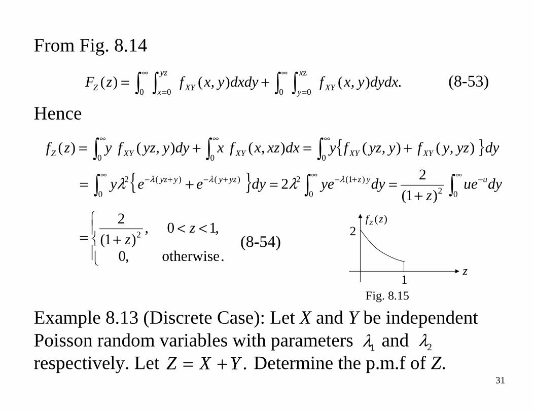
From Fig. 8.14

Hence

Example 8.13 (Discrete Case): Let X and Y be independent Poisson random variables with parameters and respectively. Let Determine the p.m.f of Z.

.),( ),( )(

0

z

0

0

0 ∫ ∫∫ ∫∞

=

∞

=+=

x

y XY

yz

x XYZ dydxyxfdxdyyxfzF

⎪⎩

⎪⎨⎧ <<

+=

+==+=

+=+=

∫∫∫

∫∫∫∞ −∞ +−∞ +−+−

∞∞∞

. otherwise,0

,10,)1(

2

)1(

22

),(),(),( ),( )(

2

0 2

0

)1(2

0

)()(2

0

0

0

zz

dyuez

dyyedyeey

dyyzyfyyzfydxxzxfxdyyyzfyzf

uyzyzyyyz

XYXYXYXYZ

λλλ λλ

(8-54)

1λ 2λ.YXZ +=

(8-53)

)(zfZ

z

Fig. 8.151

2

32

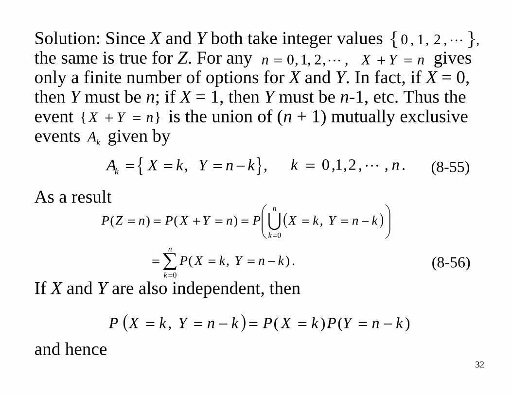
Solution: Since X and Y both take integer values the same is true for Z. For any gives only a finite number of options for X and Y. In fact, if X = 0, then Y must be n; if X = 1, then Y must be n-1, etc. Thus the event is the union of (n + 1) mutually exclusive events given by

As a result

If X and Y are also independent, then

and hence

, ,2 ,1 ,0 nYXn =+= , ,2 ,1 ,0

( )

. ) ,(

,)()(

0

0

∑=

=

−===

⎟⎟⎠

⎞⎜⎜⎝

⎛ −====+==

n

k

n

k

knYkXP

knYkXPnYXPnZP ∪

(8-55) , ,kA X k Y n k= = = −

( ) )()( , knYPkXPknYkXP −===−==

(8-56)

nYX =+

kA

.,,2,1,0 nk =

33

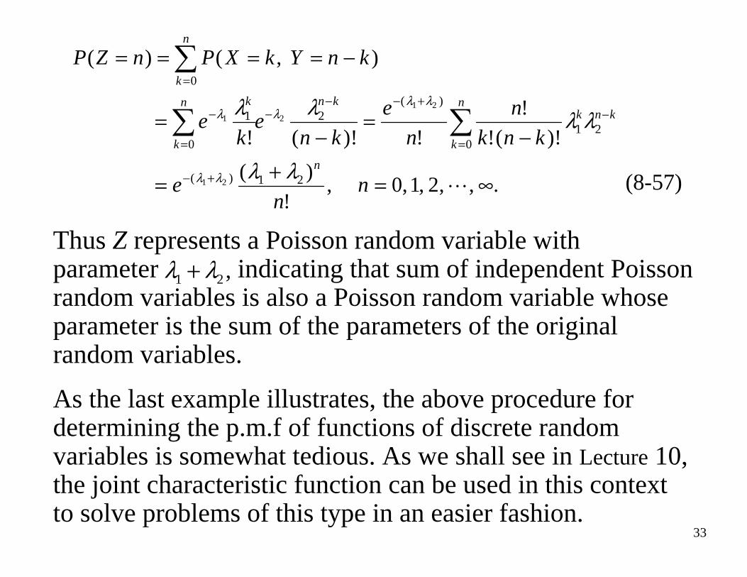
Thus Z represents a Poisson random variable with parameter indicating that sum of independent Poisson random variables is also a Poisson random variable whose parameter is the sum of the parameters of the original random variables.

As the last example illustrates, the above procedure for determining the p.m.f of functions of discrete random variables is somewhat tedious. As we shall see in Lecture 10, the joint characteristic function can be used in this context to solve problems of this type in an easier fashion.

,21 λλ +

. , ,2 ,1 ,0 ,!

)(

)!(!

!

!)!(!

) ,()(

21)(

021

)(2

0

1

0

21

21

21

∞=+=

−=

−=

−====

+−

=

−+−−

−

=

−

=

∑∑

∑

nn

e

knk

n

n

e

kne

ke

knYkXPnZP

n

n

k

knkknn

k

k

n

k

λλ

λλλλ

λλ

λλλλ

(8-57)