Geometry of the Lq-centroid bodies of an isotropic log-concave
YS – 2019-20 – C2
1
Lecture 2
Particle in an isotropic potential
- The angular momentum in Quantum Mechanics -
YS – 2019-20 – C2
2
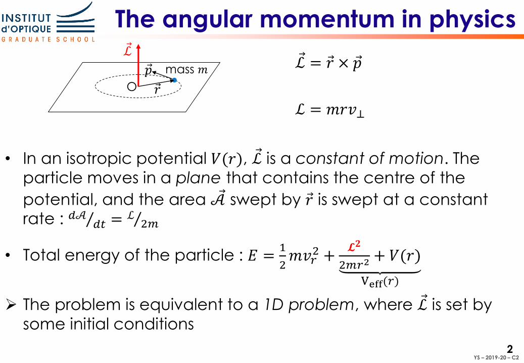
The angular momentum in physics
Ԧℒ = Ԧ𝑟 × Ԧ𝑝
ℒ = 𝑚𝑟𝑣⊥
• In an isotropic potential 𝑉(𝑟), Ԧℒ is a constant of motion. The
particle moves in a plane that contains the centre of the
potential, and the area Ԧ𝒜 swept by Ԧ𝑟 is swept at a constant rate : Τ𝑑𝒜
𝑑𝑡 = Τℒ 2𝑚
• Total energy of the particle : 𝐸 =1
2𝑚𝑣𝑟
2 +𝓛𝟐
2𝑚𝑟2+ 𝑉(𝑟)
Veff(𝑟)
The problem is equivalent to a 1D problem, where Ԧℒ is set by
some initial conditions
Ԧℒ
O
mass 𝑚
Ԧ𝑟
Ԧ𝑝
YS – 2019-20 – C2
3
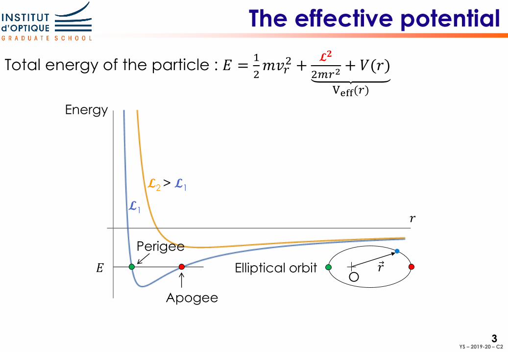
The effective potential
Total energy of the particle : 𝐸 =1
2𝑚𝑣𝑟
2 +𝓛𝟐
2𝑚𝑟2+ 𝑉(𝑟)
Veff(𝑟)
Energy
𝐸O
Elliptical orbit Ԧ𝑟
𝑟
Apogee
Perigee
𝓛1
𝓛2 > 𝓛1
YS – 2019-20 – C2
4
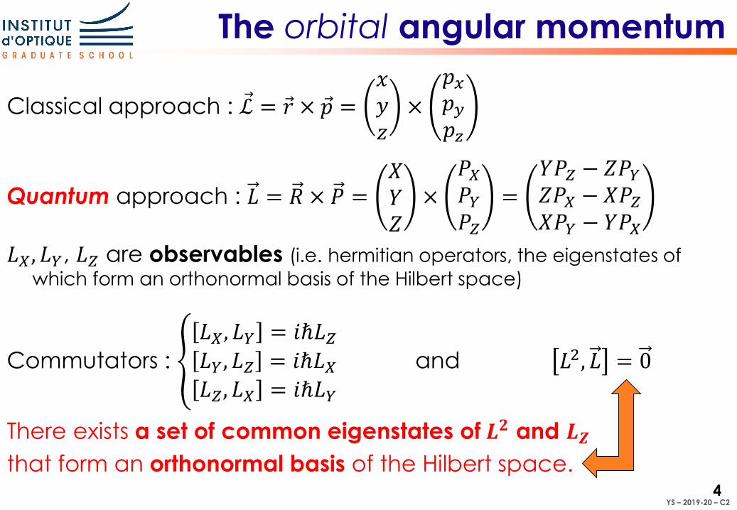
The orbital angular momentum
Classical approach : Ԧℒ = Ԧ𝑟 × Ԧ𝑝 =𝑥𝑦𝑧
×
𝑝𝑥𝑝𝑦𝑝𝑧
Quantum approach : 𝐿 = 𝑅 × 𝑃 =𝑋𝑌𝑍
×𝑃𝑋𝑃𝑌𝑃𝑍
=𝑌𝑃𝑍 − 𝑍𝑃𝑌𝑍𝑃𝑋 − 𝑋𝑃𝑍𝑋𝑃𝑌 − 𝑌𝑃𝑋
𝐿𝑋, 𝐿𝑌, 𝐿𝑍 are observables (i.e. hermitian operators, the eigenstates of
which form an orthonormal basis of the Hilbert space)
Commutators : ൞
𝐿𝑋, 𝐿𝑌 = 𝑖ℏ𝐿𝑍𝐿𝑌, 𝐿𝑍 = 𝑖ℏ𝐿𝑋𝐿𝑍, 𝐿𝑋 = 𝑖ℏ𝐿𝑌
and 𝐿2, 𝐿 = 0
There exists a set of common eigenstates of 𝑳𝟐 and 𝑳𝒁that form an orthonormal basis of the Hilbert space.
YS – 2019-20 – C2
5
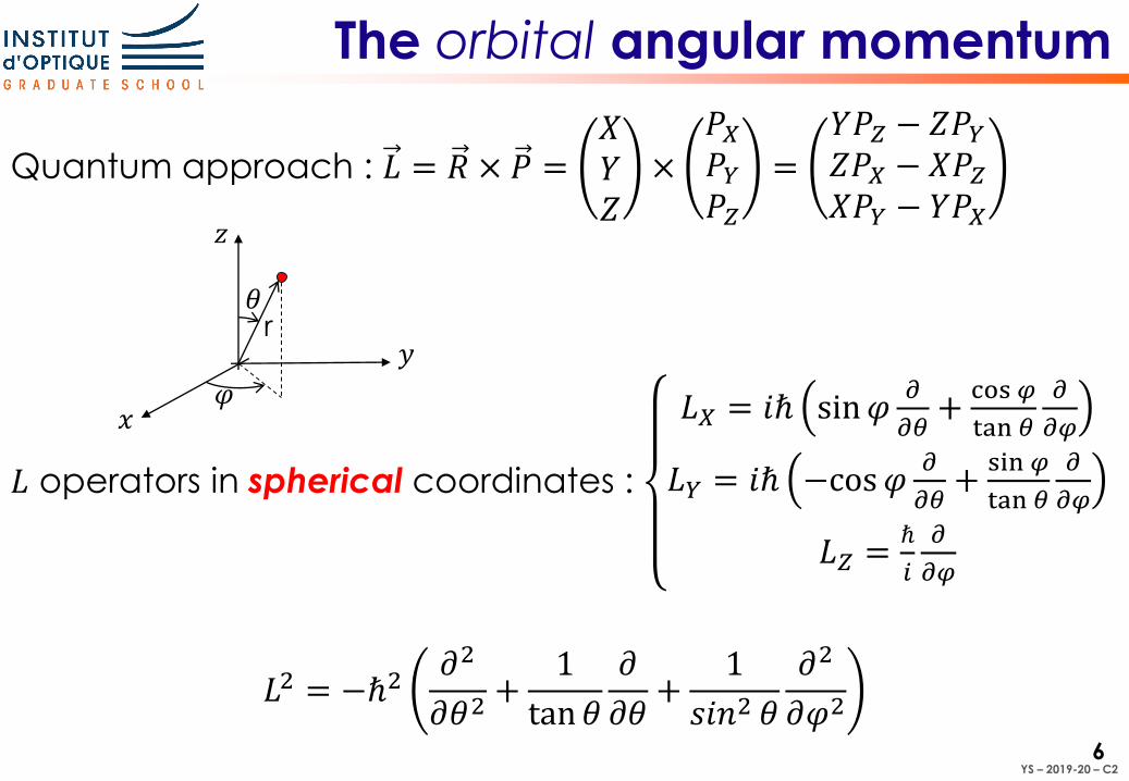
The orbital angular momentum
Quantum approach : 𝐿 = 𝑅 × 𝑃 =𝑋𝑌𝑍
×𝑃𝑋𝑃𝑌𝑃𝑍
=𝑌𝑃𝑍 − 𝑍𝑃𝑌𝑍𝑃𝑋 − 𝑋𝑃𝑍𝑋𝑃𝑌 − 𝑌𝑃𝑋
𝐿 operators in cartesian coordinates :
𝐿𝑋 =ℏ
𝑖𝑦
𝜕
𝜕𝑧− 𝑧
𝜕
𝜕𝑦
𝐿𝑌 =ℏ
𝑖𝑧
𝜕
𝜕𝑥− 𝑥
𝜕
𝜕𝑧
𝐿𝑍 =ℏ
𝑖𝑥
𝜕
𝜕𝑦− 𝑦
𝜕
𝜕𝑥
YS – 2019-20 – C2
6
The orbital angular momentum
Quantum approach : 𝐿 = 𝑅 × 𝑃 =𝑋𝑌𝑍
×𝑃𝑋𝑃𝑌𝑃𝑍
=𝑌𝑃𝑍 − 𝑍𝑃𝑌𝑍𝑃𝑋 − 𝑋𝑃𝑍𝑋𝑃𝑌 − 𝑌𝑃𝑋
𝐿 operators in spherical coordinates :
𝐿𝑋 = 𝑖ℏ sin𝜑𝜕
𝜕𝜃+
cos 𝜑
tan 𝜃
𝜕
𝜕𝜑
𝐿𝑌 = 𝑖ℏ −cos𝜑𝜕
𝜕𝜃+
sin 𝜑
tan 𝜃
𝜕
𝜕𝜑
𝐿𝑍 =ℏ
𝑖
𝜕
𝜕𝜑
𝐿2 = −ℏ2𝜕2
𝜕𝜃2+
1
tan 𝜃
𝜕
𝜕𝜃+
1
𝑠𝑖𝑛2 𝜃
𝜕2
𝜕𝜑2
r𝜃
𝜑𝑥
𝑦
𝑧
YS – 2019-20 – C2
7
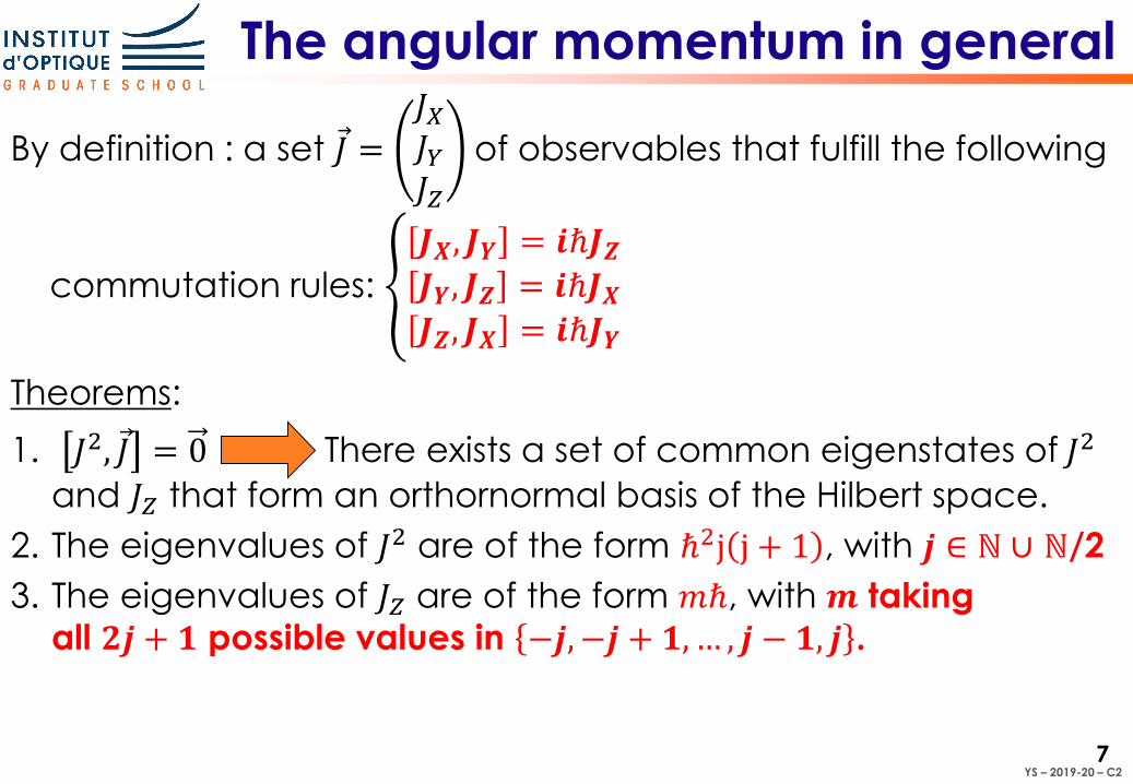
The angular momentum in general
By definition : a set Ԧ𝐽 =𝐽𝑋𝐽𝑌𝐽𝑍
of observables that fulfill the following
commutation rules: ൞
𝑱𝑿, 𝑱𝒀 = 𝒊ℏ𝑱𝒁𝑱𝒀, 𝑱𝒁 = 𝒊ℏ𝑱𝑿𝑱𝒁, 𝑱𝑿 = 𝒊ℏ𝑱𝒀
Theorems:
1. 𝐽2, Ԧ𝐽 = 0 There exists a set of common eigenstates of 𝐽2
and 𝐽𝑍 that form an orthornormal basis of the Hilbert space.
2. The eigenvalues of 𝐽2 are of the form ℏ2j j + 1 , with 𝒋 ∈ ℕ ∪ ℕ/2
3. The eigenvalues of 𝐽𝑍 are of the form 𝑚ℏ, with 𝒎 taking
all 𝟐𝒋 + 𝟏 possible values in −𝒋,−𝒋 + 𝟏,… , 𝒋 − 𝟏, 𝒋 .
YS – 2019-20 – C2
8
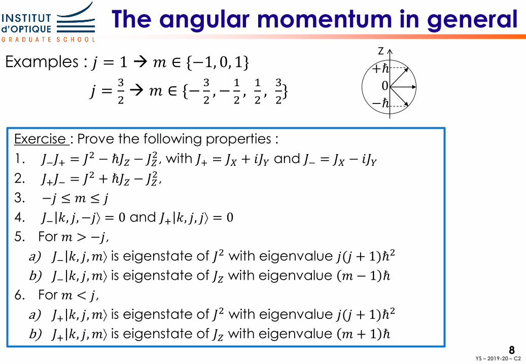
The angular momentum in general
Examples : 𝑗 = 1 𝑚 ∈ {−1, 0, 1}
𝑗 =3
2 𝑚 ∈ {−
3
2, −
1
2,1
2,3
2}
Exercise : Prove the following properties :
1. 𝐽−𝐽+ = 𝐽2 − ℏ𝐽𝑍 − 𝐽𝑍2, with 𝐽+ = 𝐽𝑋 + 𝑖𝐽𝑌 and 𝐽− = 𝐽𝑋 − 𝑖𝐽𝑌
2. 𝐽+𝐽− = 𝐽2 + ℏ𝐽𝑍 − 𝐽𝑍2,
3. −𝑗 ≤ 𝑚 ≤ 𝑗
4. 𝐽−ȁ𝑘, 𝑗, −𝑗 = 0 and 𝐽+ȁ𝑘, 𝑗, 𝑗 = 0
5. For 𝑚 > −𝑗,
a) 𝐽−ȁ𝑘, 𝑗,𝑚 is eigenstate of 𝐽2 with eigenvalue 𝑗(𝑗 + 1)ℏ2
b) 𝐽−ȁ𝑘, 𝑗,𝑚 is eigenstate of 𝐽𝑍 with eigenvalue 𝑚 − 1 ℏ
6. For 𝑚 < 𝑗,
a) 𝐽+ȁ𝑘, 𝑗,𝑚 is eigenstate of 𝐽2 with eigenvalue 𝑗(𝑗 + 1)ℏ2
b) 𝐽+ȁ𝑘, 𝑗,𝑚 is eigenstate of 𝐽𝑍 with eigenvalue 𝑚 + 1 ℏ
−ℏ
+ℏ
0
z
YS – 2019-20 – C2
9
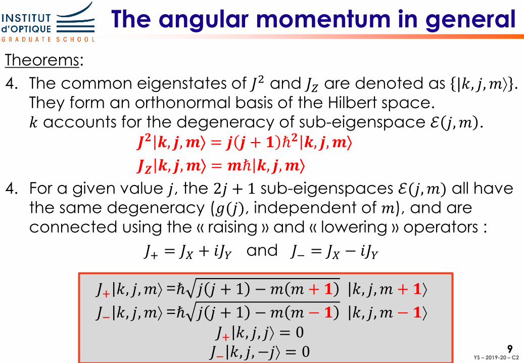
The angular momentum in general
Theorems:
4. The common eigenstates of 𝐽2 and 𝐽𝑍 are denoted as ȁ𝑘, 𝑗,𝑚 .
They form an orthonormal basis of the Hilbert space.
𝑘 accounts for the degeneracy of sub-eigenspace ℰ 𝑗,𝑚 .
𝑱𝟐ȁ𝒌, 𝒋,𝒎 = 𝒋 𝒋 + 𝟏 ℏ𝟐ȁ𝒌, 𝒋,𝒎
𝑱𝒁ȁ𝒌, 𝒋,𝒎 = 𝒎ℏȁ𝒌, 𝒋,𝒎
4. For a given value 𝑗, the 2𝑗 + 1 sub-eigenspaces ℰ(𝑗,𝑚) all have
the same degeneracy (𝑔(𝑗), independent of 𝑚), and are
connected using the « raising » and « lowering » operators :
𝐽+ = 𝐽𝑋 + 𝑖𝐽𝑌 and 𝐽− = 𝐽𝑋 − 𝑖𝐽𝑌
𝐽+ȁ𝑘, 𝑗,𝑚 =ℏ 𝑗 𝑗 + 1 −𝑚 𝑚 + 𝟏 ȁ𝑘, 𝑗,𝑚 + 𝟏
𝐽−ȁ𝑘, 𝑗,𝑚 =ℏ 𝑗 𝑗 + 1 −𝑚 𝑚 − 𝟏 ȁ𝑘, 𝑗,𝑚 − 𝟏𝐽+ȁ𝑘, 𝑗, 𝑗 = 0𝐽−ȁ𝑘, 𝑗, −𝑗 = 0
YS – 2019-20 – C2
10
Spectrum of the orbital angular momentum
Theorem : The eigenvalues of 𝐿2 are ℏ2𝑙 𝑙 + 1 , with 𝒍 ∈ ℕ
The common eigenstates of 𝐿2 and 𝐿𝑍 are denoted ȁ𝑙,𝑚.
Their associated wave functions in positions space are denoted𝜓 𝑟, 𝜃, 𝜑 = 𝑅 𝑟 𝑌𝑙
𝑚(𝜃, 𝜑)
Solve ൝𝐿2 𝑌𝑙
𝑚 𝜃, 𝜑 = 𝑙(𝑙 + 1)ℏ2 𝑌𝑙𝑚 𝜃, 𝜑
𝐿𝑍 𝑌𝑙𝑚 𝜃, 𝜑 = 𝑚ℏ 𝑌𝑙
𝑚 𝜃, 𝜑
Solutions : 𝑌𝑙𝑙 𝜃, 𝜑 = 𝑐𝑙 𝑠𝑖𝑛
𝑙𝜃 𝑒𝑖𝑙𝜑 with 𝑐𝑙 =(−1)𝑙
2𝑙 𝑙!
2𝑙+1 !
4𝜋
𝑌𝑙𝑚−1 𝜃, 𝜑 = 𝐿− 𝑌𝑙
𝑚 𝜃, 𝜑 /(ℏ 𝑙 𝑙 + 1 −𝑚(𝑚 − 1))
Radial part Angular part
« Spherical harmonic »න0
∞
𝑟2 𝑅 𝑟 2𝑑𝑟 = 1
න0
2𝜋
𝑑𝜑න0
𝜋
𝑑𝜃 sin 𝜃 𝑌𝑙𝑚 𝜃, 𝜑 2 = 1
YS – 2019-20 – C2
11
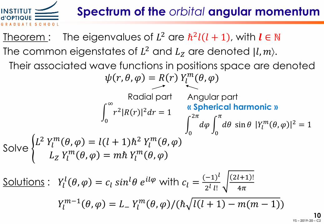
Spherical Harmonics
l = 0, m = 0
𝑌00 𝜃, 𝜑 =
1
4𝜋
Plot of 𝑌𝑙𝑚 𝜃, 𝜑
YS – 2019-20 – C2
12
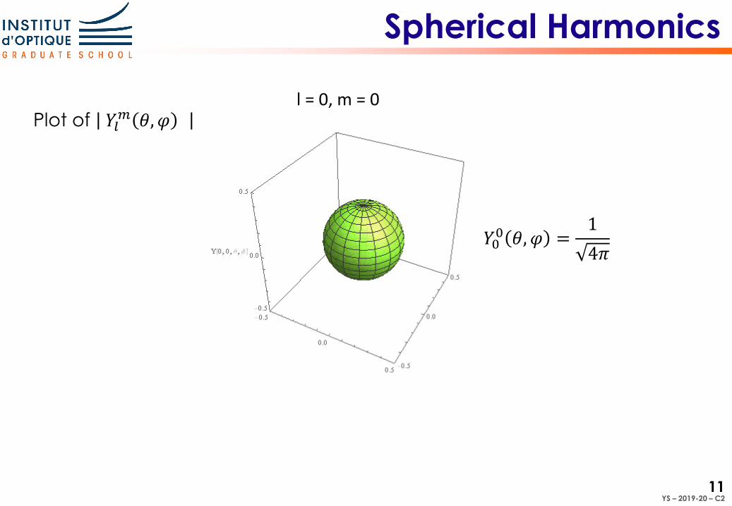
Spherical Harmonics
l = 1, m = 0 l = 1, m = 1
𝑌10 𝜃, 𝜑 =
3
4𝜋cos 𝜃 𝑌1
1 𝜃, 𝜑 = −3
8𝜋sin 𝜃 𝑒𝑖𝜑
Plot of 𝑌𝑙𝑚 𝜃, 𝜑
YS – 2019-20 – C2
13
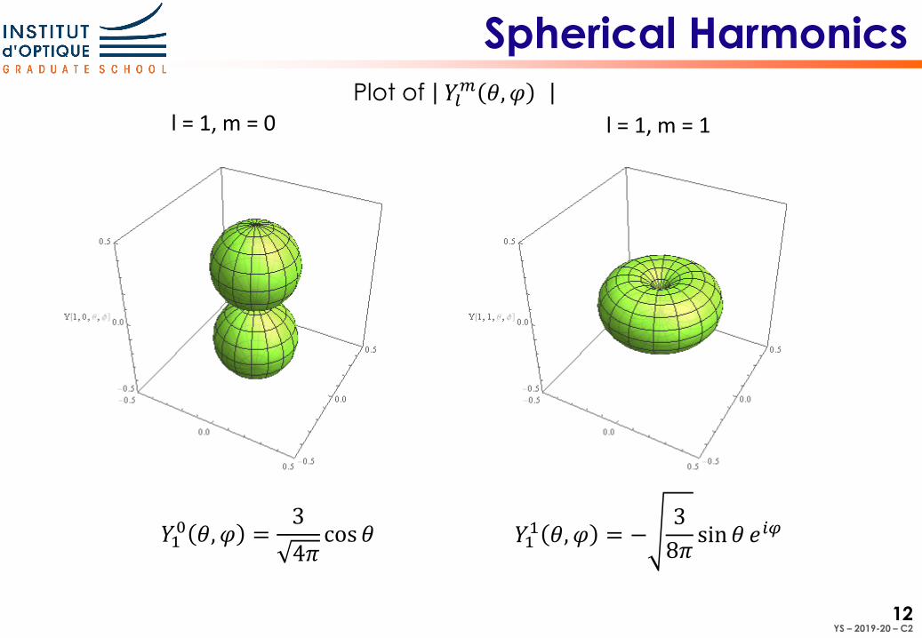
Spherical Harmonics
l = 2, m = 0 l = 2, m = 2l = 2, m = 1
𝑌20 𝜃, 𝜑 =
5
16𝜋(3𝑐𝑜𝑠2 𝜃 − 1) 𝑌2
1 𝜃, 𝜑 = −15
8𝜋sin 𝜃 cos 𝜃 𝑒𝑖𝜑 𝑌2
2 𝜃, 𝜑 =15
32𝜋𝑠𝑖𝑛2 𝜃 𝑒𝑖2𝜑
Plot of 𝑌𝑙𝑚 𝜃, 𝜑
YS – 2019-20 – C2
14
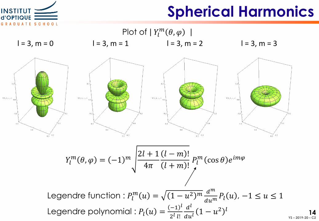
Spherical Harmonics
l = 3, m = 0 l = 3, m = 2l = 3, m = 1 l = 3, m = 3
Plot of 𝑌𝑙𝑚 𝜃, 𝜑
𝑌𝑙𝑚 𝜃, 𝜑 = −1 𝑚
2𝑙 + 1
4𝜋
𝑙 − 𝑚 !
𝑙 + 𝑚 !𝑃𝑙𝑚 cos 𝜃 𝑒𝑖𝑚𝜑
Legendre function : 𝑃𝑙𝑚 𝑢 = 1 − 𝑢2 𝑚 𝑑𝑚
𝑑𝑢𝑚𝑃𝑙 𝑢 , −1 ≤ 𝑢 ≤ 1
Legendre polynomial : 𝑃𝑙 𝑢 =−1 𝑙
2𝑙 𝑙!
𝑑𝑙
𝑑𝑢𝑙1 − 𝑢2 𝑙
YS – 2019-20 – C2
15
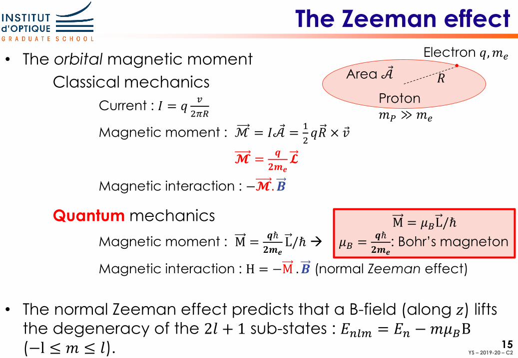
The Zeeman effect
• The orbital magnetic moment
Classical mechanics
Current : 𝐼 = 𝑞𝑣
2𝜋𝑅
Magnetic moment : ℳ = 𝐼 Ԧ𝒜 =1
2𝑞𝑅 × Ԧ𝑣
𝓜=𝒒
𝟐𝒎𝒆𝓛
Magnetic interaction : −𝓜.𝑩
Quantum mechanics
Magnetic moment : M =𝒒ℏ
𝟐𝒎𝒆L/ℏ
Magnetic interaction : H = −M .𝑩 (normal Zeeman effect)
• The normal Zeeman effect predicts that a B-field (along 𝑧) lifts
the degeneracy of the 2𝑙 + 1 sub-states : 𝐸𝑛𝑙𝑚 = 𝐸𝑛 −𝑚𝜇𝐵B(−l ≤ 𝑚 ≤ 𝑙).
Proton
𝑚𝑃 ≫ 𝑚𝑒
Electron 𝑞,𝑚𝑒
𝑅Area Ԧ𝒜
M = 𝜇𝐵L/ℏ
𝜇𝐵 =𝒒ℏ
𝟐𝒎𝒆: Bohr’s magneton
YS – 2019-20 – C2
16
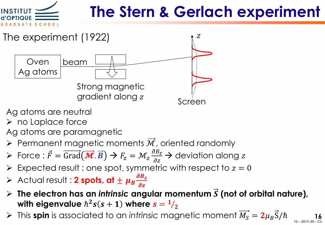
The Stern & Gerlach experiment
The experiment (1922)
Oven
Ag atoms
𝑧
Strong magnetic
gradient along 𝑧
beam
Ag atoms are neutral
no Laplace forceAg atoms are paramagnetic
Permanent magnetic moments ℳ, oriented randomly
Force : Ԧ𝐹 = Grad 𝓜.𝑩 𝐹𝑧 =ℳ𝑧𝜕𝐵𝑧
𝜕𝑧 deviation along 𝑧
Expected result : one spot, symmetric with respect to 𝑧 = 0
Actual result : 2 spots, at ± 𝝁𝑩𝝏𝑩𝒛
𝝏𝒛
The electron has an intrinsic angular momentum 𝑺 (not of orbital nature),
with eigenvalue ℏ𝟐𝒔 𝒔 + 𝟏 where 𝒔 = Τ𝟏 𝟐
This spin is associated to an intrinsic magnetic moment 𝑀𝑆 = 𝟐𝜇𝐵S/ℏ
Screen
YS – 2019-20 – C2
17
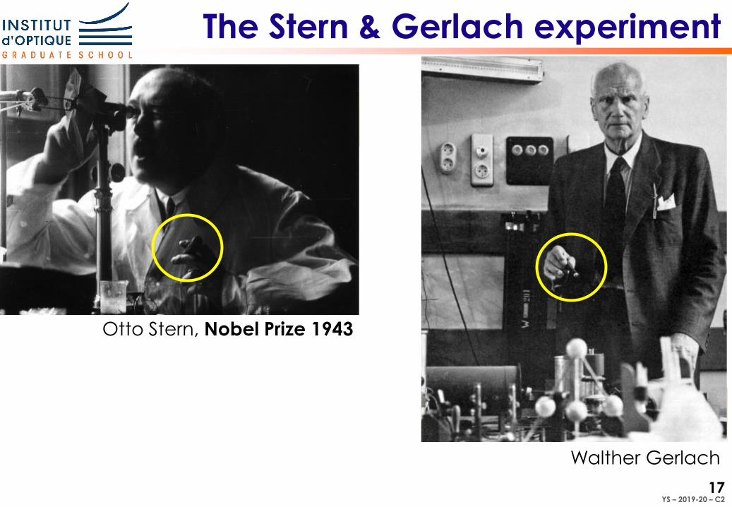
The Stern & Gerlach experiment
Otto Stern, Nobel Prize 1943
Walther Gerlach
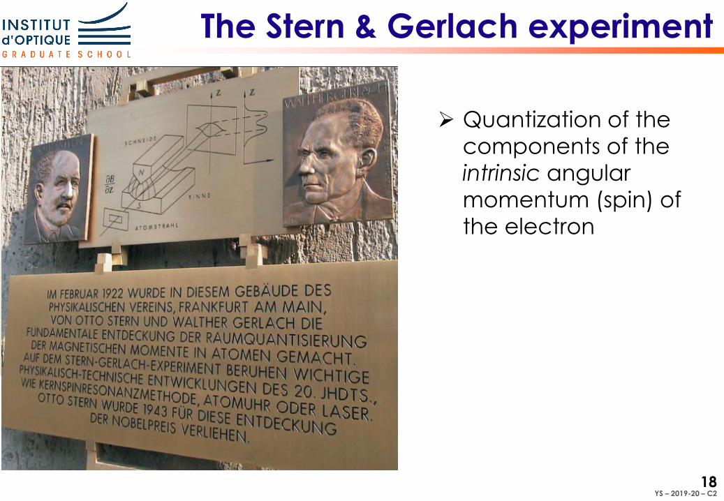
YS – 2019-20 – C2
18
The Stern & Gerlach experiment
Quantization of the
components of the
intrinsic angular
momentum (spin) of
the electron
YS – 2019-20 – C2
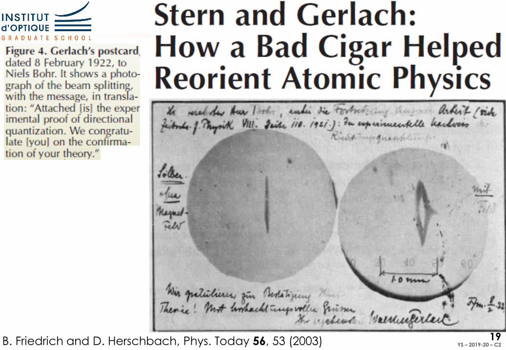
19B. Friedrich and D. Herschbach, Phys. Today 56, 53 (2003)
YS – 2019-20 – C2
20
To read more …
• On the angular momentum in quantum mechanics : CDL1, chapter VI
• On the spherical harmonics : CDL1, compl. AVI
• On Bohr’s model : CPP1, chapters I and VI
• On the spin of the electron and the Stern & Gerlach experiment :
TB, chapter VI; CDL1, chapters IV and IX; CPP1, chapter X
CDL1 : Cohen-Tannoudji, Diu, Laloë, Quantum Mechanics, volume 1TB : Tualle-Brouri, Introduction à la Mécanique Quantique, Cours 1A de l’IOGS
CPP1&2 : Cagnac, Pebay-Peyroula, Atomic physics, volumes 1 & 2
YS – 2019-20 – C2
21
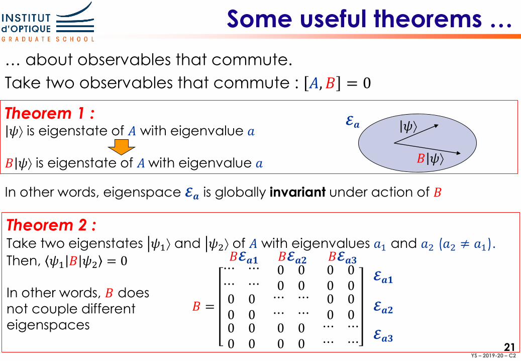
… about observables that commute.
Take two observables that commute : 𝐴, 𝐵 = 0
In other words, eigenspace 𝓔𝒂 is globally invariant under action of 𝐵
Theorem 1 : ȁ𝜓 is eigenstate of 𝐴 with eigenvalue 𝑎
𝐵ȁ𝜓 is eigenstate of 𝐴 with eigenvalue 𝑎
Some useful theorems …
ȁ𝜓
𝐵ȁ𝜓
𝓔𝒂
Theorem 2 : Take two eigenstates ห𝜓1 and ห𝜓2 of 𝐴 with eigenvalues 𝑎1 and 𝑎2 (𝑎2 ≠ 𝑎1).
Then, 𝜓1 𝐵 𝜓2 = 0
In other words, 𝐵 does
not couple different
eigenspaces
𝐵 =
⋯ ⋯⋯ ⋯
0 00 0
0 00 0
0 00 0
⋯ ⋯⋯ ⋯
0 00 0
0 00 0
0 00 0
⋯ ⋯⋯ ⋯
𝓔𝒂𝟏
𝓔𝒂𝟐
𝓔𝒂𝟑
𝐵𝓔𝒂𝟐𝐵𝓔𝒂𝟏 𝐵𝓔𝒂𝟑
YS – 2019-20 – C2
22
… about observables that commute.
Take two observables that commute : 𝐴, 𝐵 = 0
Some useful theorems …
Theorem 3 : There exists a set of common eigenstates of 𝐴 and 𝐵 that form an orthonormal
basis of the Hilbert space.


![surpass all possibilities - Waters Corporation · surpass all possibilities [ CORTECS 2.7 µm COLUMNS ] A SOLID-CORE PARTICLE COLUMN THAT LIVES UP TO ITS POTENTIAL. 2.7 m SLIDCORE](https://static.fdocument.org/doc/165x107/5e87c3eaed583a7aec5a497b/surpass-all-possibilities-waters-corporation-surpass-all-possibilities-cortecs.jpg)