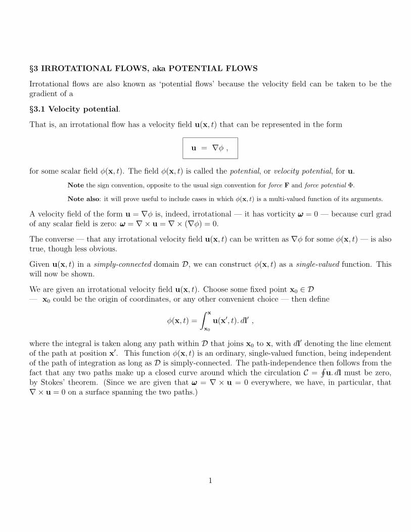
§3 IRROTATIONAL FLOWS, aka POTENTIAL FLOWS

Irrotational flows are also known as ‘potential flows’ because the velocity field can be taken to be thegradient of a

§3.1 Velocity potential.

That is, an irrotational flow has a velocity field u(x, t) that can be represented in the form

u = ∇φ ,

for some scalar field φ(x, t). The field φ(x, t) is called the potential, or velocity potential, for u.

Note the sign convention, opposite to the usual sign convention for force F and force potential Φ.

Note also: it will prove useful to include cases in which φ(x, t) is a multi-valued function of its arguments.

A velocity field of the form u = ∇φ is, indeed, irrotational — it has vorticity ωωω = 0 — because curl gradof any scalar field is zero: ωωω = ∇× u = ∇× (∇φ) = 0.

The converse — that any irrotational velocity field u(x, t) can be written as ∇φ for some φ(x, t) — is alsotrue, though less obvious.

Given u(x, t) in a simply-connected domain D, we can construct φ(x, t) as a single-valued function. Thiswill now be shown.

We are given an irrotational velocity field u(x, t). Choose some fixed point x0 ∈ D— x0 could be the origin of coordinates, or any other convenient choice — then define

φ(x, t) =

∫ x

x0

u(x′, t). dl′ ,

where the integral is taken along any path within D that joins x0 to x, with dl′ denoting the line elementof the path at position x′. This function φ(x, t) is an ordinary, single-valued function, being independentof the path of integration as long as D is simply-connected. The path-independence then follows from thefact that any two paths make up a closed curve around which the circulation C =

∮u. dl must be zero,

by Stokes’ theorem. (Since we are given that ωωω = ∇ × u = 0 everywhere, we have, in particular, that∇× u = 0 on a surface spanning the two paths.)

1

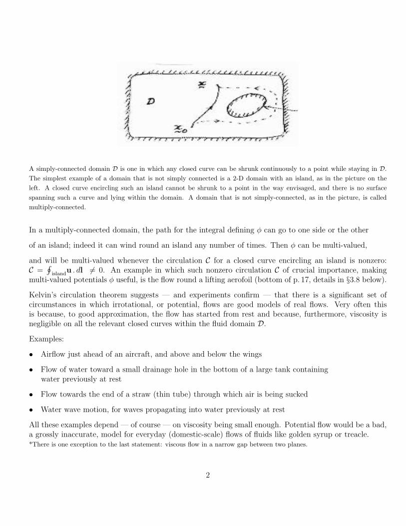
A simply-connected domain D is one in which any closed curve can be shrunk continuously to a point while staying in D.The simplest example of a domain that is not simply connected is a 2-D domain with an island, as in the picture on theleft. A closed curve encircling such an island cannot be shrunk to a point in the way envisaged, and there is no surfacespanning such a curve and lying within the domain. A domain that is not simply-connected, as in the picture, is calledmultiply-connected.

In a multiply-connected domain, the path for the integral defining φ can go to one side or the other

of an island; indeed it can wind round an island any number of times. Then φ can be multi-valued,

and will be multi-valued whenever the circulation C for a closed curve encircling an island is nonzero:C =

∮island

u . dl 6= 0. An example in which such nonzero circulation C of crucial importance, makingmulti-valued potentials φ useful, is the flow round a lifting aerofoil (bottom of p. 17, details in §3.8 below).

Kelvin’s circulation theorem suggests — and experiments confirm — that there is a significant set ofcircumstances in which irrotational, or potential, flows are good models of real flows. Very often thisis because, to good approximation, the flow has started from rest and because, furthermore, viscosity isnegligible on all the relevant closed curves within the fluid domain D.

Examples:

• Airflow just ahead of an aircraft, and above and below the wings

• Flow of water toward a small drainage hole in the bottom of a large tank containingwater previously at rest

• Flow towards the end of a straw (thin tube) through which air is being sucked

• Water wave motion, for waves propagating into water previously at rest

All these examples depend — of course — on viscosity being small enough. Potential flow would be a bad,a grossly inaccurate, model for everyday (domestic-scale) flows of fluids like golden syrup or treacle.*There is one exception to the last statement: viscous flow in a narrow gap between two planes.

2

For irrotational flow to be a good model we need ∇× F negligible in the vorticity equation

Dωωω

Dt= (ωωω.∇)u +∇× F .

where F includes, besides gravity, the force per unit mass from internal friction (viscosity).

*In the simplest case of a uniformly viscous flow under gravity or other conservative force field, the viscous contributionto F can be shown to be equal to ∇2u times a constant coefficient called the ‘kinematic viscosity’ having dimensions oflength2/time. In that case, ∇×F ∝ ∇2ωωω (which happens to be zero for potential flows — a fact that historically seems tohave caused some confusion, for perhaps a century or so, until early in the twentieth century when pioneers in aerodynamics(especially Ludwig Prandtl) saw the importance of what happens to material curves very close to boundaries, where flow ishardly ever irrotational, and began to develop the ‘boundary layer theory’ needed to understand this. For the time being,in these lectures, we can adopt the usual attitude to scientific model-making: simply adopt a set of assumptions, including,in this case, the assumption that ωωω = 0 everywhere, then ask how far the resulting model fits reality in various cases. (Forfurther discussion of, and insight into, scientific model-making as such — and such insight has great importance in today’sand tomorrow’s world — see the animated image on my home page, http://www.atmos-dynamics.damtp.cam.ac.uk/people/mem/,and associated links).*

Let us now look at some basic properties of irrotational flows.

Mass conservation ∇.u = 0 gives ∇.(∇φ) = 0, i.e.,

∇2φ = 0 ,

i.e., φ is a harmonic function, in the sense of satisfying Laplace’s equation.

The boundary condition for impermeable boundaries, also called the ‘kinematic boundary condition’, isthat

U.n = u.n = n.(∇φ) ≡ ∂φ

∂n,

where U is the velocity of points on boundary as before.*This exemplifies what is called a Neumann boundarycondition for Laplace’s equation.* If the flow is irrotational, this is the only boundary condition we need.

We can now apply techniques from Part IB Methods. For complex geometries, we can solve numerically— see Part II(a) or (b) Numerical Analysis.

§3.2 Some examples

Because φ satisfies Laplace’s equation ∇2φ = 0, we can apply all the mathematical machinery of potentialtheory, developed in 1B Methods:

A: Spherical geometry, axisymmetric flow

3

Recall the general axisymmetric solution of Laplace’s equation obtained by separation-of-variable methodsin the usual spherical polar coordinates, by trying φ = R(r) Θ(θ), etc.,

φ =∞∑n=0

{Anr

n +Bnr−(n+1)

}Pn(cos θ),

where An, Bn are arbitrary constants, Pn is the Legendre polynomial of degree n, r is the spherical radius(r2 = x2 + y2 + z2), so that z = r cos θ, and θ is the co-latitude. (Recall that P0(µ) = 1, P1(µ) = µ,P2(µ) = 3

2µ2 − 1

2, etc.)

Let us look more closely at the kinds of flows represented by the first three nontrivial terms, those withcoefficients B0, A1, and B1.

(i) all A’s, B’s zero except B0 [Notation: er = unit radial vector = x/|x| = x/r]:

φ =B0

r=B0

|x|, ⇒ u = ∇φ = −B0x

|x|3= −B0er

r2.(∗)

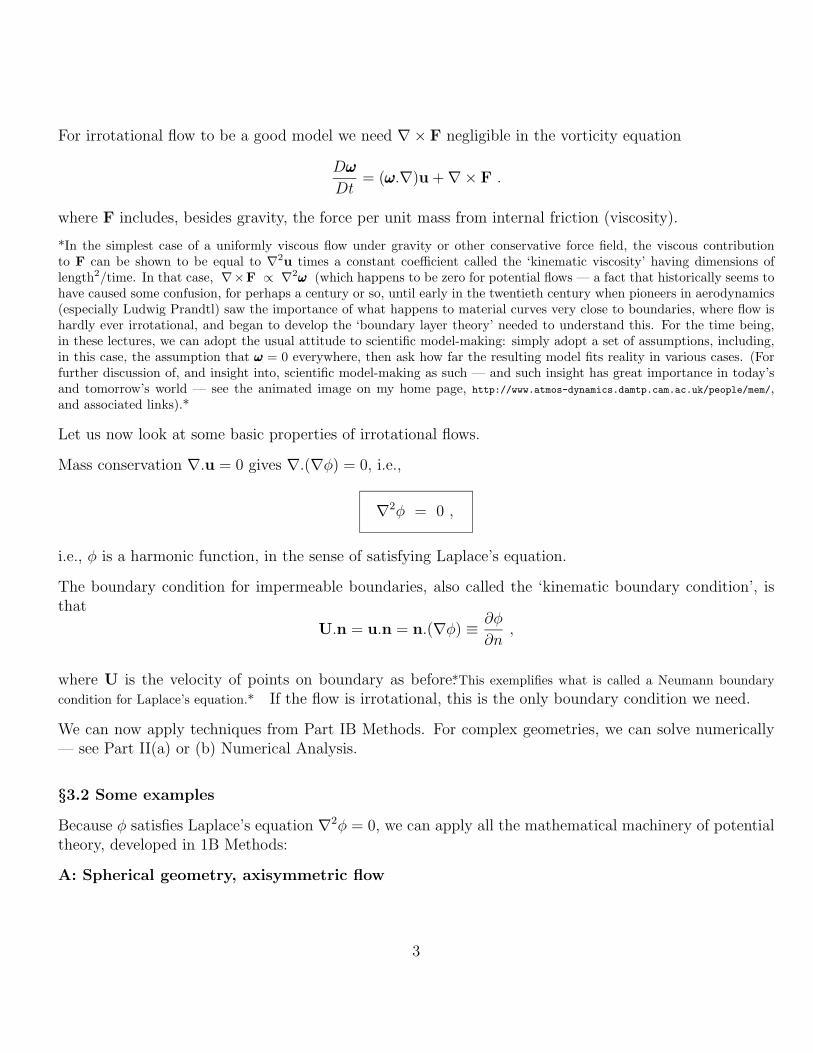
This represents source or sink flow, i.e., depending on the sign of the coefficient B0, it representsradial outflow from a point source (B0 < 0), or inflow to a point sink (B0 > 0), at the origin. Massappears or disappears, at the singularity at the origin, according as B0

<> 0. The velocity field is

radially symmetric in both cases:

source flow (B0 < 0) sink flow (B0 > 0)

Let us check that incompressibility and mass conservation are satisfied: the outward mass fluxacross any surface containing the origin should be independent of the choice of surface. For sim-plicity, take a sphere of radius R. The outward mass flux is ρ∇φ = −ρB0/R

2 per unit area, hence−(ρB0/R

2)(4πR2) in total, = −4πρB0, independent of R as expected.

(ii) all A’s, B’s zero except A1:

φ = A1r cos θ = A1z , ⇒ u = ∇φ = A1ez

4

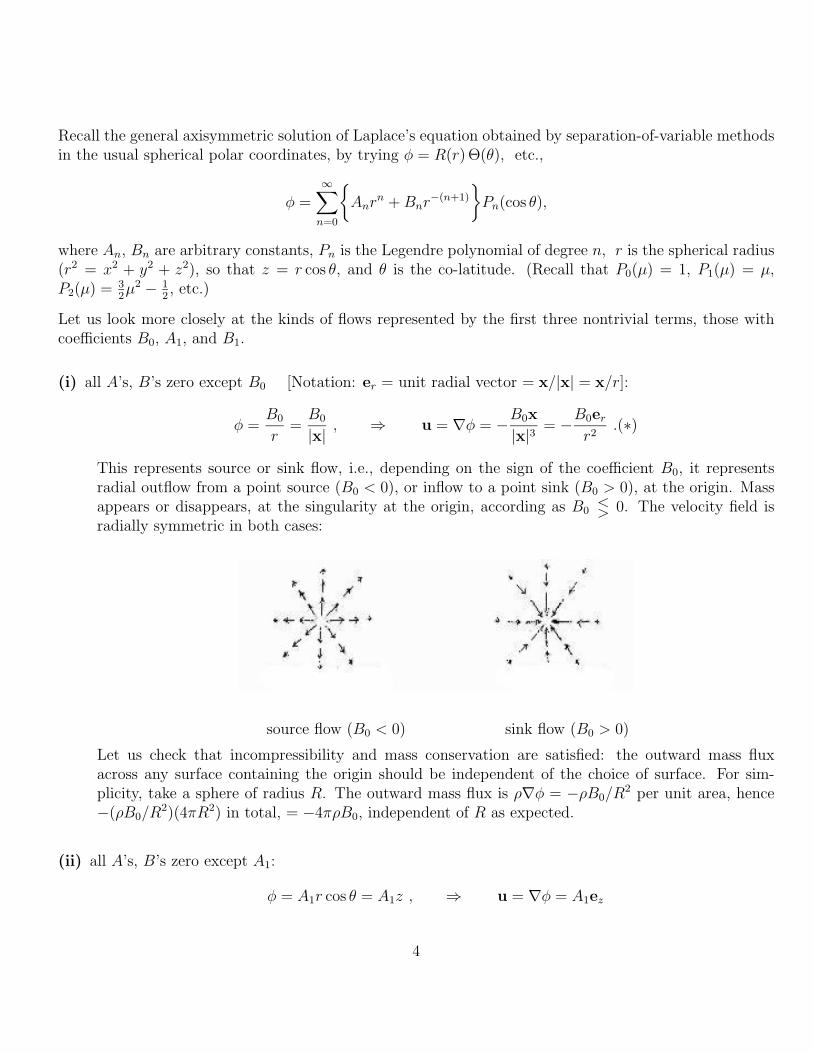
where z is the Cartesian co-ordinate parallel to the symmetry axis, and ez = (0, 0, 1) a unit axialvector. So this simply represents uniform flow in axial or z direction, a u field like this:

→ → → → → → → → → → → → → → → →→ → → → → → → → → → → → → → → →→ → → → → → → → → → → → → → → → −−−→ z

→ → → → → → → → → → → → → → → →→ → → → → → → → → → → → → → → →

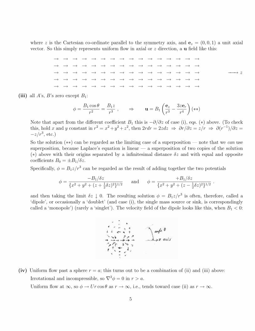
(iii) all A’s, B’s zero except B1:

φ =B1 cos θ

r2=B1z

r3, ⇒ u = B1

(ezr3− 3zer

r4

)(∗∗)

Note that apart from the different coefficient B1 this is −∂/∂z of case (i), eqs. (∗) above. (To checkthis, hold x and y constant in r2 = x2 +y2 +z2, then 2rdr = 2zdz ⇒ ∂r/∂z = z/r ⇒ ∂(r−1)/∂z =−z/r3, etc.)

So the solution (∗∗) can be regarded as the limiting case of a superposition — note that we can usesuperposition, because Laplace’s equation is linear — a superposition of two copies of the solution(∗) above with their origins separated by a infinitesimal distance δz and with equal and oppositecoefficients B0 = ±B1/δz.

Specifically, φ = B1z/r3 can be regarded as the result of adding together the two potentials

φ =−B1/δz

{x2 + y2 + (z + 12δz)2}1/2

and φ =+B1/δz

{x2 + y2 + (z − 12δz)2}1/2

.

and then taking the limit δz ↓ 0. The resulting solution φ = B1z/r3 is often, therefore, called a

‘dipole’, or occasionally a ‘doublet’ (and case (i), the single mass source or sink, is correspondinglycalled a ‘monopole’) (rarely a ‘singlet’). The velocity field of the dipole looks like this, when B1 < 0:

(iv) Uniform flow past a sphere r = a; this turns out to be a combination of (ii) and (iii) above:

Irrotational and incompressible, so ∇2φ = 0 in r > a.

Uniform flow at ∞, so φ→ Ur cos θ as r →∞, i.e., tends toward case (ii) as r →∞.

5

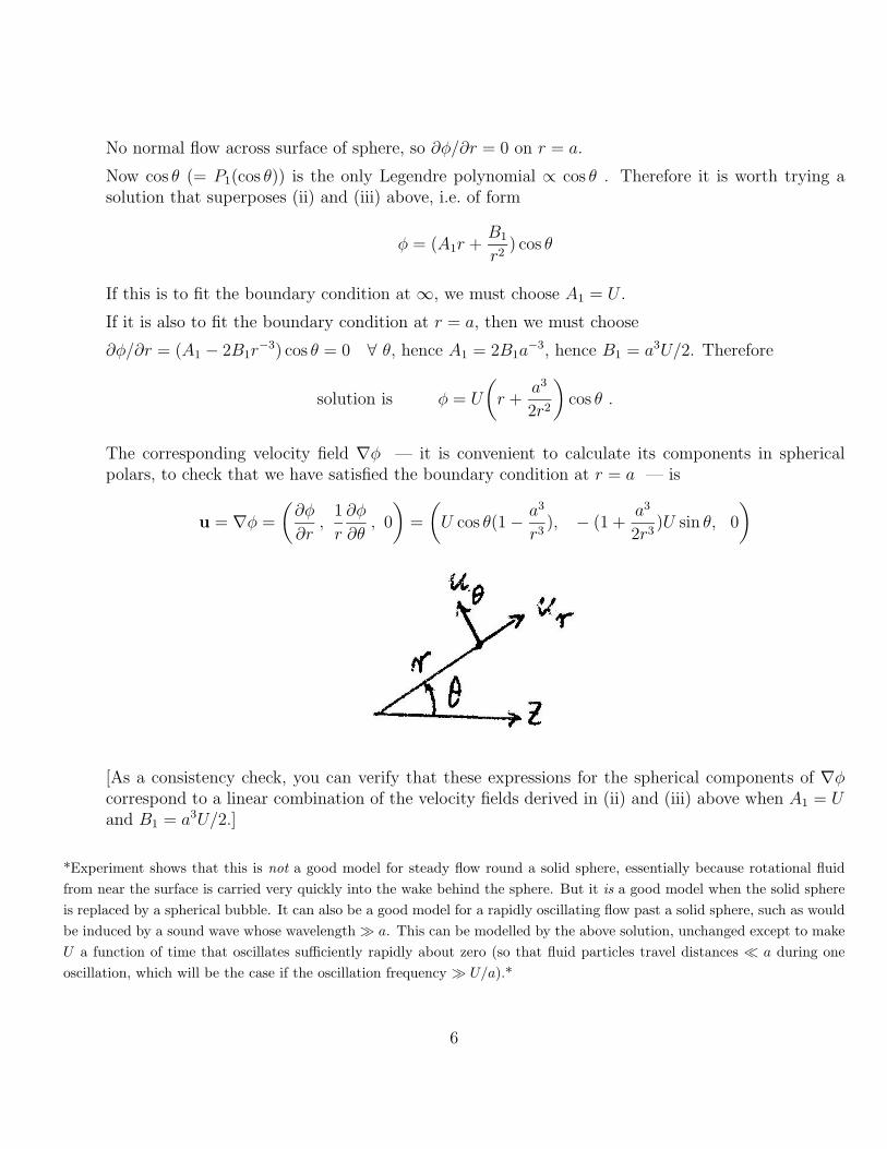
No normal flow across surface of sphere, so ∂φ/∂r = 0 on r = a.

Now cos θ (= P1(cos θ)) is the only Legendre polynomial ∝ cos θ . Therefore it is worth trying asolution that superposes (ii) and (iii) above, i.e. of form

φ = (A1r +B1

r2) cos θ

If this is to fit the boundary condition at ∞, we must choose A1 = U .

If it is also to fit the boundary condition at r = a, then we must choose

∂φ/∂r = (A1 − 2B1r−3) cos θ = 0 ∀ θ, hence A1 = 2B1a

−3, hence B1 = a3U/2. Therefore

solution is φ = U

(r +

a3

2r2

)cos θ .

The corresponding velocity field ∇φ — it is convenient to calculate its components in sphericalpolars, to check that we have satisfied the boundary condition at r = a — is

u = ∇φ =

(∂φ

∂r,

1

r

∂φ

∂θ, 0

)=

(U cos θ(1− a3

r3), − (1 +

a3

2r3)U sin θ, 0

)

[As a consistency check, you can verify that these expressions for the spherical components of ∇φcorrespond to a linear combination of the velocity fields derived in (ii) and (iii) above when A1 = Uand B1 = a3U/2.]

*Experiment shows that this is not a good model for steady flow round a solid sphere, essentially because rotational fluidfrom near the surface is carried very quickly into the wake behind the sphere. But it is a good model when the solid sphereis replaced by a spherical bubble. It can also be a good model for a rapidly oscillating flow past a solid sphere, such as wouldbe induced by a sound wave whose wavelength � a. This can be modelled by the above solution, unchanged except to makeU a function of time that oscillates sufficiently rapidly about zero (so that fluid particles travel distances � a during oneoscillation, which will be the case if the oscillation frequency � U/a).*

6

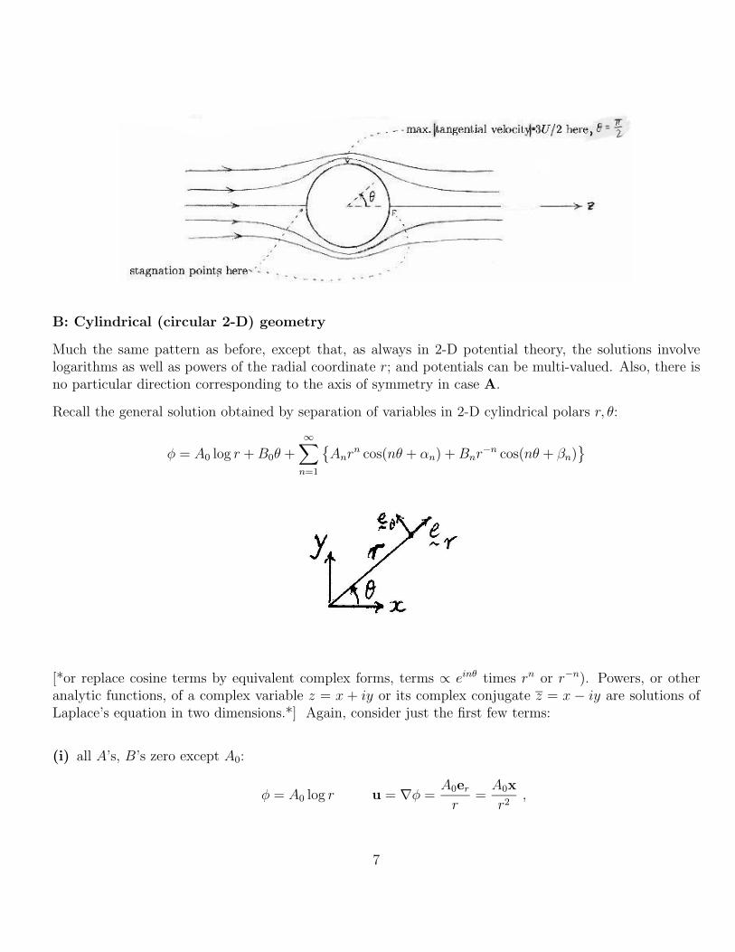
B: Cylindrical (circular 2-D) geometry

Much the same pattern as before, except that, as always in 2-D potential theory, the solutions involvelogarithms as well as powers of the radial coordinate r; and potentials can be multi-valued. Also, there isno particular direction corresponding to the axis of symmetry in case A.

Recall the general solution obtained by separation of variables in 2-D cylindrical polars r, θ:

φ = A0 log r +B0θ +∞∑n=1

{Anr

n cos(nθ + αn) +Bnr−n cos(nθ + βn)

}

[*or replace cosine terms by equivalent complex forms, terms ∝ einθ times rn or r−n). Powers, or otheranalytic functions, of a complex variable z = x + iy or its complex conjugate z = x − iy are solutions ofLaplace’s equation in two dimensions.*] Again, consider just the first few terms:

(i) all A’s, B’s zero except A0:

φ = A0 log r u = ∇φ =A0err

=A0x

r2,

7

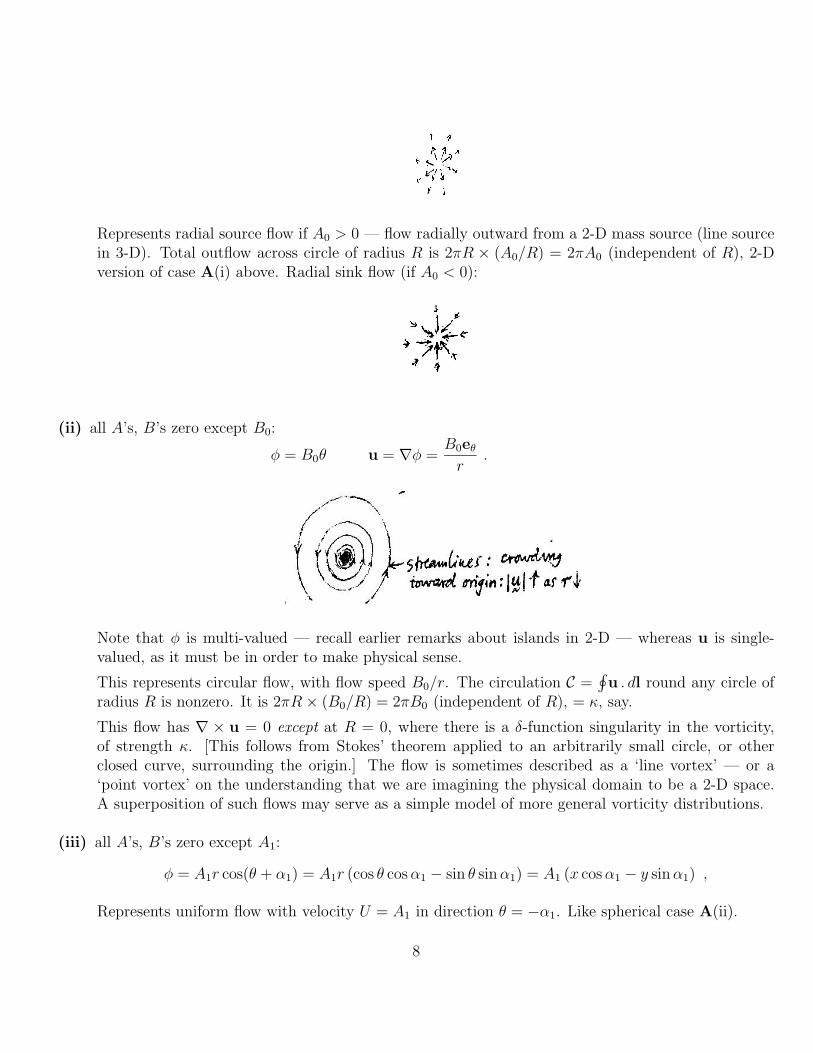
Represents radial source flow if A0 > 0 — flow radially outward from a 2-D mass source (line sourcein 3-D). Total outflow across circle of radius R is 2πR × (A0/R) = 2πA0 (independent of R), 2-Dversion of case A(i) above. Radial sink flow (if A0 < 0):

(ii) all A’s, B’s zero except B0:

φ = B0θ u = ∇φ =B0eθr

.

Note that φ is multi-valued — recall earlier remarks about islands in 2-D — whereas u is single-valued, as it must be in order to make physical sense.

This represents circular flow, with flow speed B0/r. The circulation C =∮

u . dl round any circle ofradius R is nonzero. It is 2πR× (B0/R) = 2πB0 (independent of R), = κ, say.

This flow has ∇ × u = 0 except at R = 0, where there is a δ-function singularity in the vorticity,of strength κ. [This follows from Stokes’ theorem applied to an arbitrarily small circle, or otherclosed curve, surrounding the origin.] The flow is sometimes described as a ‘line vortex’ — or a‘point vortex’ on the understanding that we are imagining the physical domain to be a 2-D space.A superposition of such flows may serve as a simple model of more general vorticity distributions.

(iii) all A’s, B’s zero except A1:

φ = A1r cos(θ + α1) = A1r (cos θ cosα1 − sin θ sinα1) = A1 (x cosα1 − y sinα1) ,

Represents uniform flow with velocity U = A1 in direction θ = −α1. Like spherical case A(ii).

8

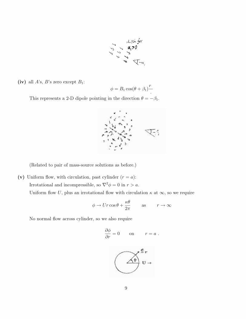
(iv) all A’s, B’s zero except B1:

φ = B1 cos(θ + β1)r

.

This represents a 2-D dipole pointing in the direction θ = −β1.

(Related to pair of mass-source solutions as before.)

(v) Uniform flow, with circulation, past cylinder (r = a):

Irrotational and incompressible, so ∇2φ = 0 in r > a.

Uniform flow U , plus an irrotational flow with circulation κ at ∞, so we require

φ→ Ur cos θ +κθ

2πas r →∞

No normal flow across cylinder, so we also require

∂φ

∂r= 0 on r = a .

9

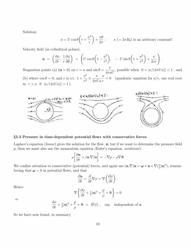
Solution:

φ = U cos θ

(r +

a2

r

)+κθ

2π; κ (= 2πB0) is an arbitrary constant!

Velocity field (in cylindrical polars):

u =

(∂φ

∂r,

1

r

∂φ

∂θ

)=

(U cos θ

(1− a2

r2

), − U sin θ

(1 +

a2

r2

)+

κ

2πr

).

Stagnation points (a) (u = 0) on r = a and sin θ =κ

4πaU, possible when 0 < |κ/(4πUa)| < 1 , and

(b) where cos θ = 0, and r is s.t. 1 +a2

r2∓ κ

2πUa

a

r= 0 (quadratic equation for a/r, one real root

in r > a if |κ/(4πUa)| > 1 ).

§3.3 Pressure in time-dependent potential flows with conservative forces

Laplace’s equation (linear) gives the solution for the flow, u; but if we want to determine the pressure fieldp, then we must also use the momentum equation (Euler’s equation, nonlinear):

ρ

[∂u

∂t+ (u.∇)u

]= −∇p− ρ∇Φ

We confine attention to conservative (potential) forces, and again use (u.∇)u = ωωω×u +∇(12|u|2), remem-

bering that ωωω = 0 in potential flows, and that

∂u

∂t=

∂

∂t∇φ = ∇

(∂φ

∂t

).

Hence

∇{∂φ

∂t+ 1

2|u|2 +

p

ρ+ Φ

}= 0

⇒∂φ

∂t+ 1

2|u|2 +

p

ρ+ Φ = H(t) , say, independent of x.

So we have now found, in summary,

10

Two forms of Bernoulli’s theorem

both applying to the flow of an inviscid, incompressible fluid under conservative (potential) forces −∇Φper unit mass, and both being corollaries of the momentum equation written as

∂u

∂t+ 1

2∇(|u|2)

+ ωωω × u = − 1

ρ∇p+∇Φ .

The two forms, deduced in §2.4 and just above, respectively say that:

IF the flow is

steady, i.e.∂u

∂t= 0, irrotational, i.e. ∇× u = 0,

then the quantity

H = 12|u|2 +

p

ρ+ Φ H =

∂φ

∂t+ 1

2|u|2 +

p

ρ+ Φ

obeys

u .∇(12|u|2 +

p

ρ+ Φ) = 0 ∇

(∂φ

∂t+ 1

2|u|2 +

p

ρ+ Φ

)= 0

and hence12|u|2 +

p

ρ+ Φ = H = constant on

∂φ

∂t+ 1

2|u|2 +

p

ρ+ Φ = H(t), independent

streamlines of spatial position x

We may also summarize, and slightly generalize, the ways of representing the velocity field in variouscircumstances, as follows:

Stream function and velocity potential (§§1.8 & 3.1)

IF the flow isincompressible, i.e. ∇ .u = 0, irrotational, i.e. ∇× u = 0,

then there exists*a vector potential A a scalar potential φ

with u = ∇×A * with u = +∇φ

*In 2-D (or axisymmetric) flow A hasonly one component, from which we (φ being called the velocity potential)define* a stream function ψ (or Ψ)

11

u ⊥ ∇ψ (or ∇Ψ) so u ‖ +∇φψ (or Ψ) is constant on streamlines

In a multiply connected domain in 2-D:ψ may be multi-valued if ∃ islands/holes φ may be multi-valued if ∃ islands/holes

with net outflow:∮

u .n ds 6= 0 with net circulation:∮

u . dl 6= 0

§3.4 Applications of irrotational, time-dependent Bernoulli

Inviscid, irrotational models can give useful insight into certain kinds of unsteady fluid behaviour and theirtimescales, relevant to laboratory and industrial fluid systems. The simplest examples include acceleratingflows in tubes:

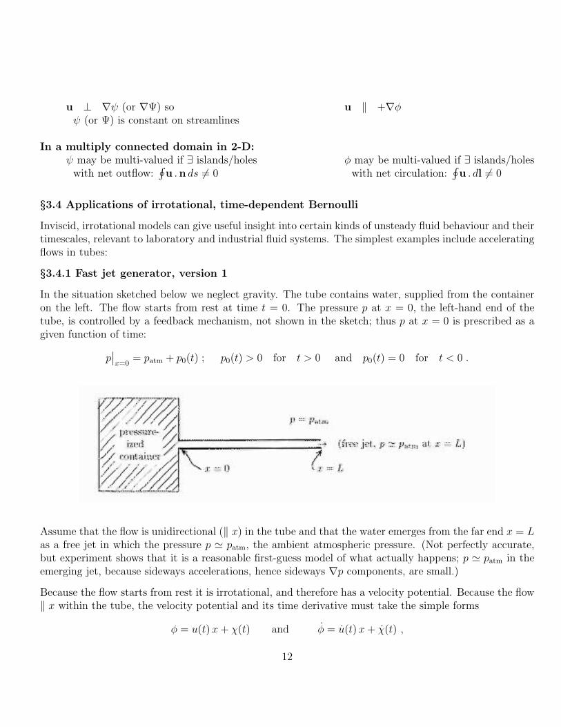
§3.4.1 Fast jet generator, version 1

In the situation sketched below we neglect gravity. The tube contains water, supplied from the containeron the left. The flow starts from rest at time t = 0. The pressure p at x = 0, the left-hand end of thetube, is controlled by a feedback mechanism, not shown in the sketch; thus p at x = 0 is prescribed as agiven function of time:

p∣∣x=0

= patm + p0(t) ; p0(t) > 0 for t > 0 and p0(t) = 0 for t < 0 .

Assume that the flow is unidirectional (‖ x) in the tube and that the water emerges from the far end x = Las a free jet in which the pressure p ' patm, the ambient atmospheric pressure. (Not perfectly accurate,but experiment shows that it is a reasonable first-guess model of what actually happens; p ' patm in theemerging jet, because sideways accelerations, hence sideways ∇p components, are small.)

Because the flow starts from rest it is irrotational, and therefore has a velocity potential. Because the flow‖ x within the tube, the velocity potential and its time derivative must take the simple forms

φ = u(t)x+ χ(t) and φ = u(t)x+ χ(t) ,

12

where χ(t) is an arbitrary function of time t alone, and where u is the flow velocity along the tube. Notethat φ cannot depend on y or z; otherwise the flow not ‖ x. So u cannot depend on y or z either; nor canu depend on x, otherwise ∇2φ 6= 0 (∇.u 6= 0, mass not conserved).

Apply time-dependent Bernoulli: H constant along tube, H∣∣x>0

= H∣∣x=0

= constant; so

u x+ χ+ 12u2 +

p

ρ= u 0 + χ+ 1

2u2 +

p0(t)

ρ.

Notice the implication that p = p(x, t) and moreover that −∇p = (ρu, 0, 0) . (Pressure varies linearlywith x; pressure gradient is uniform along the tube, as it has to be because fluid acceleration is uniformalong the tube.) Taking p = 0 at x = L, we have (with several terms cancelling or vanishing)

u L +0

ρ= u 0 +

p0(t)

ρ,

so

u =p0(t)

ρL, ⇒ u =

1

ρL

∫ t

0

p0(t′) dt′ .

E.g. if p0 = positive constant for t > 0, then

u =p0

ρLt .

So the flow keeps accelerating as long as this model remains applicable, i.e., as long as friction (viscosity)remains unimportant and as long as the excess pressure p0 is maintained (by the pressurized container andthe assumed control mechanism).

Notice that χ(t) has disappeared from the problem. Indeed we could have taken χ(t) = 0 w.l.o.g. at theoutset, on the grounds that only ∇φ is of physical interest and that ∇χ(t) = 0. This would have changedthe value of H, but not the thing that matters — the constancy of H.

§3.4.2 Fast jet generator, version 2

Same problem as before, except that pressure now controlled via force on piston to be patm +p0(t) here; sopressure here (x = 0) is now unknown:

13

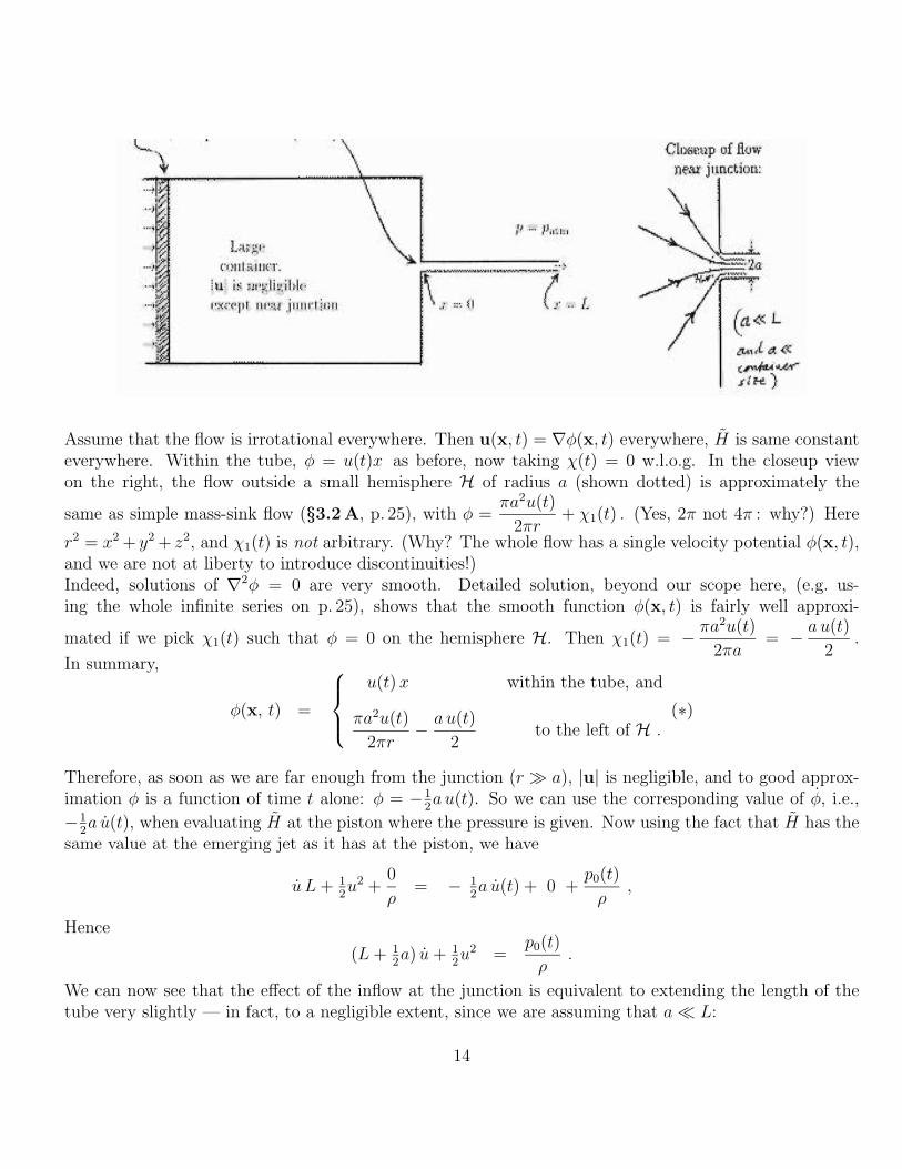
Assume that the flow is irrotational everywhere. Then u(x, t) = ∇φ(x, t) everywhere, H is same constanteverywhere. Within the tube, φ = u(t)x as before, now taking χ(t) = 0 w.l.o.g. In the closeup viewon the right, the flow outside a small hemisphere H of radius a (shown dotted) is approximately the

same as simple mass-sink flow (§3.2 A, p. 25), with φ =πa2u(t)

2πr+ χ1(t) . (Yes, 2π not 4π : why?) Here

r2 = x2 + y2 + z2, and χ1(t) is not arbitrary. (Why? The whole flow has a single velocity potential φ(x, t),and we are not at liberty to introduce discontinuities!)Indeed, solutions of ∇2φ = 0 are very smooth. Detailed solution, beyond our scope here, (e.g. us-ing the whole infinite series on p. 25), shows that the smooth function φ(x, t) is fairly well approxi-

mated if we pick χ1(t) such that φ = 0 on the hemisphere H. Then χ1(t) = − πa2u(t)

2πa= − a u(t)

2.

In summary,

φ(x, t) =

u(t)x within the tube, and

πa2u(t)

2πr− a u(t)

2to the left of H .

(∗)

Therefore, as soon as we are far enough from the junction (r � a), |u| is negligible, and to good approx-imation φ is a function of time t alone: φ = −1

2a u(t). So we can use the corresponding value of φ, i.e.,

−12a u(t), when evaluating H at the piston where the pressure is given. Now using the fact that H has the

same value at the emerging jet as it has at the piston, we have

u L+ 12u2 +

0

ρ= − 1

2a u(t) + 0 +

p0(t)

ρ,

Hence

(L+ 12a) u+ 1

2u2 =

p0(t)

ρ.

We can now see that the effect of the inflow at the junction is equivalent to extending the length of thetube very slightly — in fact, to a negligible extent, since we are assuming that a� L:

14

L u+ 12u2 =

p0(t)

ρ.(∗∗)

(*We can also see that detailed, more accurate solution of ∇2φ = 0 for the inflow near the junction can hardly change

the picture: the factor 12 multiplying a u will be replaced by a slightly different numerical coefficient, but this does not

alter the negligible order of magnitude. Similar considerations govern the oscillatory flow near the end of an organ pipe: thepipe behaves acoustically as if it were slightly longer than it looks, by an amount roughly of the order of the pipe radius.Acousticians call this an ‘end correction’ to the length of the pipe.*)

Now (∗∗) is a nonlinear first-order ODE for the function u(t), to be solved with initial condition u(0) = 0.For general p0(t) it can be solved only by numerical methods, but it can be solved analytically in the casewhere p0 = positive constant for t > 0. It is then a separable first-order ODE. Before solving it, let us tidyit up by defining u0, U(T ) and T by

u0 =√

2p0/ρ , > 0 for t > 0 , T = u0t/2L , and U(t) = u(t)/u0 .

Then (∗∗) becomesdU

dT= 1− U2 ,

to be solved with initial condition U(0) = 0.

The constants u0 and 2L/u0 can reasonably be called the natural velocity scale and timescale for thisproblem.

Solving by separation of variables then partial fractions, we have∫dT =

∫dU

1− U2=

∫dU

2

(1

1 + U+

1

1− U

)= 1

2log

(1 + U

1− U

)+ const. ;

so1 + U

1− U∝ const.× e2T ; initial conditions⇒ const. of proportionality = 1 ;

therefore

U =e2T − 1

e2T + 1= tanh T ;

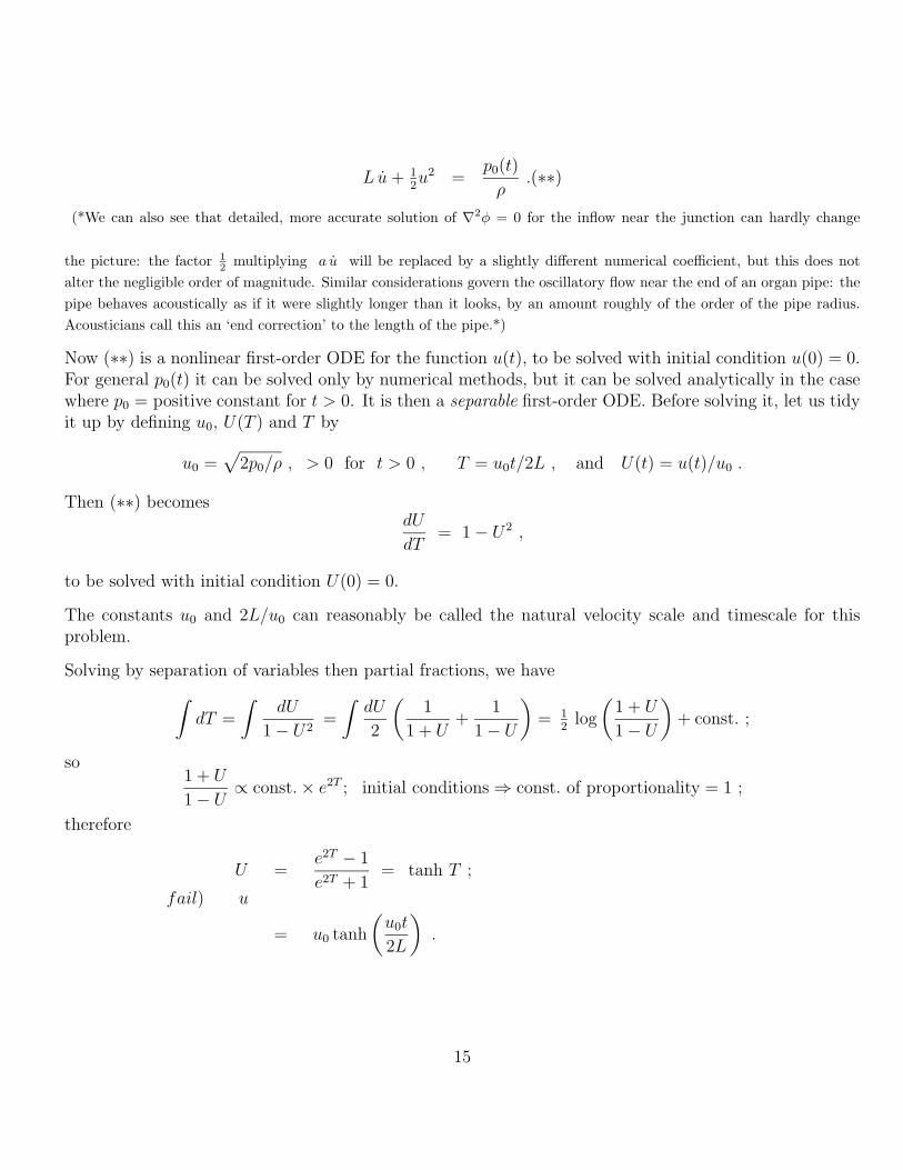
fail) u

= u0 tanh

(u0t

2L

).

15

So this second version of the jet problem is very different from the first version! Even in an frictionless(inviscid) model, the nonlinear term 1

2u2 in the ODE (∗∗) limits the jet speed to a finite maximum value

u0, determined entirely by the imposed pressure p0.

There is a similar problem in which gravity is important, and acts in place of the large piston. The waterin the (large) container has a free upper surface at vertical distance h, say, above the (horizontal) tube.

The answer is the same except that u0 =√

2gh instead of√

2p0/ρ (sheet 2 Q7).

§3.4.3 Inviscid manometer oscillations

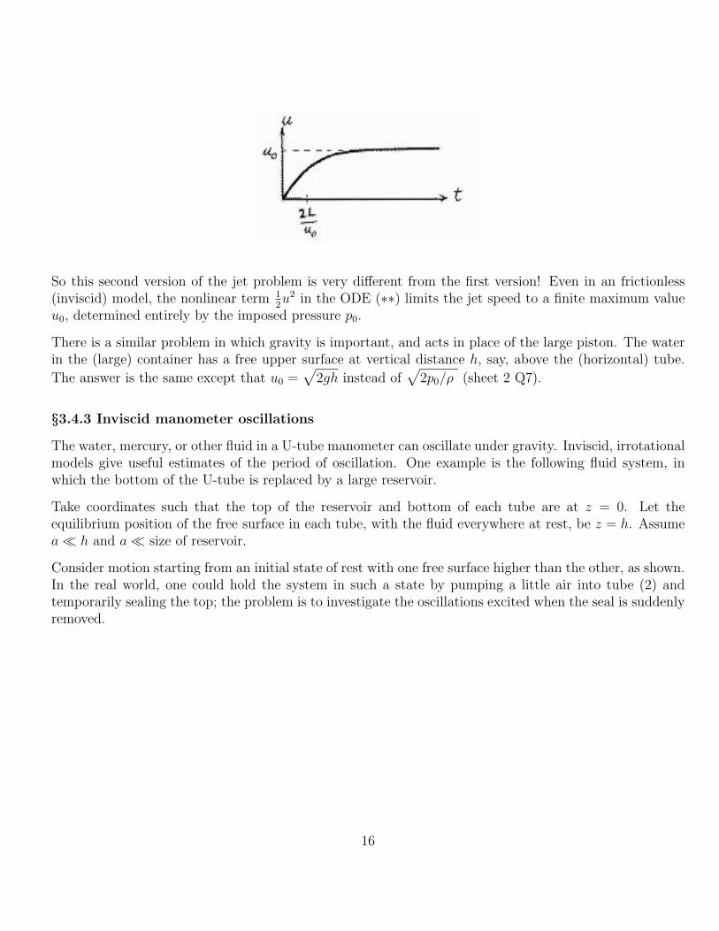
The water, mercury, or other fluid in a U-tube manometer can oscillate under gravity. Inviscid, irrotationalmodels give useful estimates of the period of oscillation. One example is the following fluid system, inwhich the bottom of the U-tube is replaced by a large reservoir.

Take coordinates such that the top of the reservoir and bottom of each tube are at z = 0. Let theequilibrium position of the free surface in each tube, with the fluid everywhere at rest, be z = h. Assumea� h and a� size of reservoir.

Consider motion starting from an initial state of rest with one free surface higher than the other, as shown.In the real world, one could hold the system in such a state by pumping a little air into tube (2) andtemporarily sealing the top; the problem is to investigate the oscillations excited when the seal is suddenlyremoved.

16

Once again, we argue that the flow starts from rest, hence remains irrotational (in this inviscid fluid model),hence may be described by a velocity potential φ. Just as before, we take the flow to be uniform withineach tube, u = (0, 0, w), a function of time alone. Mass conservation requires that, in the first tube, say,w = ζ1 where the dot denotes the time derivative, and likewise in the second tube, where w = ζ2 = −ζ1.The last relation, ζ2 = −ζ1, follows from overall mass conservation for the entire, rigidly bounded, system.

In tube (1), uniform flow u = (0, 0, ζ1) ⇒ φ = φ1(z, t) = ζ1(t)z;

In tube (2), uniform flow (0, 0, ζ2) ⇒ φ = φ2(z, t) = ζ2(t)z + χ1(t) .

The additive function of time alone makes no difference to the velocity field, but as before is relevant tothe Bernoulli quantity H, and so needs to be included — though we shall find, in the same way as before,that it is negligible. (Once again, we must remember, there is a single, and in this problem single-valued,potential function φ(x, t) — single-valued because the fluid domain is simply connected — describing theflow in the whole system. The above expressions merely give local approximations to that single function,applicable only within tube (1) or tube (2).

Now apply the constancy of H:

H =∂φ

∂t+ 1

2|u|2 +

p

ρ+ gz is spatially uniform (though possibly time-dependent).

17

In particular, H must have the same values at the two free surfaces, i.e. at z = h + ζ1 in tube (1) andz = h+ ζ2 in tube (2). Therefore

(ζ1z + 1

2ζ2

1 +patm

ρ+ gz

)∣∣∣∣z=h+ζ1

=

(ζ2z + χ1 + 1

2ζ2

2 +patm

ρ+ gz

)∣∣∣∣z=h+ζ2

⇒ζ1(h+ ζ1) + 1

2ζ2

1 + gh+ gζ1 = ζ2(h+ ζ2) + 12ζ2

2 + gh+ gζ2 + χ1 ,

As already noted, ζ1 + ζ2 = 0, hence ζ1ζ1 = ζ2ζ2 and ζ21 = ζ2

2 . Hence all the nonlinear terms cancel:

ζ1h+ gζ1 = 12χ1 .(∗)

By considering the flow near the junctions of the tubes with the reservoir, we can show, just as before, thatthe right-hand side is small of order a/h relative to the first term on the left-hand side, and can thereforebe neglected to a first approximation.

The equation (∗), with its r.h.s. replaced by zero, implies that the oscillations are sinusoidal of period2π(h/g)1/2; e.g. 1 second when h = 25 cm and g = 980 cm s−2.

Note that there is no formal restriction to small amplitude, because of the cancellation of the nonlinearterms. (That cancellation, however, depends on our assumption that the two tubes have the same cross-sectional area. Ex. Sheet 2 Q8 is an example where this does not apply, and where the nonlinearities aretherefore significant, just as they are in version 2 of the jet problem.)

What has just been shown can be thought of in the following way. For the purpose of understanding themanometer oscillations, we may pretend that tubes (1) and (2) are joined not by an enormous reservoir,but — surprising, isn’t it? — by a very short extra length of tubing, which the above approximate analysis(p. 32) says has total length 1

2a (if it has radius a). More refined analyses say it has total length a times a

modest numerical factor, not quite 12. The main conclusion, which relies only on the assumption a � h,

is unaffected.

(*But if the joining tube is constricted to a cross-sectional area � πa2 then this adds significant inertia, hence equivalent tolonger joining tube of radius a; cf. trumpet mouthpiece.*)

*More refined analyses (which again can be found in acoustics textbooks under the heading ‘end corrections’) show thatequation (∗) and its refinements is still linear. The velocity squared terms in the Bernoulli quantity H still cancel betweenthe two regions where the tube flows merges into source or sink flow. Again, this cancellation holds only if the geometries ofthe two tubes and their outlets are the same; otherwise, if the tube geometries differ from each other, the nonlinear termswon’t cancel and the theory will then apply to small oscillations only. For real fluids, there are additional reasons why thetheory does not apply accurately at large amplitude (flow separation near the tube outlets, producing eddying, rotationalflow), though it still gives a correct idea of the timescale of the oscillations.*

§3.4.4 Bubbles and cavities: oscillations and collapse

18

This is another practically important case of unsteady flow where inviscid, irrotational fluid models areuseful, and indeed quite accurate in some circumstances. You have probably heard the musical notes,the plink, plonk sounds, that typically occur when water drips into a tank. These are due to the kind ofbubble oscillations we consider here. The collapse of cavities, temporary bubbles with near-zero interiorpressure, is an important consideration in the design of technologies that use high-energy liquid flow, e.g.in ship propeller design. Gravity is negligible in all these problems; and irrotational fluid models capturemuch of what happens.

*Such collapse can produce extraordinary concentrations of energy, and if it occurs near boundaries it can cause significantdamage to the boundary material. In certain other cases (not near boundaries), local energy densities can reach such highvalues that atoms near the origin are excited and give off photons — a phenomenon called ‘sonoluminescence’. For the lateston this, see Nature 409, 782, in the Human Genome Issue of 15 February 2001.*

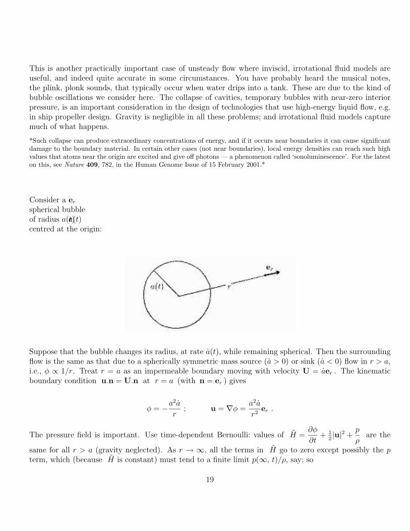
Consider a erspherical bubbleof radius a(t)a(t)rcentred at the origin:

Suppose that the bubble changes its radius, at rate a(t), while remaining spherical. Then the surroundingflow is the same as that due to a spherically symmetric mass source (a > 0) or sink (a < 0) flow in r > a,i.e., φ ∝ 1/r. Treat r = a as an impermeable boundary moving with velocity U = aer . The kinematicboundary condition u.n = U.n at r = a (with n = er ) gives

φ = −a2a

r; u = ∇φ =

a2a

r2er .

The pressure field is important. Use time-dependent Bernoulli: values of H =∂φ

∂t+ 1

2|u|2 +

p

ρare the

same for all r > a (gravity neglected). As r → ∞, all the terms in H go to zero except possibly the pterm, which (because H is constant) must tend to a finite limit p(∞, t)/ρ, say; so

19

∂

∂t

(−a

2a

r

)+a4a2

2r4+p(r, t)

ρ=

p(∞, t)ρ

(Remember, ∂/∂t has x, hence r, constant:) first term = −a2a

r− 2aa2

r

⇒ a2a

r+

(4a

r− a4

r4

)a2

2=

p(r, t)

ρ− p(∞, t)

ρ.

In particular, at r = a+ (i.e. just within the incompressible fluid, just outside the bubble; i.e. in the limitas r ↓ a through values > a),

aa+ 32a2 =

p(a+, t)

ρ− p(∞, t)

ρ.(•)

(The pressure p(a−, t) just inside the bubble can differ from that just outside, p(a+, t), because of surfacetension.)

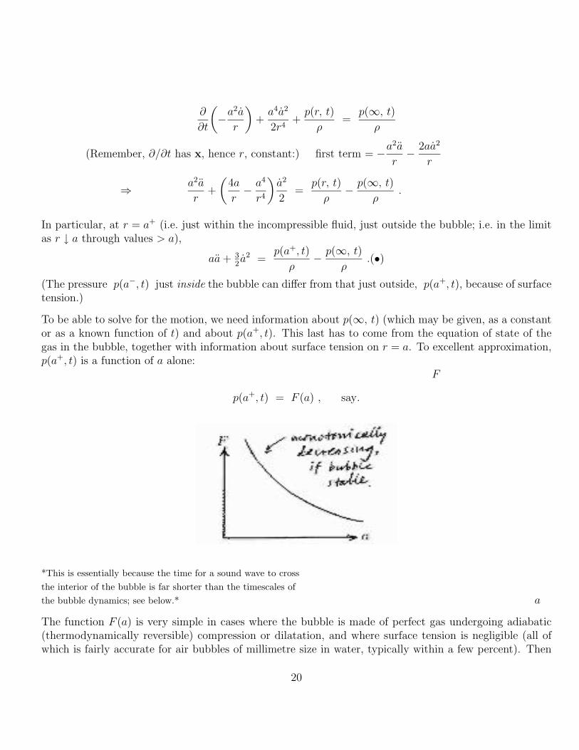
To be able to solve for the motion, we need information about p(∞, t) (which may be given, as a constantor as a known function of t) and about p(a+, t). This last has to come from the equation of state of thegas in the bubble, together with information about surface tension on r = a. To excellent approximation,p(a+, t) is a function of a alone:

F

p(a+, t) = F (a) , say.

*This is essentially because the time for a sound wave to crossthe interior of the bubble is far shorter than the timescales ofthe bubble dynamics; see below.* a

The function F (a) is very simple in cases where the bubble is made of perfect gas undergoing adiabatic(thermodynamically reversible) compression or dilatation, and where surface tension is negligible (all ofwhich is fairly accurate for air bubbles of millimetre size in water, typically within a few percent). Then

20

p(a+, t) = p(a−, t) ∝ (bubble volume)−γ ∝ (a3)−γ ∝ a−3γ, where γ is the ratio of specific heats. For airunder ordinary conditions,

γ = 7/5 = 1.4 to good approximation ,

with fractional error a percent or so. (You can take this on faith, or check it out in standard physicstextbooks.) So in all such cases

F (a) = p0

(a0

a

)3γ

, (• • •)

where p0 is the pressure in the bubble when it has radius a0.

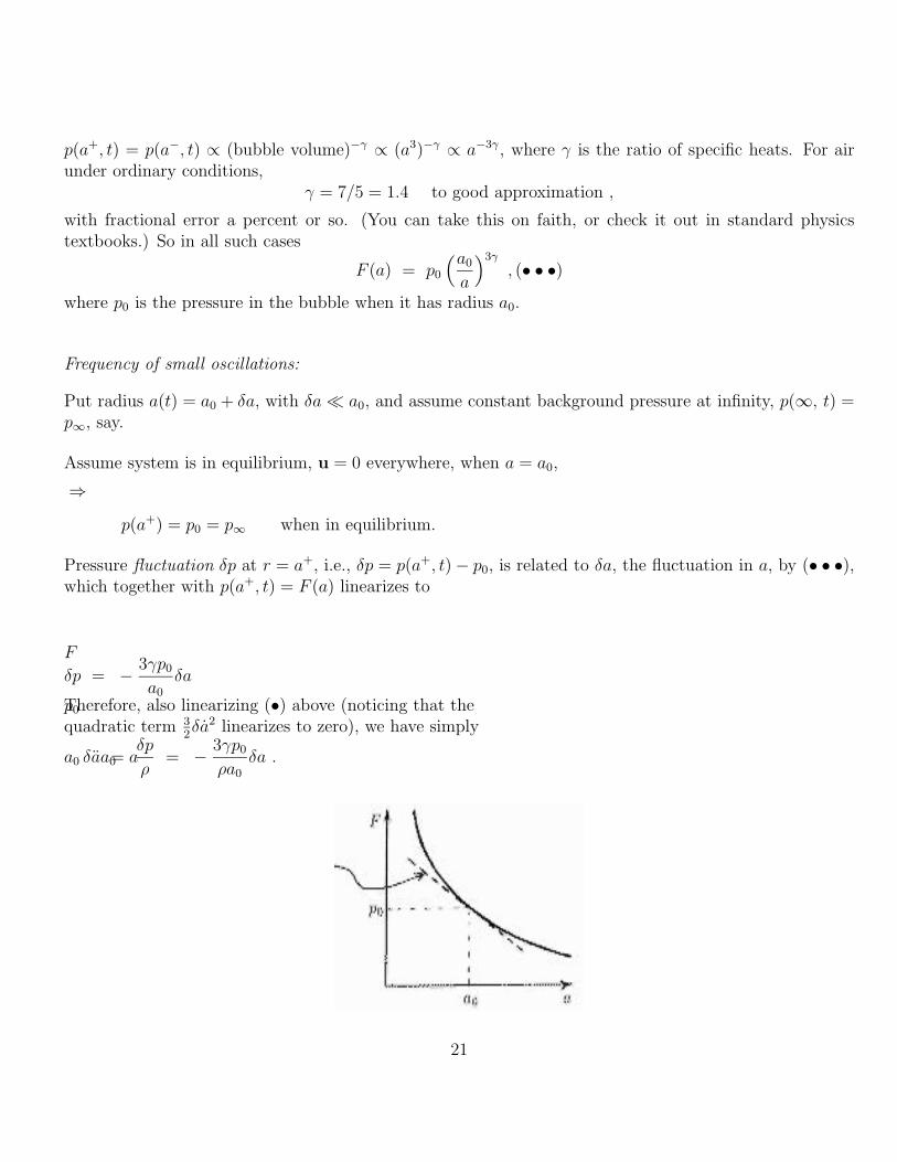
Frequency of small oscillations:

Put radius a(t) = a0 + δa, with δa� a0, and assume constant background pressure at infinity, p(∞, t) =p∞, say.

Assume system is in equilibrium, u = 0 everywhere, when a = a0,

⇒

p(a+) = p0 = p∞ when in equilibrium.

Pressure fluctuation δp at r = a+, i.e., δp = p(a+, t)− p0, is related to δa, the fluctuation in a, by (• • •),which together with p(a+, t) = F (a) linearizes to

F

δp = − 3γp0

a0

δa

Therefore, also linearizing (•) above (noticing that thep0

quadratic term 32δa2 linearizes to zero), we have simply

a0 δa =δp

ρ= − 3γp0

ρa0

δa .a0 a

21

This represents simple harmonic motion δa(t) ∝ sin(σt+ const.) with (radian) frequency

σ =

√3γp0

ρa20

.

Putting in typical numbers for air bubbles in water, under ordinary conditions (p0 = 105Pa, ρ = 103 kg m−3)we find that the frequency in hertz or cycles per second, i.e. σ/2π, ≈ 650 Hz cm/2a0 = 6.5 kHz mm/2a0.E.g. to get 1 kHz, the pitch of the radio time-pips, need a0 to be about 3.3 mm.

*We can now check, in this case, our original assumption that the time a0/cair for a sound wave to cross the bubble is farshorter than the bubble oscillation timescale σ−1. The sound speed in air is, under ordinary conditions, cair =

√(γp0/ρair) ≈

340ms−1, ρair being the air density, ∼ 10−3ρ, where ρ = density of water, 103 kg m−3 = 1 tonne/m3. We can now rewritethe formula for σ as (cair/a0)

√(3ρair/ρ), which evidently � (cair/a0), as assumed.*

To analyze the collapse problem, and other nonlinear problems, we now need to develop the general theorya little further:

Energy relation: Notice the pattern of time derivatives on l.h.s. (•). This suggests further simplificationto a single term ∝ a −1(d/dt)(a2an) for some power n; and n = 3 does the trick: a −1(d/dt)(a2a3) =2aa3 + 3a2a2 = 2a2(aa+ 3

2a2), so we have, multiplying both sides by a2a,

d

dt

(12a3a2

)= a2a

(p(a+, t)

ρ− p(∞, t)

ρ

).(••)

This is the energy equation for the fluid in r > a. We might have guessed this from the extra factor a;multiplying (•) by a2a is a bit like its counterpart in Newtonian particle dynamics, i.e., scalarly multiplyingNewton’s law of motion mx = ... by x to get (d/dt)

(12m|x|2

)= ..., the equation for the rate of change of

kinetic energy. We can check this out for the fluid problem by calculating the total kinetic energy K offlow in r > a, i.e. the volume integral of 1

2ρ|u|2:

K =

∫ ∞a

12ρ|u|2 4πr2 dr

=

∫ ∞a

12ρ

(a2a

r2

)2

4π r2 dr = 4πρ 12a4a2

∫ ∞a

dr

r2

= 4πρ 12a3a2 .

Integral is convergent and K is finite! Its rate of change K must equal the rate of working by the pressureforces on the fluid in r > a. The force per unit area exerted by the bubble on the surrounding fluid isp(a+, t); the rate of working of that force is a p(a+, t) per unit area, which sums to 4πa2a p(a+, t) for thewhole bubble. Similarly, the rate of working by the fluid in r < R, say, on the fluid beyond, in r > R, is

4πR2

(a2a

R2

)p(R, t) → 4πa2a p(∞, t) as R→∞ .

22

So the net rate of working on the whole fluid is 4πa2a{p(a+, t) − p(∞, t)

}. This must be equal to K,

which is what (••) says, after multiplying it by 4πρ. (Notice that, in this model, strict incompressibilityhas the peculiar consequence that nonzero work is done ‘at infinity’.)

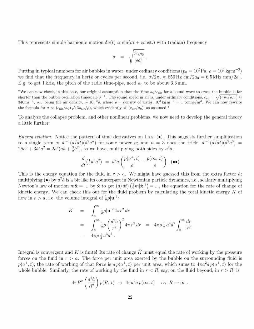
Pressure field in r > a: If we know a(t) and p(∞, t) then p(r, t) is determined by the equation displayedbefore (•). Alternatively, we can eliminate a from that equation, using (•) itself, to give

p(r, t)− p(∞, t) =

(p(a+, t)− p(∞, t)

)a

r+ 1

2ρ a2

(a

r− a4

r4

).(• • • •)

The term ∝ a2 is always positive (because r > a).(ar− a4

r4

)This is helpful in understanding the collapseproblem, to be considered next:

Collapse of cavity: A cavity is a bubble with very small interior pressures, usually formed as a resultof ‘cavitation’ in high-energy flows of liquids around convex solid boundaries, where relative flow speedscan become large and pressures low, as suggested by Bernoulli’s theorem, even to the point of becomingnegative. The classic case is that of ships’ propellers.

Liquids under ordinary conditions cannot withstand tension, i.e. negative pressure; so when the pressureis reduced sufficiently, cavities will form and grow. When such a cavity is carried into surroundings wherethe pressure is positive again, it tends to collapse violently. The limiting case of zero interior pressure,with p(∞, t) a positive constant, is relevant as a simple model of this situation:

Consider a spherical cavity of radius a(t), with p(a+, t) = 0 and with the motion starting from rest: initial

conditions are a = a0 and a = 0 at t = 0 .

23

Background pressure p(∞, t) = constant = p∞. Use (••) above (p. 38) but now taking p(a+, t) = 0 andp(∞, t) = p∞ = constant we have simply

d

dt

(12a3a2 +

p∞3ρa3

)= 0 .

So, using the initial conditions, we have

a3a2 = 23

p∞ρ

(a30 − a3) .

Taking the appropriate branch of the square root (anticipating that a < 0 during collapse):

− a =

(2

3

p∞ρ

)1/2(a3

0

a3− 1

)1/2

> 0 .

If a → 0, then as soon as a � a0 we have approximately − a ≈(

2

3

p∞ρ

)1/2(a0

a

)3/2

, suggesting that

collapse occurs in finite time tc. (In this approximation, dt ∝∫a3/2da: integral is convergent, showing

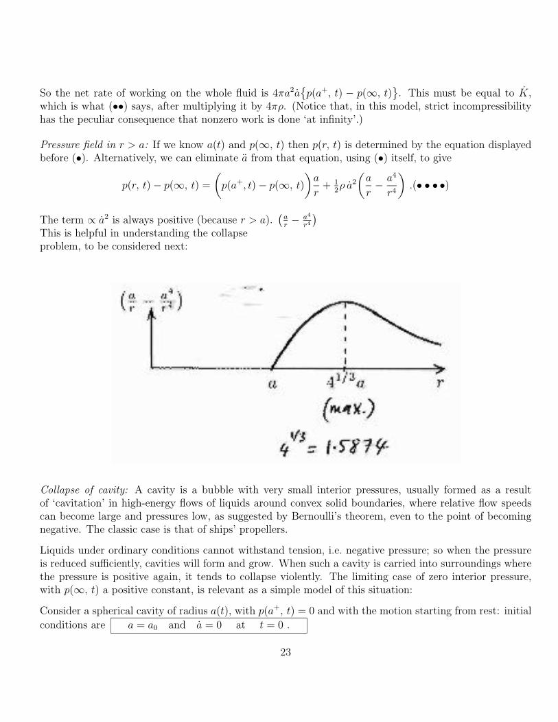
that the singularity at a = 0 is integrable giving a finite time interval t− tc, and that t− tc ∝ a5/2 hencea ∝ (t− tc)2/5.) More precisely, and confirming the finiteness of tc ,

tc =

∫ a0

0

da[2

3

p∞ρ

(a3

0

a3− 1

)]1/2=

(3ρa2

0

2p∞

)1/2 ∫ 1

0

dα

{(1/α)3 − 1}1/2(α = a/a0)

= 0.92

(ρa2

0

p∞

)1/2

,

from numerical integration.

24

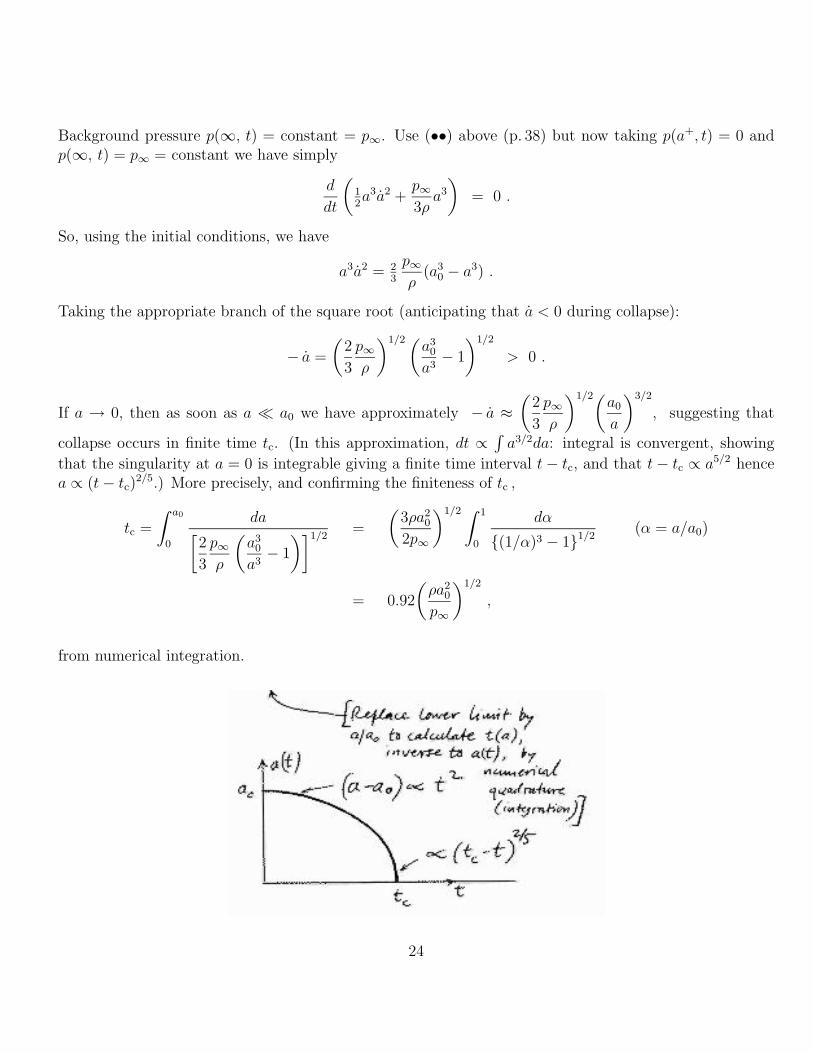
The expression (• • • •) for p(r, t) tell us something interesting about the way the pressure p(r) varieswithin the liquid; (• • • •) simplifies to

p(r, t) = p∞

(1− a

r

)+ 1

2ρ a2

(a

r− a4

r4

).

(Remember that p(a+, t) = 0 now.) As remarked before, the term ∝ a2 is always positive (because r > a);see graph above (and note maximum value is at r/a = 41/3 = 1.5874). Since a increases without bound,an interior pressure maximum must form:

This contrasts with the earliest stages of collapse, with (a0 − a) ∝ t2 and a ∝ t, for t � tc. (Seesketch graph of a(t) at bottom of previous page, and check the behaviour (a − a0) ∝ t2 by consider-

ing∫ 1

1−ε {(1/α)3 − 1}−1/2dα, where ε � 1.) Then the first term in the expression p∞

(1− a

r

)+

12ρ a2

(a

r− a4

r4

)dominates the second; there is no pressure maximum, implying that ∇p is directed

radially outward everywhere. Hence particle accelerations Du/Dt are radially inward everywhere, at thisearly stage.

In the latest stages, after formation of the pressure maximum, with a → 0 like (t − tc)2/5, and a2 → ∞,the second term, the term ∝ a2, dominates the first. The pressure maximum has formed and is movinginward, and, in the limit a → 0, its value asymptotically approaches the value given by the second termalone, at r ≈ 41/3a. That value can be seen, from

substituting a ≈(

2

3

p∞ρ

)1/2(a0

a

)3/2

, to be asymptoticallyp∞44/3

a30

a3.

25

E.g. ata

a0

=1

10, find p∞ = 1 atm ⇒ pmax ∼ 160 atm

and a ∼ 260 ms−1

(approaching pressures that can melt some metals!)

(Remember 1 atm = 105Pa = 105N m−2; common liquids, e.g. water, have ρ ≈ 103kg m−3; so p∞/ρ ≈102m s−2.)

Again, ata

a0

=1

100, find p∞ = 1 atm ⇒ pmax ∼ 160 000 atm

and a ∼ 8 000 ms−1

(But now the theory has well and truly predicted its own breakdown: 8 000 ms−1 is well over the soundspeed in most liquids, e.g. for water, sound speed ∼ 1500 m s−1, and incompressibility won’t be a goodapproximation.)

The pressure maximum forms because, in our incompressible model, the inward flow at any fixed positionr > 0 outside the cavity decelerates, toward zero velocity, as the cavity volume becomes vanishingly small(a� r). (You should check that |u| → 0 at fixed r; recall, e.g., that φ = −a2a/r.) Inward deceleration oroutward acceleration corresponds to inward-directed ∇p.

*When departures from spherical symmetry are allowed for, it turns out that the extreme velocities and pressures tend,unfortunately, to be directed toward the nearest solid surface in the form of tiny but powerful jets within the bubble at itsfinal stage of collapse. This can cause what is called ‘cavitation damage’.*

§3.5 Translating sphere, and inertial reaction to acceleration

First consider steady motion:

Recall the velocity potential for uniform flow past fixed sphere (§3.2):

φ = U cos θ

(r +

a3

2r2

)26

Velocity in spherical polars: u = ∇φ =

[U cos θ

(1− a3

r3

), − U sin θ

(1 +

a3

2r3

), 0

].

Calculate pressure force on sphere, using time-dependent Bernoulli:

∂φ

∂t+ 1

2|u|2 +

p

ρ+ Φ = H(t) = p∞ + 1

2U2

(steady) (no body forces)

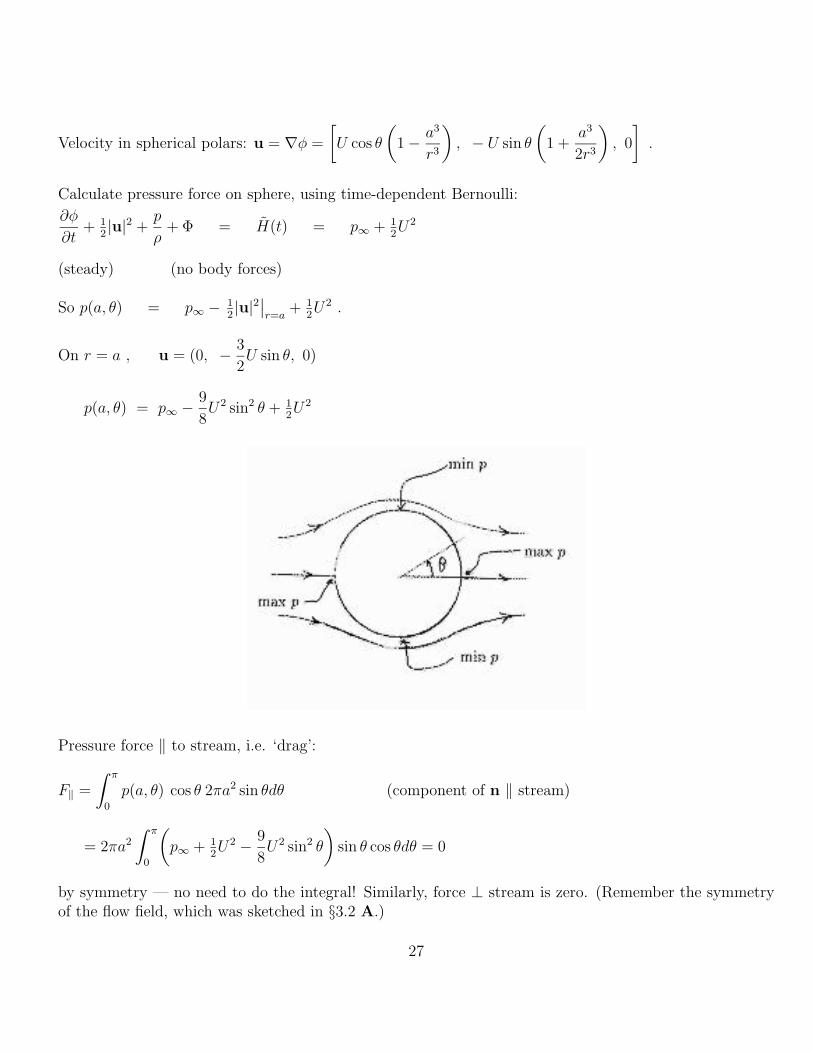
So p(a, θ) = p∞ − 12|u|2∣∣r=a

+ 12U2 .

On r = a , u = (0, − 3

2U sin θ, 0)

p(a, θ) = p∞ −9

8U2 sin2 θ + 1

2U2

Pressure force ‖ to stream, i.e. ‘drag’:

F‖ =

∫ π

0

p(a, θ) cos θ 2πa2 sin θdθ (component of n ‖ stream)

= 2πa2

∫ π

0

(p∞ + 1

2U2 − 9

8U2 sin2 θ

)sin θ cos θdθ = 0

by symmetry — no need to do the integral! Similarly, force ⊥ stream is zero. (Remember the symmetryof the flow field, which was sketched in §3.2 A.)

27

Pressure has two maxima (at the front and rear stagnation points), and a minimum on the bisecting plane⊥ stream.

Energy considerations (§3.7 below) are enough to show that the drag, or component of net force parallel tothe stream, must vanish for potential flow round any 3-D body (§3.7 below). This is called d’Alembert’sparadox — ‘paradox’ because experience is that 3-D bodies moving steadily in real fluids do experiencenonzero drag.

(*It can also be shown, though not from energy considerations, that the ⊥ force vanishes as well — notjust for the sphere, but for any 3-D body in potential flow: Batchelor p. 405.*)

Effects of friction (explanation of the ‘paradox’)

No-force result is correct for inviscid (frictionless) fluids, but often, in real fluids, the effect of frictioncannot be neglected, even when a naive estimate says that it is likely to be small. Potential flow is oftena bad approximation, for flow past solid bodies.

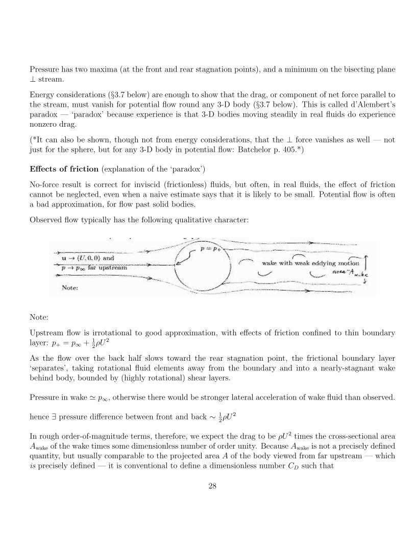
Observed flow typically has the following qualitative character:

Note:

Upstream flow is irrotational to good approximation, with effects of friction confined to thin boundarylayer: p+ = p∞ + 1

2ρU2

As the flow over the back half slows toward the rear stagnation point, the frictional boundary layer‘separates’, taking rotational fluid elements away from the boundary and into a nearly-stagnant wakebehind body, bounded by (highly rotational) shear layers.

Pressure in wake ' p∞, otherwise there would be stronger lateral acceleration of wake fluid than observed.

hence ∃ pressure difference between front and back ∼ 12ρU2

In rough order-of-magnitude terms, therefore, we expect the drag to be ρU2 times the cross-sectional areaAwake of the wake times some dimensionless number of order unity. Because Awake is not a precisely definedquantity, but usually comparable to the projected area A of the body viewed from far upstream — whichis precisely defined — it is conventional to define a dimensionless number CD such that

28

Drag = 12ρU2 A CD .

CD is by convention called the drag coefficient; it is typically a modest fraction of unity, though the precisevalue depends very much on circumstances (e.g. on just how small the viscosity is, and whether the bodysurface is rough or smooth). As the rough argument just given suggests, CD is numerically close to unityif the wake is ‘fat’ in the sense that A ∼ Awake.

*It is the cross-sectional area of the wake that is sensitive to circumstance. With a thin wake, conditionsare closer to ideal potential-flow conditions, and CD can be a fairly small fraction of unity. This can occurfor a solid sphere in certain (complicated) circumstances (to do with very delicate properties of turbulentboundary layers).*

Summary so far: Potential flow is a bad model for steady flow past solid bodies like spheres, indeed anysuch body that is not highly streamlined, like an aircraft. Potential flow is a good model for:

•Flow past or around bubbles•Acceleration of rigid bodies, for short time intervals such that there is

insufficient time for vorticity to escape from boundaries•Small amplitude oscillations.

§3.6 Accelerating sphere

We continue to neglect gravity, and solve in a frame such that fluid is at rest at∞ (otherwise it is necessaryto take account of non-inertial effects, i.e. ‘fictitious forces’ in a non-inertial reference frame). Consider asphere of radius a, centre x0(t), with dx0/dt = U(t). Write r = |x−x0|. Outward normal n = (x−x0)/r .Potential problem to solve is

∇2 φ = 0

∇ φ→ 0 as r →∞n .∇φ = n.U(t) on r = a .

Rather than solving from scratch, we can use the solution constructed previously, on p. 27, with cos θ =n.U/|U| , after subtracting the uniform flow at infinity. (The superposition principle for the linear equation∇2φ = 0 says that we still have a potential flow. But the sphere is now moving in the −z direction; toreverse this we replace U on p. 27 by −|U| here.) The result is

φ = − |U|a3

2r2cos θ = − U.(x− x0)a3

2|x− x0|3.

29

Rewriting the solution in vector notation frees us from any particular coordinate system.(Exercise: check that this does solve the above boundary-value problem!)

Note that there is no memory in the problem — the solution at any instant depends only on boundary conditions at thatinstant. So solving for φ is indifferent to whether or not U and x0 are functions of t.

Taking ∂/∂t, we have

∂φ

∂t= − U.(x− x0)a3

2|x− x0|3+ U.∇

{U.(x− x0)a3

2|x− x0|3

}= U.∇φ = U.u

(The second term comes from the time-dependence of x0, using the chain rule, along with the fact that the gradient withrespect to x0 is minus the gradient with respect to x, of any function of x− x0 alone.)

Now use time-dependent Bernoulli, H = H∞,

p = p∞ − ρ∂φ

∂t− 1

2ρ|u|2 = p∞ + ρU.

(x− x0)a3

2|x− x0|3− 1

2ρ|u|2 − ρU.u .

Force F on sphere (now taking x0 = 0 w.l.o.g. — no more time differentiation):

F = −∫|x|=a

pn dS = −∫r=a

px

rdS

= −ρ∫r=a

U.x a3

2r3

x

rdS − (p∞ + 1

2ρ|U|2)

∫r=a

n dS + ρ

∫r=a

12|u + U|2n dS

In components, Fi = −M∗ijUj where

M∗ij = ρ

∫r=a

a3xj2a3

xiadS = 1

2ρ

∫r=a

xixjadS = 1

2ρ 4πa3 1

3δij .

(Easiest proof of last step: note that the integral must be an isotropic tensor, hence ∝ δij, so it is enoughto evaluate the trace of the integral, i.e., to set i = j and sum, noting that xixi = a2 and noting also thatδjj = 3.) So:

M∗ij =

2πρa3

3δij = 1

2ρV δij = M∗δij , say; so F = −1

2ρV U.

So for the sphere, F = −M∗U = −12ρV U. It is natural to call M∗ = 2

3πρ a3 = 1

2ρV the

added mass, or virtual mass, for a sphere.

30

(*For a general, non-isotropic, body the added mass becomes a general, non-isotropic tensor quantity, M∗ij , not ∝ δij , becausethe integral involving xixj will emphasize some directions more than others.*)

As the sphere is accelerated, a body of fluid is accelerated with it. Because the fluid exerts a force on thesphere, the sphere must exert a force on the fluid, in the opposite direction (Newton’s third law) — it isof course given by the same calculation as above, with the sign of n reversed.

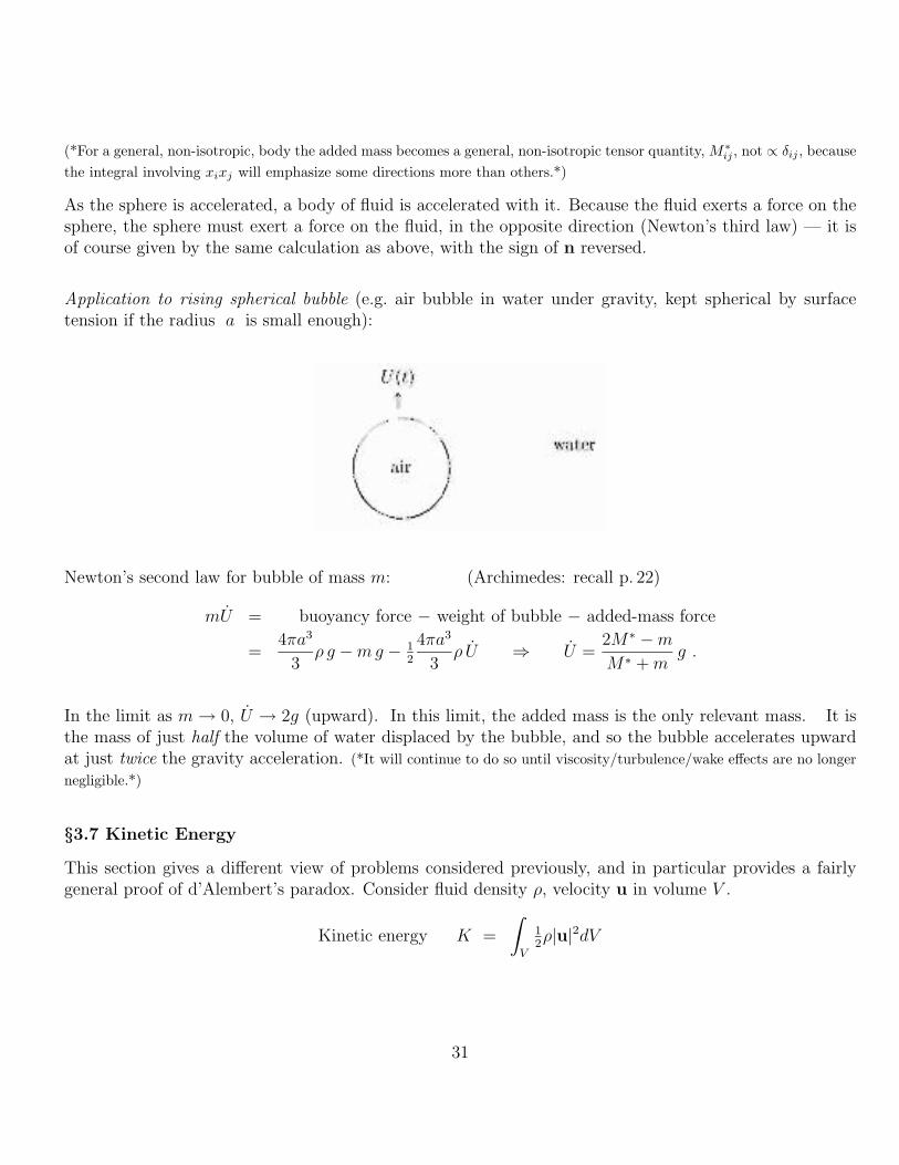
Application to rising spherical bubble (e.g. air bubble in water under gravity, kept spherical by surfacetension if the radius a is small enough):

Newton’s second law for bubble of mass m: (Archimedes: recall p. 22)

mU = buoyancy force − weight of bubble − added-mass force

=4πa3

3ρ g −mg − 1

2

4πa3

3ρ U ⇒ U =

2M∗ −mM∗ +m

g .

In the limit as m→ 0, U → 2g (upward). In this limit, the added mass is the only relevant mass. It isthe mass of just half the volume of water displaced by the bubble, and so the bubble accelerates upwardat just twice the gravity acceleration. (*It will continue to do so until viscosity/turbulence/wake effects are no longernegligible.*)

§3.7 Kinetic Energy

This section gives a different view of problems considered previously, and in particular provides a fairlygeneral proof of d’Alembert’s paradox. Consider fluid density ρ, velocity u in volume V .

Kinetic energy K =

∫V

12ρ|u|2dV

31

Assuming potential flow, with u = ∇φ, we have

K = 12ρ

∫V

(∇φ)2 dV = 12ρ

∫V

(∇.(φ∇φ)− φ∇2φ

)dV = 1

2ρ

∫S

n.(φ∇φ) dS

= 12ρ

∫S

φu.n dS

where S is the surface bounding V , and n is now the unit normal vector pointing outward from the fluid.

If the velocity of points on the boundary is denoted by Uboundary then, by the kinematic boundary condition,Uboundary.n = u.n = n.∇φ on S and hence

K = 12ρ

∫φUboundary.n dS.

(You should check that this agrees with what was calculated in the special case of p. 38.)

Now apply this to our standard case of the translating sphere in a fluid at rest far from sphere. Take theorigin to be instantaneously coincident with the centre of the sphere, x0 = 0, and take the volume V ofintegration to be the volume a < |x| < R, where R� a. Then, by above,

K = 12ρ

∫|x|=R

φu.er dS − 12ρ

∫|x|=a

φU.er dS,

where er is the unit vector in the radial direction.

The first integral → 0 as R → ∞. For we have φ = −Ua3 cos θ/(2r2), so on |x| = R, φ ∼ R−2, andu.er ∼ R−3, and since dS ∼ R2 the first integral ∼ R−3,→ 0 as R→∞.

Hence

K = −12ρ

∫ π

θ=0

− Ua3 cos θ

2a2U cos θ 2πa2 sin θ dθ (−

∫ π0

cos2 θ d(cos θ) = 23)

= 12ρU2 2πa3

3= 1

2(1

2ρV )U2 = 1

2M∗ U2

So the effective mass M∗ of fluid moving with the sphere, and giving rise to kinetic energy (K.E.) of thefluid, is the same as that accelerating with the sphere, and giving rise to the force on it.

This must be the case; we are merely checking that the whole picture is self-consistent. If the sphereaccelerates, then

rate of change of K.E. = rate of working of sphere on fluid

i.e., M∗U.U = − F.U .

32

(There is no pressure-working at ∞ because u.er ∼ R−3, cf. R−2 on p. 38.)

So F = −M∗U + F⊥ where F⊥ is a possible force perpendicular to the direction of motion.

Note that the energy argument cannot tell us anything about F⊥, because F⊥ does no work.

*But the energy argument, applied to a body of arbitrary fixed shape, does, now, lead to a general proof of d’Alembert’sparadox if we are prepared to assume — this can be proven, but there is no room here! — that the first integral, the integralover |x| = R in the above expression for K, still vanishes as R→∞ even if the body is no longer a sphere.

(The proof takes the general separation-of-variables solution for φ, and shows that all the terms O(r−1) vanish because massis conserved and the body has constant volume, so that in the far field we have the same magnitude as above, O(R−3),for the integral over |x| = R, plus smaller terms O(R−4), O(R−5,),... Batchelor’s book covers this point thoroughly. Theargument is like that to be given on p. 49: the body has fixed volume and so there are no r−1 terms in the general solutionon p. 25 and its 3-D generalization. Nor, of course, are there any positive powers of r.)*

The energy argument now says that (for a body of arbitrary shape) Fi = −M∗ijUj +F⊥ j, and so the drag,

F− F⊥, must vanish when U = 0.

(*F⊥ can also be shown to be zero for a three-dimensional body of any shape — essentially by applying the momentumintegral over the same volume V , but integrands evanesce more slowly and the argument about R → ∞ is more delicate!Notice the implication: a glider or other fixed-wing aircraft could not stay airborne if the flow past it were everywhere apotential flow. Yet efficient aircraft, especially high performance gliders, are designed so that the flow past them is as closeto potential/irrotational as can be managed. Fixed-wing aircraft and gliding birds stay up because, occupying a relativelysmall volume, there is a pair of trailing vortices coming off the wings; and |∇×u| is anything but small at the centre of anysuch vortex. Trailing vortices, in other words, are not incidental features; they are indispensable to staying up! (See p. 50.)*)

§3.8 Steady flow past cylinder with circulation: 2-D lift forces

Two-dimensional flow is conceptually important because for the first time we get a simple potential-flowmodel in which there is a lift force, that is, a nonzero force component F⊥ at right angles to the streamU. This was already implied by the crowding of streamlines, solutions on p. 29.

We revert to considering steady flow only; it is again convenient to use the frame in which the obstacle —an infinitely long cylinder — is stationary and the flow velocity at infinity is U.

Now recall the solution for potential flow round the cylinder with circulation κ (last item in §3.2B), p. 29:

φ = U cos θ

(r +

a2

r

)+κθ

2π

(U = |U|

)u = ∇φ =

(U cos θ

(1− a2

r2

), − U sin θ

(1 +

a2

r2

)+

κ

2πr

)(components in 2-D polars)

33

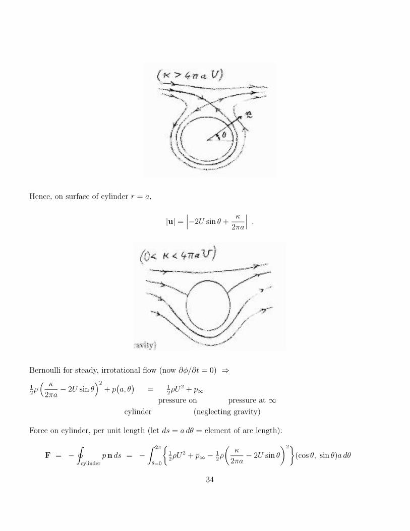
Hence, on surface of cylinder r = a,

|u| =∣∣∣−2U sin θ +

κ

2πa

∣∣∣ .

Bernoulli for steady, irrotational flow (now ∂φ/∂t = 0) ⇒

12ρ( κ

2πa− 2U sin θ

)2

+ p(a, θ)

= 12ρU2 + p∞

pressure on pressure at ∞cylinder (neglecting gravity)

Force on cylinder, per unit length (let ds = a dθ = element of arc length):

F = −∮

cylinder

pn ds = −∫ 2π

θ=0

{12ρU2 + p∞ − 1

2ρ

(κ

2πa− 2U sin θ

)2}(cos θ, sin θ)a dθ

34

= 12ρa

∫ 2π

0

(AU2 sin2 θ − 2κU sin θ

πa

)(cos θ, sin θ) dθ where A is a constant,

about whose value we don’t care because its contribution to the integral is zero, by inspection: note thatsin2 θ cos θ, sin3 θ and sin θ cos θ all integrate to zero, being odd functions about some point in (0, 2π).

Recall too that∫ 2π

0sin2 θ dθ = π.

=−ρκUπ

∫ 2π

θ=0

(0, sin2 θ)dθ

= (0, −ρκU) per unit length .

So there is a lift force F⊥ perpendicular to the oncoming flow, of magnitude |F⊥| = |ρκU |.

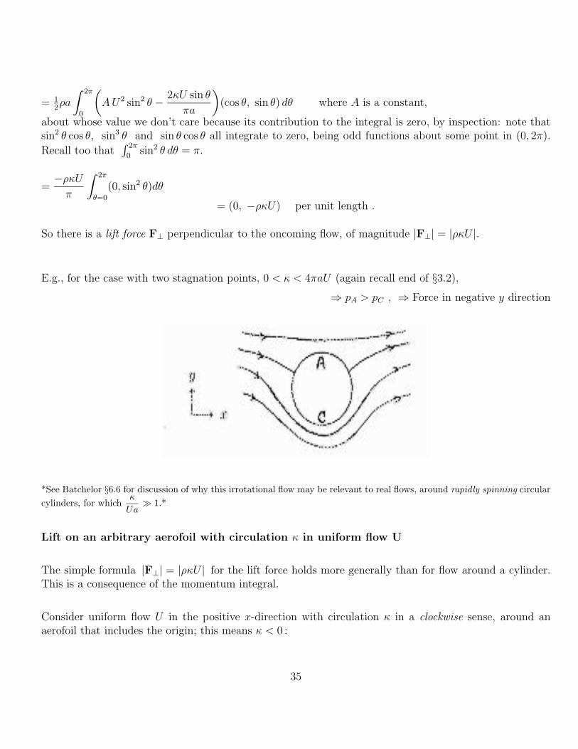
E.g., for the case with two stagnation points, 0 < κ < 4πaU (again recall end of §3.2),

⇒ pA > pC , ⇒ Force in negative y direction

*See Batchelor §6.6 for discussion of why this irrotational flow may be relevant to real flows, around rapidly spinning circularcylinders, for which

κ

Ua� 1.*

Lift on an arbitrary aerofoil with circulation κ in uniform flow U

The simple formula |F⊥| = |ρκU | for the lift force holds more generally than for flow around a cylinder.This is a consequence of the momentum integral.

Consider uniform flow U in the positive x-direction with circulation κ in a clockwise sense, around anaerofoil that includes the origin; this means κ < 0 :

35

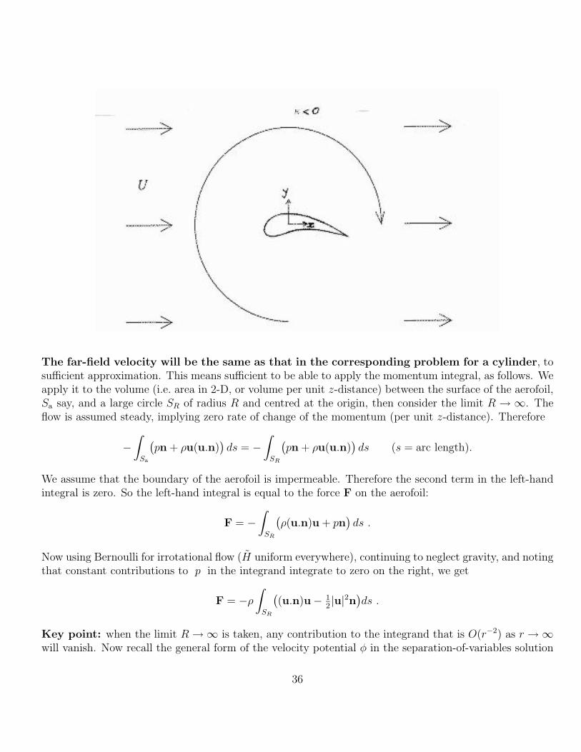
The far-field velocity will be the same as that in the corresponding problem for a cylinder, tosufficient approximation. This means sufficient to be able to apply the momentum integral, as follows. Weapply it to the volume (i.e. area in 2-D, or volume per unit z-distance) between the surface of the aerofoil,Sa say, and a large circle SR of radius R and centred at the origin, then consider the limit R → ∞. Theflow is assumed steady, implying zero rate of change of the momentum (per unit z-distance). Therefore

−∫Sa

(pn + ρu(u.n)

)ds = −

∫SR

(pn + ρu(u.n)

)ds (s = arc length).

We assume that the boundary of the aerofoil is impermeable. Therefore the second term in the left-handintegral is zero. So the left-hand integral is equal to the force F on the aerofoil:

F = −∫SR

(ρ(u.n)u + pn

)ds .

Now using Bernoulli for irrotational flow (H uniform everywhere), continuing to neglect gravity, and notingthat constant contributions to p in the integrand integrate to zero on the right, we get

F = −ρ∫SR

((u.n)u− 1

2|u|2n

)ds .

Key point: when the limit R→∞ is taken, any contribution to the integrand that is O(r−2) as r →∞will vanish. Now recall the general form of the velocity potential φ in the separation-of-variables solution

36

for Laplace’s equation in 2-D polars (p. 27). We may ignore all the terms in rn for n > 2 because they allgive unbounded velocities u = ∇φ at large distances from the origin. We may also ignore the log r term,because if that term were nonzero then there would be a finite mass flux to or from infinity, hence intoor out of the aerofoil, by mass conservation (contradicting impermeability). Therefore, in the notation ofp. 27, with α1 = 0 and A1 = U to match the uniform flow at infinity, and B0 = κ/2π as on p. 28:

φ = Ur cos θ +κ

2πθ +

∞∑n=1

{Bnr

−n cos(nθ + βn)}.

Taking the gradient and noting that the resulting contribution from∑∞

n=1 is O(r−2), we have u in polarcomponents:

u =(U cos θ +O(r−2) , − U sin θ +

κ

2πr+O(r−2)

)(as r →∞).

Substituting this far-field expression into u.n and 12|u|2 and noting that n = er and hence u.n = u.er =

U cos θ +O(R−2), we see that the Cartesian components of F are

F = −ρ∫ 2π

0

(U cos θ +O(R−2)

)(U − κ sin θ

2πR+O(R−2),

κ cos θ

2πR+O(R−2)

)Rdθ

+ρ

∫ 2π

0

12

(U2 − κU sin θ

πR+O(R−2)

)(cos θ, sin θ)Rdθ

(because n = er = (cos θ, sin θ)). Evaluating the integrals in the limit R → ∞, and again using∫cos θ dθ =

∫sin θ cos θ dθ = 0, and

∫cos2 θ dθ =

∫sin2 θ dθ = π, gives (in Cartesian components)

F = (0, − ρκU) .

*Generation of circulation (to give the lift ρκU)

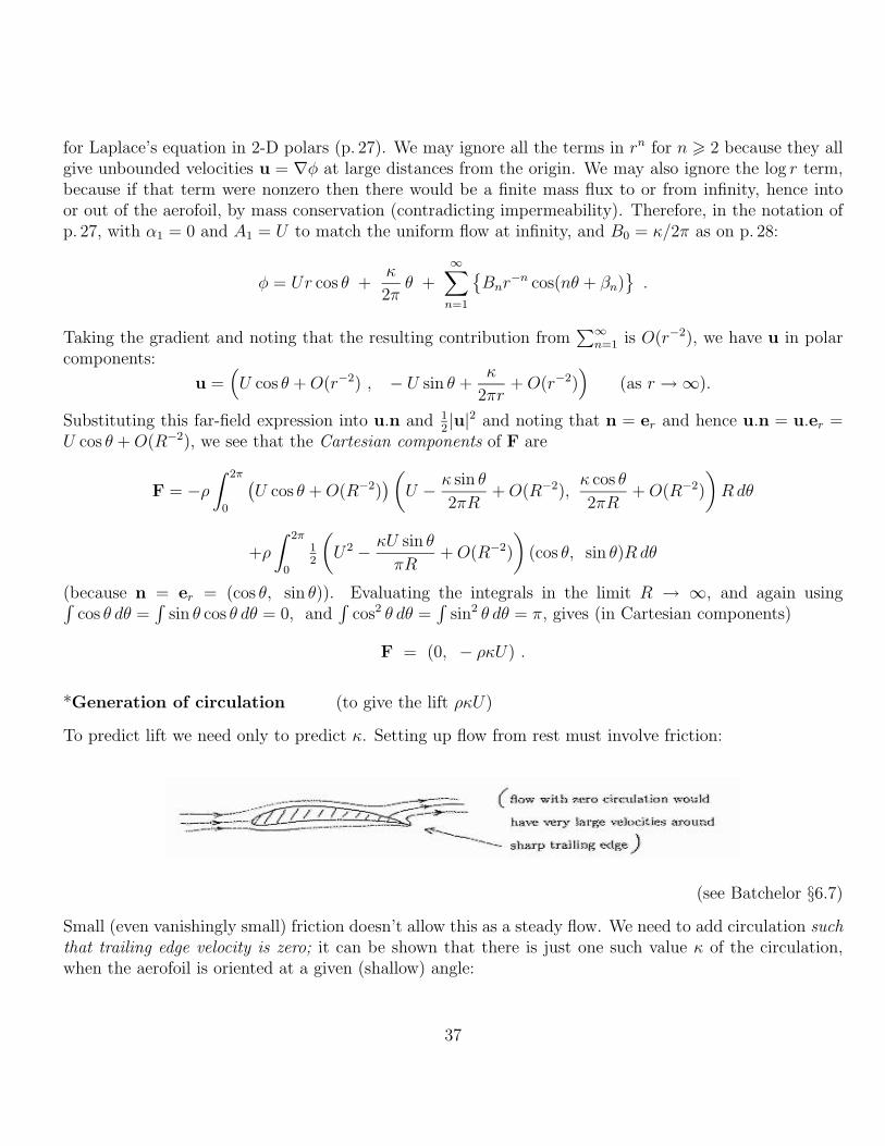
To predict lift we need only to predict κ. Setting up flow from rest must involve friction:

(see Batchelor §6.7)

Small (even vanishingly small) friction doesn’t allow this as a steady flow. We need to add circulation suchthat trailing edge velocity is zero; it can be shown that there is just one such value κ of the circulation,when the aerofoil is oriented at a given (shallow) angle:

37

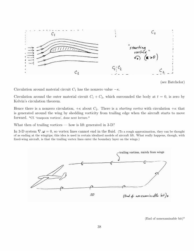
(see Batchelor)

Circulation around material circuit C1 has the nonzero value −κ.

Circulation around the outer material circuit C1 + C2, which surrounded the body at t = 0, is zero byKelvin’s circulation theorem.

Hence there is a nonzero circulation, +κ about C2. There is a starting vortex with circulation +κ thatis generated around the wing by shedding vorticity from trailing edge when the aircraft starts to moveforward. *Cf. ‘teaspoon vortices’, done next lecture.*

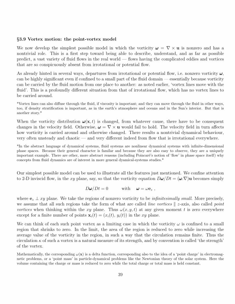
What then of trailing vortices — how is lift generated in 3-D?

In 3-D system ∇. ωωω = 0, so vortex lines cannot end in the fluid. (To a rough approximation, they can be thoughtof as ending at the wingtips; this idea is used in certain idealized models of aircraft lift. What really happens, though, withfixed-wing aircraft, is that the trailing vortex lines enter the boundary layer on the wings.)

(End of nonexaminable bit)*

38

§3.9 Vortex motion: the point-vortex model

We now develop the simplest possible model in which the vorticity ωωω = ∇ × u is nonzero and has anontrivial role. This is a first step toward being able to describe, understand, and as far as possiblepredict, a vast variety of fluid flows in the real world — flows having the complicated eddies and vorticesthat are so conspicuously absent from irrotational or potential flow.

As already hinted in several ways, departures from irrotational or potential flow, i.e. nonzero vorticity ωωω,can be highly significant even if confined to a small part of the fluid domain — essentially because vorticitycan be carried by the fluid motion from one place to another: as noted earlier, ‘vortex lines move with thefluid’. This is a profoundly different situation from that of irrotational flow, which has no vortex lines tobe carried around.

*Vortex lines can also diffuse through the fluid, if viscosity is important; and they can move through the fluid in other ways,too, if density stratification is important, as in the earth’s atmosphere and oceans and in the Sun’s interior. But that isanother story.*

When the vorticity distribution ωωω(x, t) is changed, from whatever cause, there have to be consequentchanges in the velocity field. Otherwise, ωωω = ∇× u would fail to hold. The velocity field in turn affectshow vorticity is carried around and otherwise changed. There results a nontrivial dynamical behaviour,very often unsteady and chaotic — and very different indeed from flow that is irrotational everywhere.

*In the abstract language of dynamical systems, fluid systems are nonlinear dynamical systems with infinite-dimensionalphase spaces. Because their general character is familar and because they are also easy to observe, they are a uniquelyimportant example. There are other, more abstract reasons (including Poincare’s notion of ‘flow’ in phase space itself) whyconcepts from fluid dynamics are of interest in more general dyamical-systems studies.*

Our simplest possible model can be used to illustrate all the features just mentioned. We confine attentionto 2-D inviscid flow, in the xy plane, say, so that the vorticity equation Dωωω/Dt = (ωωω.∇)u becomes simply

Dωωω/Dt = 0 with ωωω = ωez ,

where ez ⊥ xy plane. We take the regions of nonzero vorticity to be infinitesimally small. More precisely,we assume that all such regions take the form of what are called line vortices ‖ z-axis, also called pointvortices when thinking within the xy plane. Thus ω(x, y, t) at any given moment t is zero everywhereexcept for a finite number of points xi(t) = (xi(t), yi(t)) in the xy plane.

We can think of each such point vortex as a limiting case in which the vorticity ω is confined to a smallregion that shrinks to zero. In the limit, the area of the region is reduced to zero while increasing theaverage value of the vorticity in the region, in such a way that the circulation remains finite. Thus thecirculation κ of such a vortex is a natural measure of its strength, and by convention is called ‘the strength’of the vortex.

Mathematically, the corresponding ω(x) is a delta function, corresponding also to the idea of a ‘point charge’ in electromag-netic problems, or a ‘point mass’ in particle-dynamical problems like the Newtonian theory of the solar system. Here thevolume containing the charge or mass is reduced to zero while the total charge or total mass is held constant.

39

Recall from §3.2a the velocity potential for a point vortex at the origin, with circulation κ, i.e. with‘strength’ κ (and going back to standard sign convention):

φ = κθ/2π,

and recall that this satisfies Laplace’s equation everywhere except at the origin. The corresponding velocityfield is

u = ∇φ =κ

2πreθ =

κ

2π

ez × x

|x|2=

κ

2π(− y

x2 + y2,

x

x2 + y2)

where the components in the last expression are referred to Cartesian axes.

Laplace’s equation is linear, so we can linearly superpose a finite number N of point vortices with differentstrengths and positions xi (i = 1, ...N), thus

φ(x) =N∑i=1

κiθi2π

and u(x) =N∑i=1

κi2π

ez × (x− xi)

|x− xi|2(x 6= xi ∀i).(∗)

This, by linearity, satisfies Laplace’s equation everywhere except at x = xi. The crucial point now is thatwe satisfy Dωωω/Dt = 0 by requiring that the x = xi are functions of time t such that:

Each vortex is moved by the velocity field due to all the other vortices.(∗∗)

This is consistent! The velocity field of one vortex by itself cannot move that vortex. An isolated vortexjust sits in one place, spinning but doing nothing else (as is obvious by symmetry; no particular directionis distinguished). The dynamical system thus defined consists of a set of N first-order nonlinear ordinarydifferential equations for the N functions xi(t):

xi(t) =∑j 6=i

κj2π

ez × (xi − xj)

|xi − xj|2(i = 1, ...N) , (∗∗∗)

where xi means the time derivative, as usual, dxi(t)/dt, and the summation is from j = 1 to N butomitting the term for which j = i.

*Being nonlinear, these differential equations must usually be solved numerically, which is easy these days on any personalcomputer for modest values of N . It is known that when N > 4 the system behaves chaotically, in most cases, implying anexponential blowup in sensitivity to initial conditions as time increases. Such sensitivity is liable to be important wheneverthe equations are integrated over timescales much longer than tvort ∼ 2πL2/κ, if κ is a typical vortex strength and L atypical separation between vortices so that |xi| has typical values of order 2πκ/L. This is fundamentally like the initial-condition sensitivity that limits the timespan of weather forecasting. It can be shown that cyclones and anticyclones in thereal atmosphere behave in some respects like the vortices in our 2-D point-vortex model, with tvort values of the order of aday or two. (The real behaviour is closer to 2-D than 3-D because of the stable density stratification, but that is anotherstory.) The expectation of chaotic behaviour for N > 4 correctly suggests why it is impracticable to forecast the weather indetail many days ahead.*

40

There are a few simple cases of (∗∗∗) that are both soluble analytically and practically important.

The simplest is what is called a vortex pair, the case N = 2 and κ1 = −κ2 = κ, say. By inspection of(∗∗∗) we see that x2(t) = x1(t),= U say, from which it follows at once that d(x1 − x2)/dt = 0, so that(x1 − x2) is a constant of the motion. The line segment joining the two vortices is constant in length andorientation.

Because of the vector products in (∗∗∗), we see also that U ⊥ (x1 − x2). The two vortices move as one,with the same constant velocity U having magnitude

|U| = |κ|2π|x1 − x2|

and directed at right angles to the line joining the two vortices.

*This property is the 2-D counterpart of the way a circular vortex ring in 3-D, sometimes made visible as a smoke ring,translates through a fluid in the direction at right angles to its plane. The vortex-pair solution also adds to our understandingof how aircraft stay up: the trailing vortices extend a long way behind the aircraft and behave very like our simple 2-Dvortex pair, with U directed downward. One can show that the associated velocity field, (∗) with N = 2, carries nearby airpredominantly downward as well, as might be expected from Newton’s third law. To stay up, the aircraft has to push airdown.*

Use of ‘images’

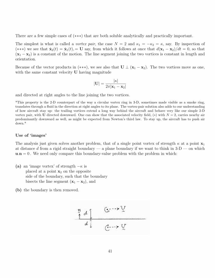
The analysis just given solves another problem, that of a single point vortex of strength κ at a point x1

at distance d from a rigid straight boundary — a plane boundary if we want to think in 3-D — on whichu.n = 0 . We need only compare this boundary-value problem with the problem in which:

(a) an ‘image vortex’ of strength −κ isplaced at a point x2 on the oppositeside of the boundary, such that the boundarybisects the line segment (x1 − x2), and

(b) the boundary is then removed.

41

This last problem is the same problem as that just solved, the vortex-pair problem; so we already knowthe solution. The points x1 and x2 move with the constant velocity x1 = x2 = U parallel to the formerboundary, with |U| = |κ|/4πd. Moreover, by symmetry, u.n = 0 where the boundary was located; so wecan put the boundary back without changing anything!

More specifically, and taking the boundary to be y = 0 — the yz plane if we want to think in 3-D — wehave solved the following boundary value problem. We have satisfied Laplace’s equation ∇2φ = 0 in y > 0with boundary conditions of evanescence at infinity together with

∂φ

∂y= 0 on y = 0 i.e., u.n = 0 with n = (0, 1)

and

φ(x)→ κθ1

2πas |x− x1| → 0 ,

where θ1 is the angle giving the direction of (x−x1), that is, θ1 = arctan {(y − y1)/(x− x1)}. Defining also(x2, y2) = (x1, −y1), the image point, and θ2 = arctan {(y − y2)/(x− x2)} = arctan {(y + y1)/(x− x1)},we see that the velocity potential and the corresponding velocity field are, for all x 6= x1, x2,

φ(x) =κθ1

2π− κθ2

2π⇒ u(x) =

κez2π×{

(x− x1)

|x− x1|2− (x− x2)

|x− x2|2

}.

2-vortex problems in general

The properties that x1(t) ⊥ (x1 − x2) and x2(t) ⊥ (x1 − x2) can be seen, again by inspection of (∗∗∗), tohold for all point-vortex problems with N = 2, including, that is, cases where κ1 6= κ2. All these 2-vortexproblems share the property that |x1−x2| is a constant of the motion, making them all analytically soluble.The motion is always on arcs of circles, if we include straight lines by regarding them as circles of infiniteradius.

In the case κ1 = κ2 = κ, for instance, the two vortices move around each other at speed |U| = |κ|/4πa inthe same circle, of radius a say, centred on the midpoint xmid = 1

2(x1 + x2). The midpoint is, indeed,

stationary: x1 = −x2, so that xmid = 0. For further variations on this theme, try Q1 on Ex. Sheet 3.)

More complicated boundaries:

The method of images can handle more elaborate boundary configurations. The next simplest is twoboundaries forming a right-angled corner, say the positive x and y axes. With this configuration, a singlepoint vortex of strength κ at (x1 > 0, y1 > 0) has three images, at (x1, − y1), (−x1, y1), (−x1, − y1)with strengths respectively −κ, −κ, κ. From (∗∗∗) we have

x1 =κ

2π

{1

2y1

− y1

2(x21 + y2

1)

}=

κ

4π

x21

y1(x21 + y2

1)

42

and

y1 =κ

2π

{− 1

2x1

+x1

2(x21 + y2

1)

}= − κ

4π

y21

x1(x21 + y2

1).

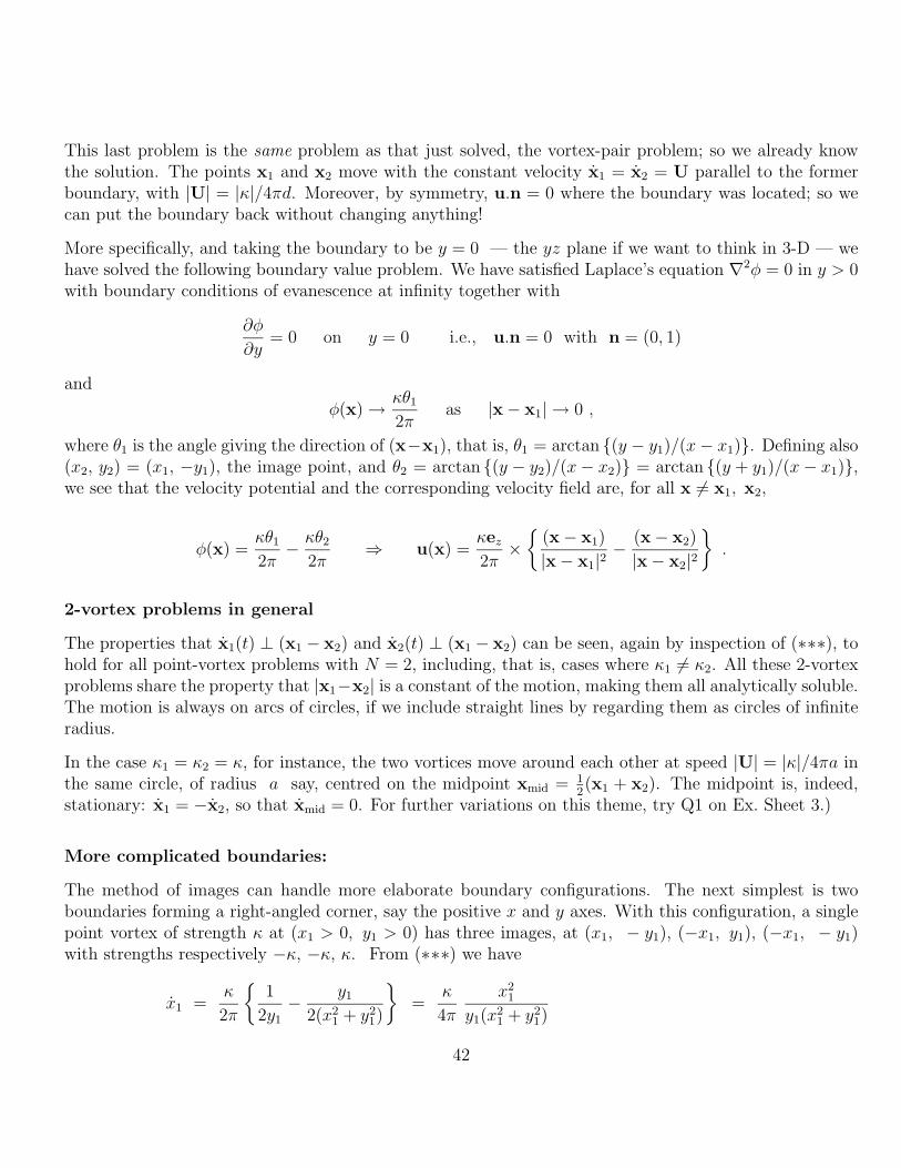
It is easy to deduce the path of the vortex, because

dy1

dx1

=y1

x1

= −(y1

x1

)3

,

which can be integrated to give1

x21

+1

y21

= constant .

The path is sketched below.

By removing one boundary, we see that the same solution describes a vortex pair approaching a singleboundary. The two vortices move apart.

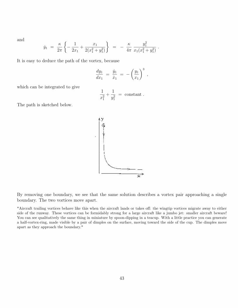
*Aircraft trailing vortices behave like this when the aircraft lands or takes off: the wingtip vortices migrate away to eitherside of the runway. These vortices can be formidably strong for a large aircraft like a jumbo jet: smaller aircraft beware!You can see qualitatively the same thing in miniature by spoon-dipping in a teacup. With a little practice you can generatea half-vortex-ring, made visible by a pair of dimples on the surface, moving toward the side of the cup. The dimples moveapart as they approach the boundary.*

43

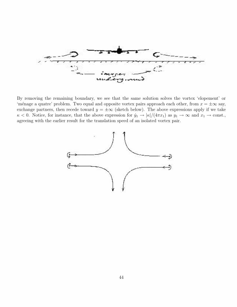
By removing the remaining boundary, we see that the same solution solves the vortex ‘elopement’ or‘menage a quatre’ problem. Two equal and opposite vortex pairs approach each other, from x = ±∞ say,exchange partners, then recede toward y = ±∞ (sketch below). The above expressions apply if we takeκ < 0. Notice, for instance, that the above expression for y1 → |κ|/(4πx1) as y1 → ∞ and x1 → const.,agreeing with the earlier result for the translation speed of an isolated vortex pair.

44