arX

iv:1

710.

0005

9v1

[co

nd-m

at.s

tat-

mec

h] 1

8 Se

p 20

17

Finite-Range Coulomb Gas Models of Banded Random Matrices and Quantum

Kicked Rotors

Akhilesh Pandey,∗ Avanish Kumar,† and Sanjay Puri‡

School of Physical Sciences, Jawaharlal Nehru University, New Delhi-110067, India

(Dated: October 3, 2017)

Dyson demonstrated an equivalence between infinite-range Coulomb gas models and classicalrandom matrix ensembles for study of eigenvalue statistics. We introduce finite-range Coulomb gas(FRCG) models via a Brownian matrix process, and study them analytically and by Monte-Carlosimulations. These models yield new universality classes, and provide a theoretical framework forstudy of banded random matrices (BRM) and quantum kicked rotors (QKR). We demonstrate that,for a BRM of bandwidth b and a QKR of chaos parameter α, the appropriate FRCG model hasthe effective range d = b2/N = α2/N , for large N matrix dimensionality. As d increases, there is atransition from Poisson to classical random matrix statistics.

Introduction.—Random matrices are being used exten-sively in many branches of physics as well as in otherdisciplines. Specifically they have found applications inquantum chaotic systems, such as complex nuclei, atoms,molecules, mesoscopic systems, disordered systems andmodel quantum systems of few degrees of freedom [1–13]. In recent years newer applications have emerged inbiology [14, 15], economics [16, 17] and in communicationengineering [18–20]. In most of these applications, clas-sical ensembles (circular and Gaussian ensembles) haveprovided a basis for understanding statistical propertiesof complex spectra.

Many studies have focused on the crossover from Pois-son to classical random matrix results as a physical pa-rameter is varied. In this context, there have been studiesof diverse systems such as atomic spectra [21], randommatrix models [22], quantum chaotic systems [23–28],Anderson localization [29–31], quark-gluon plasma [32]and neural networks [33]. The crossover has been stud-ied extensively in model systems such as quantum kickedrotors (QKR) and banded random matrices (BRM) [34–45]. There are several routes where by this transition canoccur. In this letter, we provide a theoretical frameworkto obtain spectral properties for such a crossover in QKRand BRM.

Dyson has shown that joint probability distributions(jpd) of the classical ensembles are equilibrium states ofBrownian motion model of N Coulombic particles inter-acting with each other. The positions of the Brownianparticles are identified as the eigenvalues of the randommatrix problem [46]. In his original papers Dyson con-sidered Coulombic particles on a real line with harmonicbinding (referred to as the Gaussian ensembles (GE)) andCoulombic particles on the unit circle (referred to as thecircular ensembles (CE)). In an important generalizationDyson introduced non-harmonic confining potentials onthe real line [47]; see also [27, 48–50]. We will refer to

∗ apandey2006@gmail.com, ap0700@mail.jnu.ac.in† avanishkumar31@gmail.com‡ purijnu@gmail.com

these as linear ensembles. Similar generalizations havebeen done for circular ensembles [51].

In the Dyson model and the extensions above, all par-ticles have pairwise interaction. In this Letter we con-sider natural generalizations to the case where particleshave finite-range interactions. We present analytic andMonte-Carlo results for such ensembles. We refer to theseensembles as finite-range Coulomb gas (FRCG) models.Some of the FRCG analytic results reported here wereobtained earlier by one of the authors [52] and have beenused in [53–55]. The main purpose of this letter is todemonstrate that, for eigenvalue spectra, FRCG modelsare in one-to-one correspondence with BRM and QKR.We will show numerically that the range d of the FRCGmodel equals b2/N = α2/N . Here, b is the bandwidth ofthe BRM, α is the ‘chaos parameter’ of the QKR, andN is the matrix dimensionality. We emphasize that theequality connecting BRM and QKR was discovered em-pirically by Casati, Izrailev and others [36–38, 40]. Fol-lowing Izrailev [36], we expect that the Brownian motionmodel described below for FRCG will have the same cor-respondence for eigenvectors.

FRCG models.—We introduce the jpd of the eigenan-gles for the FRCG models of circular ensembles:

P (θ1, · · · , θN ) = C exp(−βW ). (1)

Here the θj are the eigenangles (in ascending order), C isthe normalization constant, and β is the Dyson param-eter with values 1, 2 and 4. The potential W is givenby

W = −∑

′

log |eiθj − eiθk |+∑

V (eiθj ), (2)

where∑ ′

denotes the sum over all |j − k| ≤ d withj < k. The logarithmic terms represent the finite-rangerepulsive Coulomb gas potential with range d, and V isa one-body (real) periodic potential on the unit circle.Classical ensembles arise for d = N − 1 and V = 0,viz., circular orthogonal ensemble (COE), circular uni-tary ensemble (CUE) and circular symplectic ensemble(CSE) characterized by β = 1, 2, 4 respectively. For thelinear ensembles, we consider eigenvalues xj instead of

2

the eiθj in (1, 2) with V a binding potential on real line.In this case for d = N − 1 and V harmonic, we recoverthe Gaussian orthogonal ensemble (GOE), Gaussian uni-tary ensemble (GUE) and Gaussian symplectic ensemble(GSE) for β = 1, 2, 4 respectively.

Brownian banded matrix process for FRCG.—Theabove jpd can be interpreted as the equilibrium densityof a Brownian process with potential given in (2). This isa natural generalization of the Dyson Brownian motionmodel [46, 47]. We demonstrate this for circular ensem-bles with β = 2 and V = 0. The corresponding Brownianmatrix process involves a stochastic matrix increment viaa BRM of bandwidth d. We introduce a Brownian pro-cess of unitary matrices U(τ):

U(τ + δτ) = U(τ) exp(

i√δτM(τ)

)

. (3)

Here, τ is a fictitious time, δτ is infinitesimal time andthe Brownian increment is given in terms of hermitianrandom matrices M(τ), independent for each τ . M(τ) is

a banded matrix in U(τ)-diagonal representation similar

to the GUE matrix with the constraint that the nonzero

matrix elements of Mjk are only for |j − k| ≤ d. Note

that eigenangles (θ1, · · · , θN ) of U(τ) at each Brownian

step are in ascending order. Thus U(τ) is related to U(0)by a product of infinitesimal random perturbations. For

eigenvector studies one should deal directly with the ma-

trix ensembles {U(τ)}.Using second-order perturbation theory [46, 56] we ob-

tain for the eigenangles θj(τ):

δθj = E(θj)δτ, (δθj)2 = 2β−1δτ. (4)

Here the bar denotes the ensemble average and E(θj)is given by E(θj) = −∂W/∂θj. This defines a Smolu-chowski process with equilibrium density given in (1).The cases with β = 1, 4 can be dealt with similarly re-specting the appropriate symmetries. Later we will makea correspondence between this Brownian motion processand a BRM ensemble with band-width b ≃

√Nd. More-

over we will also demonstrate a direct realization of (3)in QKR with the momentum operator playing the role ofM .

Universality.—We focus on d = O(1), where we expectnew universality classes of fluctuation properties for eachd. To prove this we have used a moment method toobtain the eigenangle density (for large N) as:

ρ̄(θ) ∝ exp [−βV/(βd + 1)] . (5)

Using this we define the unfolded spacings sj = N |θj+1−θj |ρ̄(θj). Thus the jpd, Pd(s1, · · · , sN), of N consecutivespacings is given in the circular case

Pd ∝ δ(

N∑

i=1

si −N)

N∏

j=1

d−1∏

k=0

(sj + · · ·+ sj+k)β . (6)

In the linear case, we again obtain (6), with the constraint∑

sj . N , instead of the δ-function term. For large

N , the difference between the two cases can be ignored.Thus the same fluctuations are obtained for linear andcircular ensembles, and the result is independent of thepotential V . Each d and β gives rise to a unique classof fluctuations. As we will see later, these are realized inQKR and BRM. As d increases, there will be a crossoverfrom Poisson to classical (Wigner-Dyson) statistics.

We will derive analytic results from (6) and supple-ment them with Monte-Carlo (MC) calculations of (1).Our MC approach follows that of [49] for the linear case,and [51] for the circular case. Note that, because of thelogarithmic singularity in (2), the eigenangles (and theeigenvalues in the linear case) do not change their order.

Fluctuation measures.—The statistical quantities of in-terest are as follows [3, 5, 6]. For n ≪ N , the jpd of

n consecutive spacings P(n)d (s1, · · · , sn) is obtained from

Eq. (6) by integrating over other variables (sn+1, · · · , sN )for N → ∞.

P(n)d ≡ lim

N→∞

∫ ∞

0

· · ·∫ ∞

0

Pd(s1, · · · , sN)dsn+1 · · · dsN .

(7)

The spacing density is given by (n ≥ 1)

pn−1(s) =

∫ ∞

0

· · ·∫ ∞

0

δ(s−n∑

j=1

sj)P(n)d ds1 · · · dsn. (8)

The spacing variance is denoted as σ2(n− 1). The two-level correlation and cluster functions R2(s) and Y2(s)are:

R2(s) = 1− Y2(s) =

∞∑

n=1

pn−1(s). (9)

The number variance Σ2(r) is the variance of the numberof levels in intervals of fixed length r, and is given by,

Σ2(r) = r − 2

∫ r

0

(r − s)Y2(s)ds. (10)

We show below that Y2(s) decays exponentially (orfaster) for our FRCG models for d = O(1). In thatcase Σ2(r) grows linearly with r, as shown in Eq. (19).This should be contrasted with the logarithmic growthof Σ2(r) found in Gaussian ensembles.

Exact results for d=0,1.—The cases d = 0, 1 are sim-ple to deal with. The d = 0 case corresponds to thePoisson ensemble. The corresponding jpd is the d = 0

version of Eq. (6), P0 = C δ(

∑Ni=1 si−N

)

. After N −n

integrations we obtain

P(n)0 (s1, ·, sn) = C̃

(

N−n∑

i=1

si

)N−n−1 N→∞= C̄ exp(−

n∑

i=1

si).

(11)Thus using Eqs. (8-10) we find

pn−1(s) =sn−1

(n− 1)!e−s, σ2(n− 1) = n, Σ2(r) = r.

(12)

3

The cluster function Y2(s) = 0 for all β.For d = 1, a similar calculation gives

P(n)1 (s1, · · · , sn) = C̃

(

N −n∑

i=1

si

)N−n−1 n∏

j=1

sβj

N→∞= C̄

n∏

j=1

sβj e−(β+1)sj , C̄ =

(β + 1)n(β+1)

(β + 1)!n. (13)

Thus

pn−1(s) =(β + 1)n(β+1)

n!(β + 1)!sn(β+1)−1e−(β+1)s,

σ2(n− 1) =n

β + 1, Σ2(r) =

r

β + 1+

β(β + 2)

6(β + 1)2.(14)

The cluster function Y2 falls off exponentially, for exam-ple, Y2(s) = e−4s for β = 1.

Mean-Field approximation.—For other values of d ≪N a mean-field (MF) calculation, in analogy with statis-tical physics, gives a good approximation to the abovequantities. In Eq. (6) we set sj+1, sj+2, · · · , sj+d−1 ≃ sjin each of the jth factors, neglecting fluctuations inneighbouring spacings. Then integrating over variablessn+1, · · · , sN this approximation yields

P(n)d (s1, · · · , sn) = C̃

(

N −n∑

i=1

si

)N−n−1 n∏

j=1

sβj

N→∞=

[

ξξ(ξ!)−1]n

n∏

j=1

sβj e−ξsj , ξ = (βd + 1), (15)

i.e., the spacings are finally independent. This approxi-mation is valid for n & d. Eq. (15) is exact for d = 0, 1.Substituting this in (8), we obtain the spacing densityfor n ≥ 1

pn−1(s) = [(nξ − 1)!]−1

ξnξsnξ−1e−ξs. (16)

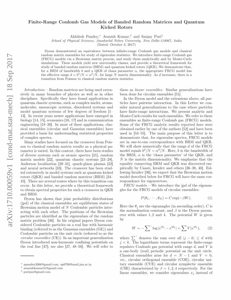
In Fig. 1 we plot p5(s) for d = 2 and β = 1, 2. There isan excellent agreement between the MF approximationand MC numerical results.

The spacing variance is given by

σ2(n− 1) = nξ−1 + γ(β, d). (17)

The leading term in (17) (i.e., the linear term in n) isdetermined by the MF result (16). The constant termγ(β, d) does not arise in the MF approximation, and ismotivated by our exact d = 2 result below. For d > 2,we estimate this constant from our MC calculations. Tocalculate the number variance, we use (15, 16) to obtainthe Laplace transform of the two-level correlation func-tion R2(s) in (9). We find for α ≥ 0,

1

α−∫ ∞

0

e−αsY2(s)ds = ξξ/[(ξ + α)ξ − ξξ]. (18)

The cluster function Y2 falls off exponentially for all d.

0 5 100

0.1

0.2

0.3MCMF

0 5 10

MCMF

s s

p 5(s)

(a) (b)

d=2, β=1 d=2, β=2

FIG. 1. Spacing density p5(s) for d = 2 for (a) β = 1 and (b)β = 2.

Using (18) we can evaluate the number variance Σ2(r) in(10) as

Σ2(r) = σ2(r − 1) + (ξ2 − 1)/(6ξ2). (19)

Exact results for d = 2.—We now outline a generalframework to obtain exact results for d > 1. For sim-plicity we focus on d = 2. Our solutions are expressed interms of the eigenvalues λµ and eigenfunctions fµ of theintegral equation

∫ ∞

0

e−(2β+1)ssβ(s+ t)βfµ(s)ds = λµfµ(t). (20)

Here µ = 0, 1, · · · , β. (A hermitian form of this equa-tion is used in [55]). We order the eigenvalues as λ0 <λ1 < · · · < λβ . The fµ are polynomials of order β. Thelargest eigenvalue λβ is positive and the correspondingeigenfunction has all positive coefficients. The fµ satisfythe orthonormality relation

∫ ∞

0

e−(2β+1)ssβfµ(s)fν(s)ds = δµν . (21)

By integrating Eq. (6) over intermediate spacings fromsn+1, · · · , sN we find

P(n)2 ∝ exp

(

−(2β + 1)n∑

i=1

si

)

n∏

j=1

sβj

n−1∏

k=1

(sk + sk+1)βG(s1, sn),

(22)

where G is only a function of s1, sn. It can be shown thatG is factorizable as F (s1)F (sn) with F (s) ∝ fβ. Thus

P(n)2 can be written as

P(n)2 (s1, · · · sn) =

1

λn−1β

exp

−(2β + 1)n∑

j=1

sj

×

n∏

j=1

sβj

n−1∏

k=1

(sk + sk+1)βfβ(s1)fβ(sn), (23)

valid for n = 1, 2, 3, · · · . Using Eq. (8) one can obtainpn−1. In particular the nearest-neighbor spacing densityis p0(s) = e−(2β+1)ssβ(fβ(s))

2.

4

Integrating Eq. (23) over all variables except s1 and snwe find the jpd of s1 and sn for n > 1,

Qn(s1, sn) = e−(2β+1)(s1+sn)sβ1 sβnfβ(s1)fβ(sn)

β∑

µ=0

(λµ

λβ)n−1fµ(s1)fµ(sn). (24)

Using Eq. (24) the covariance between s1 and sn is givenby

〈s1sn〉 − 1 =

β−1∑

µ=0

(

λµ

λβ

)n−1

〈sfβfµ〉2, (25)

and hence the spacing variance can be shown to be

σ2(n− 1) = n

[

〈s2f2β〉 − 1 + 2

β−1∑

µ=0

(

λµ

λβ − λµ

)

〈sfβfµ〉2]

− 2

β−1∑

µ=0

λµλβ

(λβ − λµ)2〈sfβfµ〉2

[

1−(

λµ

λβ

)n]

. (26)

Here the angular brackets represent

〈F (s)〉 =∫ ∞

0

e−(2β+1)ssβF (s)ds. (27)

The term (λµ/λβ)n

on the right hand side of (26) decaysexponentially yielding (17) with ξ = 2β + 1.

For β = 1 we can obtain the analytic solution of theintegral equation (20). The two eigenvalues and eigen-functions are given respectively by (µ = 0, 1),

λµ =

(

1±√

3

2

)

2

27, fµ(s) =

(

s±√

23

)

√

2|λµ|√

23

, (28)

where + and − correspond to µ = 1, 0 respectively. Using(25, 27) we obtain (18) with γ(1, 2) = 1/18. For β =2, 4, numerical integrations yield γ = 0.045157, 0.030598respectively.

Cases with d > 2.—The integral equation (20) can begeneralized for d > 2, and has ζ+1 eigenvalues and eigen-functions, where ζ = β(d− 1). However the calculationsbecome less tractable for larger d, and we use MC calcula-tions to obtain a complete picture for arbitrary d. Theseresults are shown in Fig. 2, 3. As d increases, there is across-over to the classical ensemble results. For example,for Σ2(r), the classical ensemble results are obtained forr ≪ d.

BRM and QKR.—First we introduce QKR whichhave been studied extensively as model systems ofquantum chaos. Following Izrailev [34], we consideran N -dimensional matrix model for QKR. The evolu-tion operator is given by U = BG, where B(α) =exp [−iα cos(ϕ+ ϕ0)/~], and G = exp

[

−i(p+ γ)2/2~]

.

Here ϕ and p are the position and momentum opera-tors. Further α is the kicking parameter, ϕ0 is the parity-breaking parameter and γ is the time-reversal-breakingparameter. In the position representation

Umn =1

Nexp

[

−iα cos

(

2πm

N+ ϕ0

)]

×

N ′

∑

l=−N ′

exp

[

−i

(

l2

2− γl − 2πµl

N

)]

, (29)

where µ = m − n;m,n = −N ′,−N ′ + 1, · · · , N ′;N ′ =(N − 1)/2. For large α the eigenvalue spectra of U accu-rately exhibit classical ensemble fluctuations (e.g., spac-ing distribution, number variance etc.). These are char-acteristic of the β = 1 case for γ = 0 and the β = 2 casefor γ 6= 0, both with ϕ0 not equal to zero. For our nu-merical simulations we choose ϕ0 = π/2N and γ = 0, 0.7,the latter respectively for β = 1, 2.

Next we consider BRM ensembles {A} of bandwidth bas mentioned above. The jpd of the matrix distributionis P (A) ∝ exp(−trA2/4v2) with v2 being the variance ofthe non-zero off-diagonal matrix elements. As in Eq. (3)we consider a banded matrix A such that the only non-zero elements Ajk arise for |j − k| ≤ b. The matrices arereal-symmetric, complex hermitian and quaternion realself-dual for β = 1, 2, 4 respectively. These ensembleshave semicircular density for b ≫ 1 [22, 39, 43]:

ρ(x) = 2√

R2 − x2/πR2, R2 = 8βbv2. (30)

It has been shown [36–38, 40], that BRM and QKR givethe same nearest-neighbor spacing density p0(s) whenb2/N and α2/N are equal. One of the central resultsof this Letter is that BRM and QKR can be modeled byFRCG with d = b2/N = α2/N for all fluctuation mea-sures. This is confirmed by our numerical results. As dincreases, there is a transition from the Poisson ensembleto the classical ensembles.

Generalizations to non-integer d.—Our FRCG mod-els above correspond to the case of integer d. To coverthe entire parameter range we also introduce FRCG withnon-integer d. In this case we generalize FRCG by mod-ifying (2) so that (6) becomes

Pd = Cδ(

N∑

i=1

si −N)

N∏

j=1

[d]∏

k=0

(sj + · · ·+ sj+k)β∆(k), (31)

where [d] is the largest integer ≤ d. Moreover, ∆(k) = 1for k = 0, 1, · · · , [d]− 1, and ∆([d]) = d− [d].

Numerical results.—We have performed extensive MCsimulations of the FRCG, as well as simulations of BRMand QKR. We show representative numerical results here.For the MC calculations, N = 1000 and data is averagedover 1000 independent runs. Calculations for BRM andQKR are based on a single realization with N = 10000and 5000 respectively. The values of b and α are chosen tobe

√Nd. We have performed calculations for many val-

ues of d including the non-integer cases (not shown here).

5

2 40

0.3

0.6

0.9 BRMQKR

MC/THEORY

2 4

2 40

0.3

0.6

0.9

2 4

5 100

0.2

0.4

5 10

5 100

0.2

0.4

0.6

5 10

p 0(s)

p 0(s)

p 5(s)

p 5(s)

s s

(a) (b)

(c) (d)

(e) (f)

(g) (h)

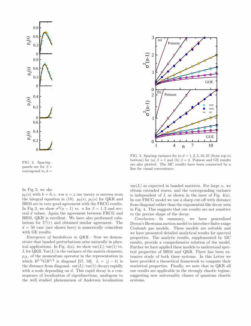
FIG. 2. Spacing density pk(s) for k = 0, 5: Left and rightpanels are for β = 1 and β = 2 respectively. (a), (b), (e), (f)correspond to d = 2; (c), (d), (g), (h) correspond to d = 5.

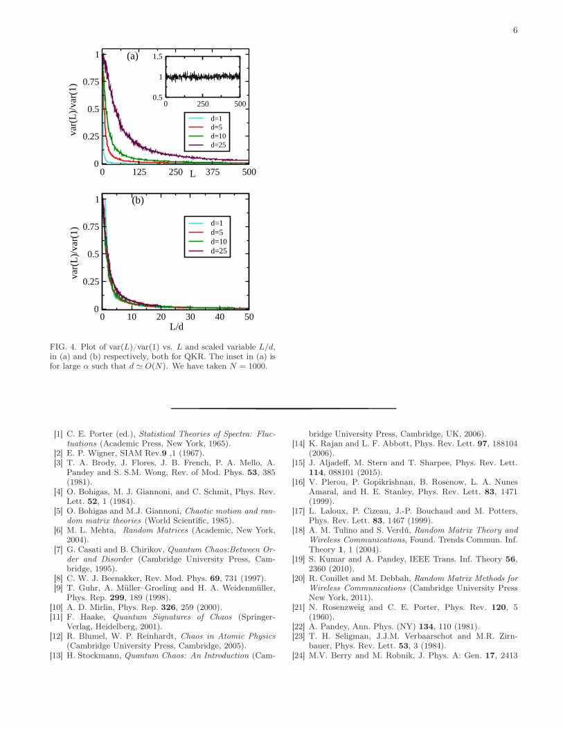
In Fig 2, we show results for β = 1, 2 and d = 2, 5 forpk(s) with k = 0, 5. For d = 2 the theory is derived fromthe integral equation in (18). p0(s), p5(s) for QKR andBRM are in very good agreement with the FRCG results.In Fig 3, we show σ2(n − 1) vs. n for β = 1, 2 and sev-eral d values. Again the agreement between FRCG andBRM, QKR is excellent. We have also performed calu-lations for Σ2(r) and obtained similar agreement. Thed = 50 case (not shown here) is numerically coincidentwith GE results.

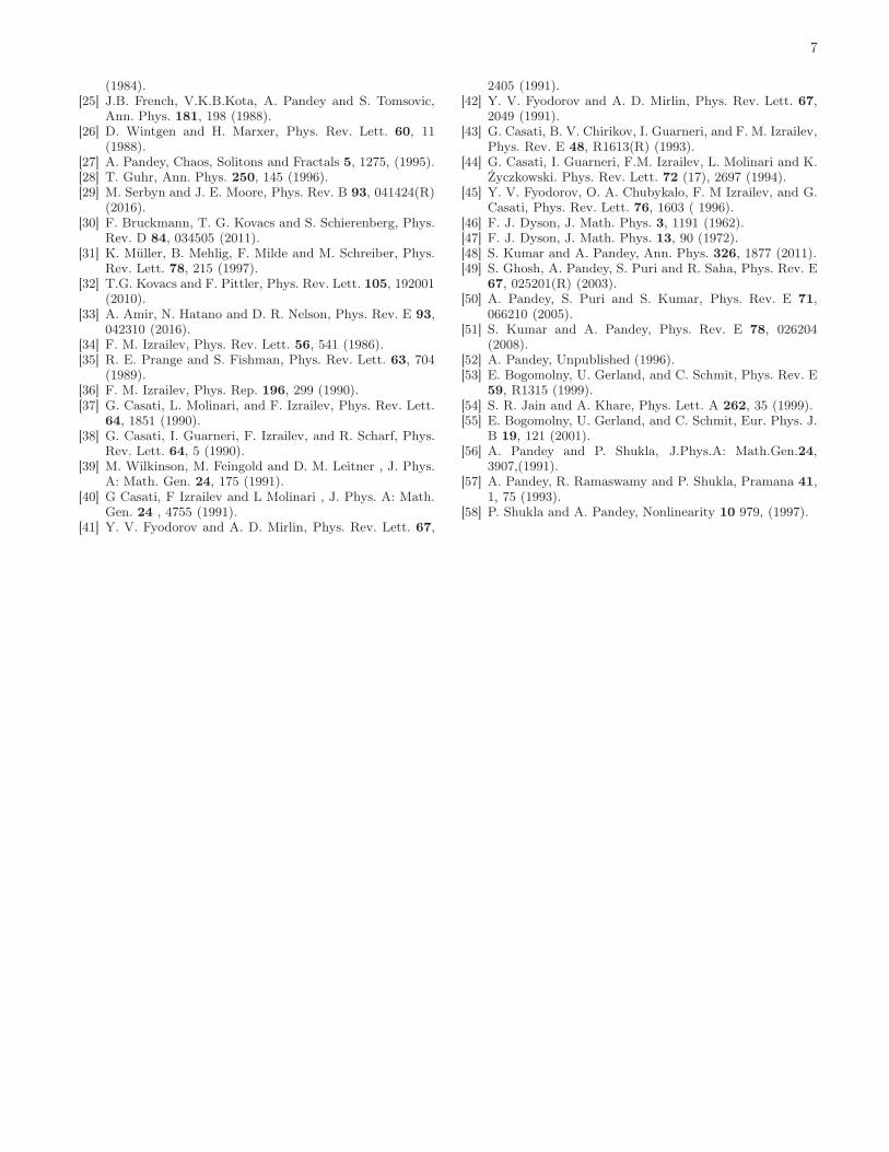
Emergence of bandedness in QKR.—Now we demon-strate that banded perturbations arise naturally in phys-ical applications. In Fig. 4(a), we show var(L)/var(1) vs.L for QKR. Var(L) is the variance of the matrix elements,pjk, of the momentum operator in the representation in

which B1/2GB1/2 is diagonal [57, 58]. L = |j − k| isthe distance from diagonal. var(L)/var(1) decays rapidlywith a scale depending on d. This rapid decay is a con-sequence of localization of eigenfunctions, analogous tothe well studied phenomenon of Anderson localization

[35, 37, 38]. In Fig. 4(b), we show the same quantityplotted against L/d. The excellent data collapse demon-strates that d constitutes a natural scale for the decay of

0

1

2

3

1 4 7 100

1

2

QKR

BRM

MC

Poisson

Poisson

GUE

GOE

σ2 (n-1

)σ2 (n

-1)

(a)

(b)

n

FIG. 3. Spacing variance for to d = 1, 2, 5, 10, 25 (from top tobottom) for (a) β = 1 and (b) β = 2. Poisson and GE resultsare also plotted. The MC results have been connected by aline for visual convenience.

var(L) as expected in banded matrices. For large α, weobtain extended states, and the corresponding varianceis independent of L as shown in the inset of Fig. 4(a).In our FRCG model we use a sharp cut-off with distancefrom diagonal rather than the exponential-like decay seenin Fig. 4. This suggests that our results are not sensitiveto the precise shape of the decay.

Conclusion.—In summary, we have generalizedDyson’s Brownian motion model to introduce finite-rangeCoulomb gas models. These models are solvable andwe have presented detailed analytical results for spectralproperties. The analytic results, supplemented by MCresults, provide a comprehensive solution of the model.Further we have applied these models to understand spec-tral properties of BRM and QKR. There has been ex-tensive study of both these systems. In this Letter wehave provided a theoretical framework to compute theirstatistical properties. Finally, we note that in QKR allour results are applicable in the strongly chaotic regime,suggesting new universality classes of quantum chaoticsystems.

6

0 125 250 375 5000

0.25

0.5

0.75

1

d=1d=5d=10d=25

0 10 20 30 40 500

0.25

0.5

0.75

1

d=1d=5d=10d=25

0 250 5000.5

1

1.5

L

L/d

var(

L)/

var(

1)va

r(L

)/va

r(1)

(a)

(b)

FIG. 4. Plot of var(L)/var(1) vs. L and scaled variable L/d,in (a) and (b) respectively, both for QKR. The inset in (a) isfor large α such that d ≃ O(N). We have taken N = 1000.

[1] C. E. Porter (ed.), Statistical Theories of Spectra: Fluc-

tuations (Academic Press, New York, 1965).[2] E. P. Wigner, SIAM Rev.9 ,1 (1967).[3] T. A. Brody, J. Flores, J. B. French, P. A. Mello, A.

Pandey and S. S.M. Wong, Rev. of Mod. Phys. 53, 385(1981).

[4] O. Bohigas, M. J. Giannoni, and C. Schmit, Phys. Rev.Lett. 52, 1 (1984).

[5] O. Bohigas and M.J. Giannoni, Chaotic motion and ran-

dom matrix theories (World Scientific, 1985).[6] M. L. Mehta, Random Matrices (Academic, New York,

2004).[7] G. Casati and B. Chirikov, Quantum Chaos:Between Or-

der and Disorder (Cambridge University Press, Cam-bridge, 1995).

[8] C. W. J. Beenakker, Rev. Mod. Phys. 69, 731 (1997).[9] T. Guhr, A. Müller–Groeling and H. A. Weidenmüller,

Phys. Rep. 299, 189 (1998).[10] A. D. Mirlin, Phys. Rep. 326, 259 (2000).[11] F. Haake, Quantum Signatures of Chaos (Springer-

Verlag, Heidelberg, 2001).[12] R. Blumel, W. P. Reinhardt, Chaos in Atomic Physics

(Cambridge University Press, Cambridge, 2005).[13] H. Stockmann, Quantum Chaos: An Introduction (Cam-

bridge University Press, Cambridge, UK, 2006).[14] K. Rajan and L. F. Abbott, Phys. Rev. Lett. 97, 188104

(2006).[15] J. Aljadeff, M. Stern and T. Sharpee, Phys. Rev. Lett.

114, 088101 (2015).[16] V. Plerou, P. Gopikrishnan, B. Rosenow, L. A. Nunes

Amaral, and H. E. Stanley, Phys. Rev. Lett. 83, 1471(1999).

[17] L. Laloux, P. Cizeau, J.-P. Bouchaud and M. Potters,Phys. Rev. Lett. 83, 1467 (1999).

[18] A. M. Tulino and S. Verdú, Random Matrix Theory and

Wireless Communications, Found. Trends Commun. Inf.Theory 1, 1 (2004).

[19] S. Kumar and A. Pandey, IEEE Trans. Inf. Theory 56,2360 (2010).

[20] R. Couillet and M. Debbah, Random Matrix Methods for

Wireless Communications (Cambridge University PressNew York, 2011).

[21] N. Rosenzweig and C. E. Porter, Phys. Rev. 120, 5(1960).

[22] A. Pandey, Ann. Phys. (NY) 134, 110 (1981).[23] T. H. Seligman, J.J.M. Verbaarschot and M.R. Zirn-

bauer, Phys. Rev. Lett. 53, 3 (1984).[24] M.V. Berry and M. Robnik, J. Phys. A: Gen. 17, 2413

7

(1984).[25] J.B. French, V.K.B.Kota, A. Pandey and S. Tomsovic,

Ann. Phys. 181, 198 (1988).[26] D. Wintgen and H. Marxer, Phys. Rev. Lett. 60, 11

(1988).[27] A. Pandey, Chaos, Solitons and Fractals 5, 1275, (1995).[28] T. Guhr, Ann. Phys. 250, 145 (1996).[29] M. Serbyn and J. E. Moore, Phys. Rev. B 93, 041424(R)

(2016).[30] F. Bruckmann, T. G. Kovacs and S. Schierenberg, Phys.

Rev. D 84, 034505 (2011).[31] K. Müller, B. Mehlig, F. Milde and M. Schreiber, Phys.

Rev. Lett. 78, 215 (1997).[32] T.G. Kovacs and F. Pittler, Phys. Rev. Lett. 105, 192001

(2010).[33] A. Amir, N. Hatano and D. R. Nelson, Phys. Rev. E 93,

042310 (2016).[34] F. M. Izrailev, Phys. Rev. Lett. 56, 541 (1986).[35] R. E. Prange and S. Fishman, Phys. Rev. Lett. 63, 704

(1989).[36] F. M. Izrailev, Phys. Rep. 196, 299 (1990).[37] G. Casati, L. Molinari, and F. Izrailev, Phys. Rev. Lett.

64, 1851 (1990).[38] G. Casati, I. Guarneri, F. Izrailev, and R. Scharf, Phys.

Rev. Lett. 64, 5 (1990).[39] M. Wilkinson, M. Feingold and D. M. Leitner , J. Phys.

A: Math. Gen. 24, 175 (1991).[40] G Casati, F Izrailev and L Molinari , J. Phys. A: Math.

Gen. 24 , 4755 (1991).[41] Y. V. Fyodorov and A. D. Mirlin, Phys. Rev. Lett. 67,

2405 (1991).[42] Y. V. Fyodorov and A. D. Mirlin, Phys. Rev. Lett. 67,

2049 (1991).[43] G. Casati, B. V. Chirikov, I. Guarneri, and F. M. Izrailev,

Phys. Rev. E 48, R1613(R) (1993).[44] G. Casati, I. Guarneri, F.M. Izrailev, L. Molinari and K.

Życzkowski. Phys. Rev. Lett. 72 (17), 2697 (1994).[45] Y. V. Fyodorov, O. A. Chubykalo, F. M Izrailev, and G.

Casati, Phys. Rev. Lett. 76, 1603 ( 1996).[46] F. J. Dyson, J. Math. Phys. 3, 1191 (1962).[47] F. J. Dyson, J. Math. Phys. 13, 90 (1972).[48] S. Kumar and A. Pandey, Ann. Phys. 326, 1877 (2011).[49] S. Ghosh, A. Pandey, S. Puri and R. Saha, Phys. Rev. E

67, 025201(R) (2003).[50] A. Pandey, S. Puri and S. Kumar, Phys. Rev. E 71,

066210 (2005).[51] S. Kumar and A. Pandey, Phys. Rev. E 78, 026204

(2008).[52] A. Pandey, Unpublished (1996).[53] E. Bogomolny, U. Gerland, and C. Schmit, Phys. Rev. E

59, R1315 (1999).[54] S. R. Jain and A. Khare, Phys. Lett. A 262, 35 (1999).[55] E. Bogomolny, U. Gerland, and C. Schmit, Eur. Phys. J.

B 19, 121 (2001).[56] A. Pandey and P. Shukla, J.Phys.A: Math.Gen.24,

3907,(1991).[57] A. Pandey, R. Ramaswamy and P. Shukla, Pramana 41,

1, 75 (1993).[58] P. Shukla and A. Pandey, Nonlinearity 10 979, (1997).