Mechanisms of chaos in the forced NLS equation

Eli ShlizermanVered Rom-Kedar

Weizmann Institute of Science

eli.shlizerman@weizmann.ac.il

http://www.wisdom.weizmann.ac.il/~elis/

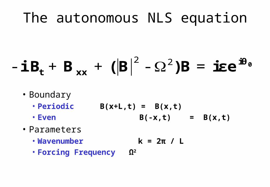
The autonomous NLS equation

0iθxxt eεiB)B(BiB =-++- 22

• Boundary • Periodic B(x+L,t) = B(x,t)• Even B(-x,t) = B(x,t)

• Parameters• Wavenumber k = 2π / L • Forcing Frequency Ω2

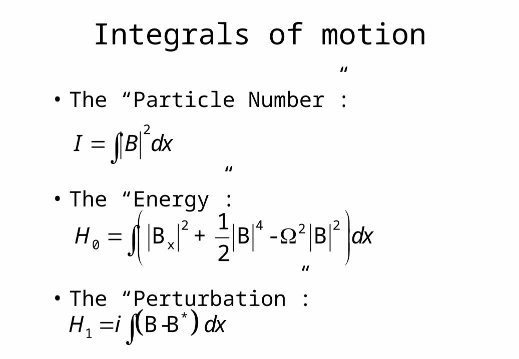
Integrals of motion

• The “Particle Number”:

• The “Energy”:

• The “Perturbation”:

2I B dx

2 4 220 x

1B + B - B

2 H dx

*1 B-B H i dx

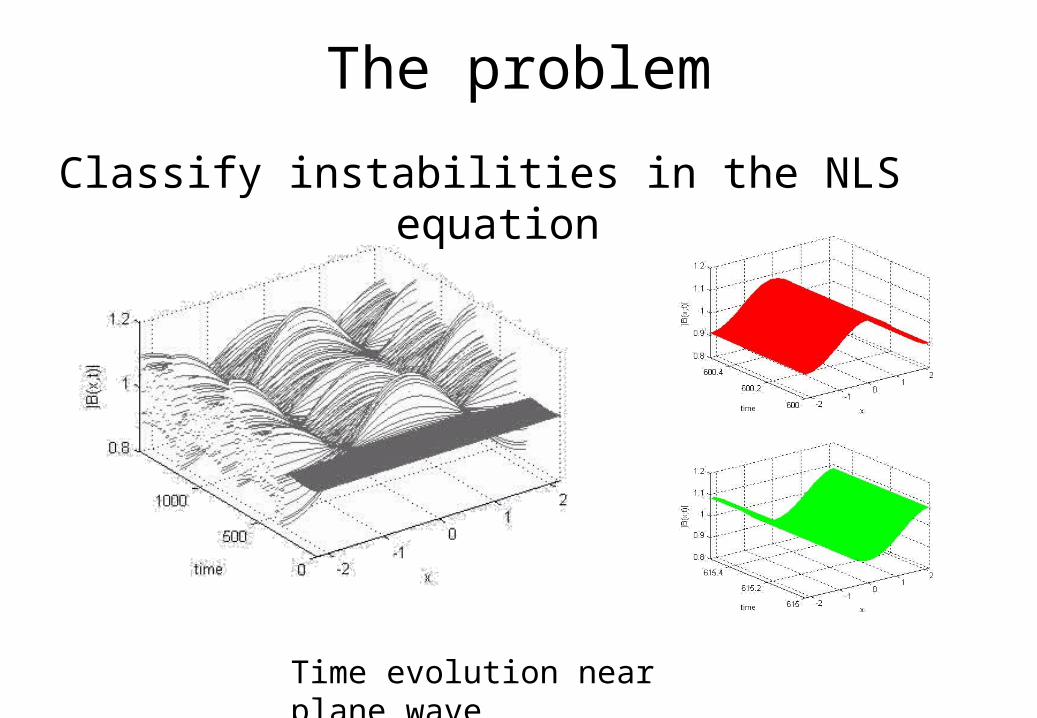
The problem

Classify instabilities in the NLS equation

Time evolution near plane wave

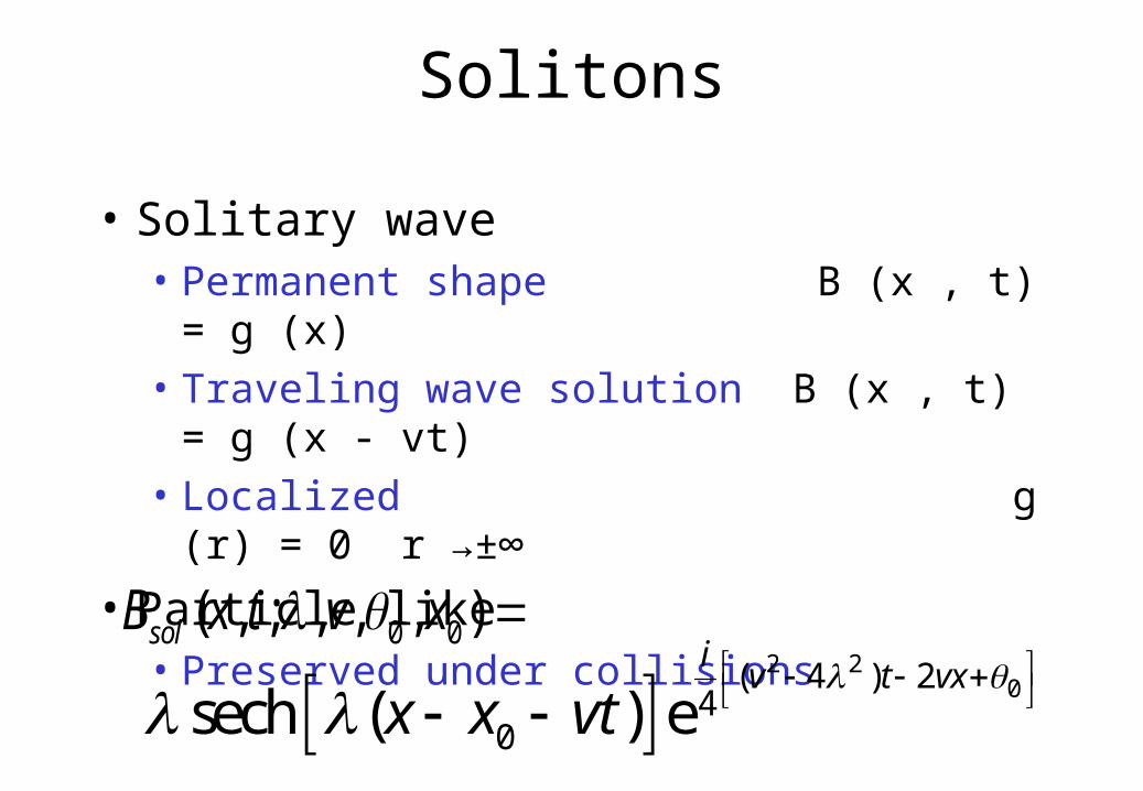
Solitons

• Solitary wave• Permanent shape B (x , t) = g (x)• Traveling wave solution B (x , t) = g (x - vt)• Localized g (r) = 0 r →±∞

• Particle like• Preserved under collisions

0 0( , ; , , , ) solB x t v x

2 2

0( 4 ) 24

0sech ( ) e iv t vx

x x vt

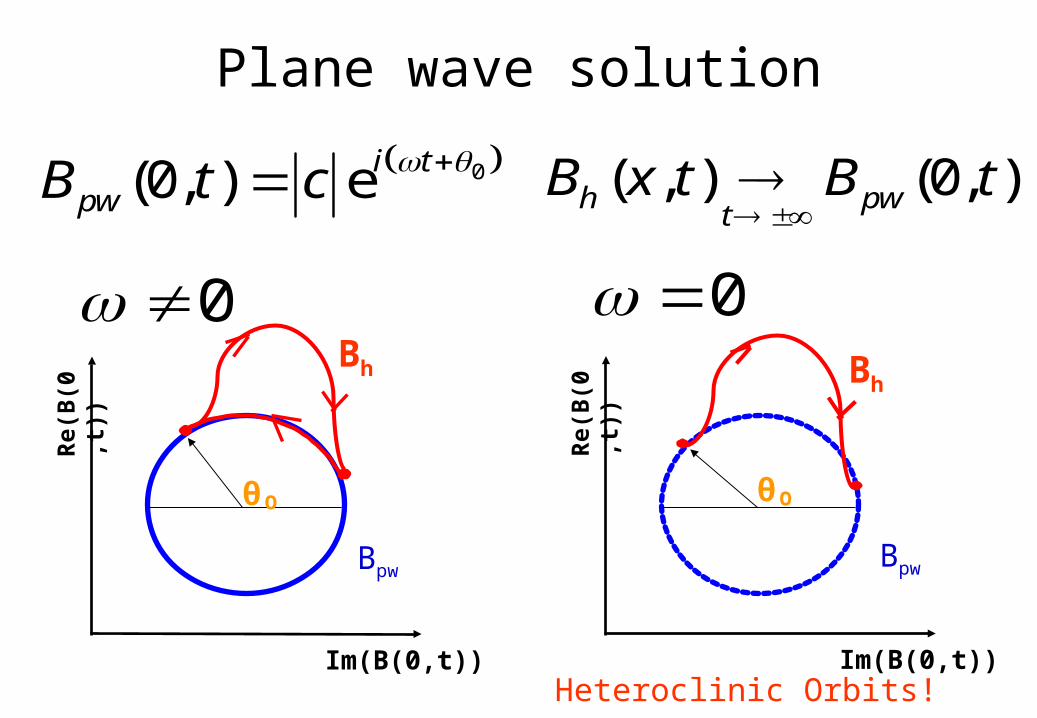
Plane wave solution

Im(B(0,t))

Re(

B(0

,t))

θ₀

Bh

Bpw

Im(B(0,t))

Re(

B(0

,t))

θ₀

Bh

Bpw

Heteroclinic Orbits!

0 0

0(0, ) e i tpwB t c ( , ) (0, )

h pwt

B x t B t

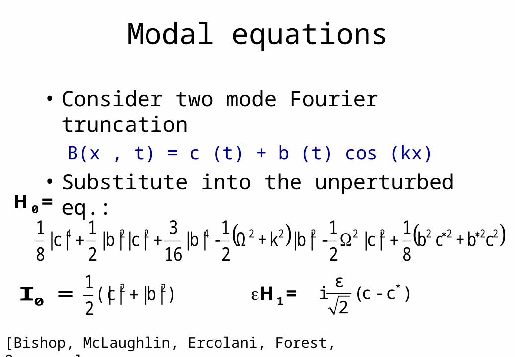
Modal equations

• Consider two mode Fourier truncation B(x , t) = c (t) + b (t) cos (kx)

• Substitute into the unperturbed eq.:

2222222224224 cb+c b8

1 |c|

2

1-|b|k+Ω

2

1-|b|

16

3|c||b|

2

1|c|

8

1

0H =

0I = )|b||c(|2

1 22 *εi (c - c )2

1H =

[Bishop, McLaughlin, Ercolani, Forest, Overmann]

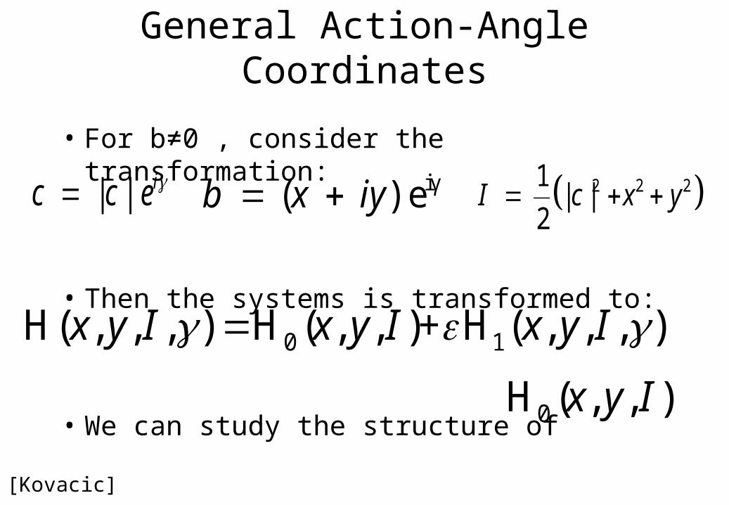
General Action-Angle Coordinates

• For b≠0 , consider the transformation:

• Then the systems is transformed to:

• We can study the structure of

| | ic c e iγ ( ) e b x iy 2 2 21 | |

2 I c x y

0 1H( , , , ) H ( , , )+ H ( , , , )x y I x y I x y I

0H ( , , )x y I

[Kovacic]

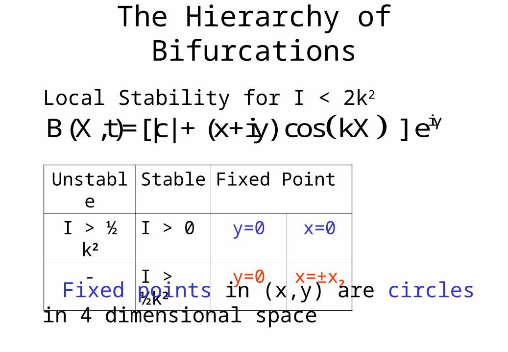
The Hierarchy of Bifurcations

Local Stability for I < 2k2

Fixed Point StableUnstable

x=0y=0I > 0I > ½ k2

x=±x2y=0I > ½k2-

iγB(X,t)=[|c| + (x+iy) cos kX ] e

Fixed points in (x,y) are circles in 4 dimensional space

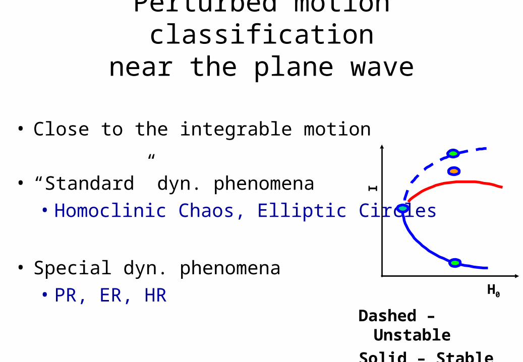
Perturbed motion classificationnear the plane wave

• Close to the integrable motion

• “Standard” dyn. phenomena• Homoclinic Chaos, Elliptic Circles

• Special dyn. phenomena• PR, ER, HR H0

I

Dashed – Unstable

Solid – Stable

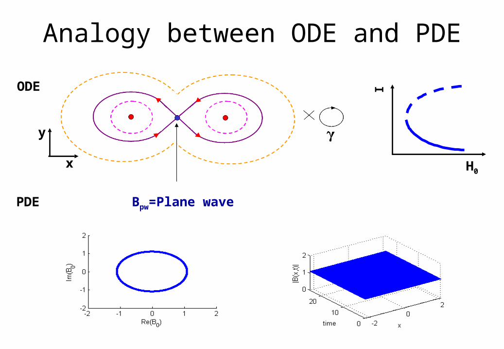
Analogy between ODE and PDE

Bpw=Plane wave

x

y

H0

IODE

PDE

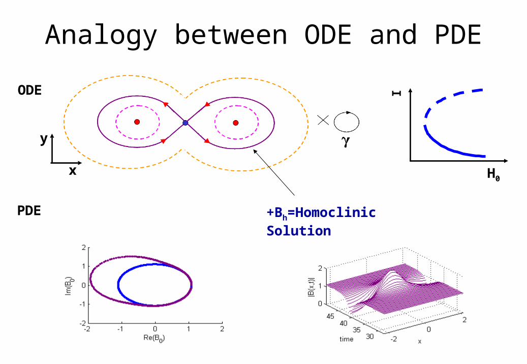
Analogy between ODE and PDE

+Bh=Homoclinic Solution

x

y

H0

IODE

PDE

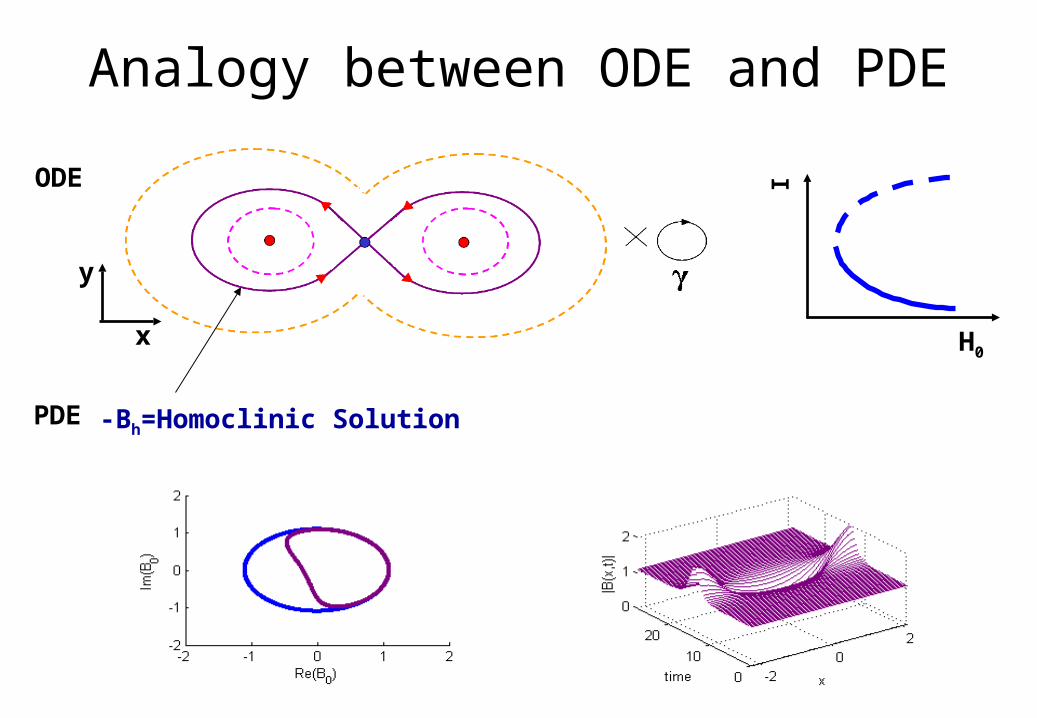
Analogy between ODE and PDE

-Bh=Homoclinic Solution

x

y

H0

IODE

PDE

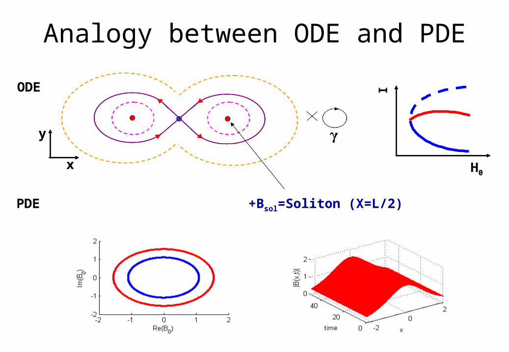
Analogy between ODE and PDE

x

y

H0

IODE

PDE +Bsol=Soliton (X=L/2)

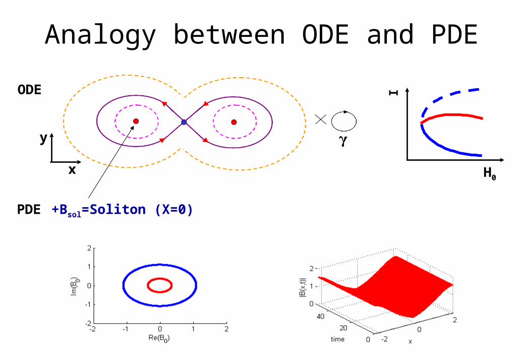
Analogy between ODE and PDE

+Bsol=Soliton (X=0)

x

y

H0

IODE

PDE

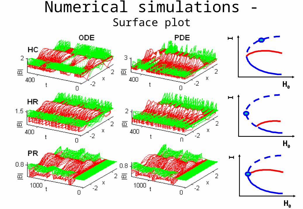
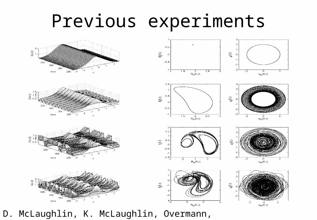
Numerical simulations - Surface plot

H0

I

H0

I

H0

I

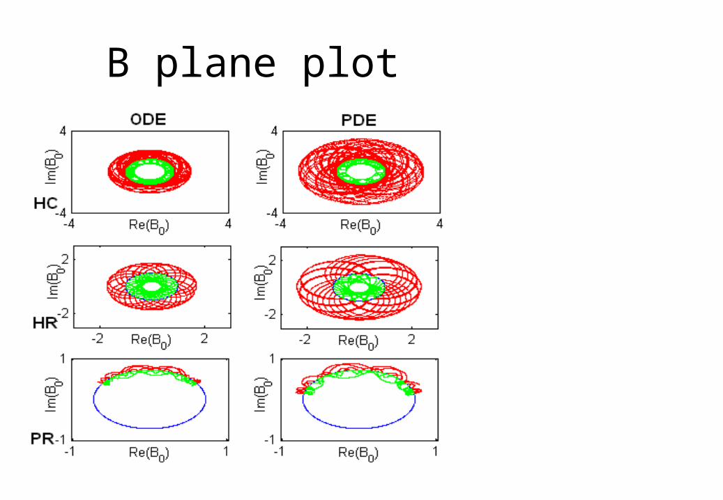
B plane plot

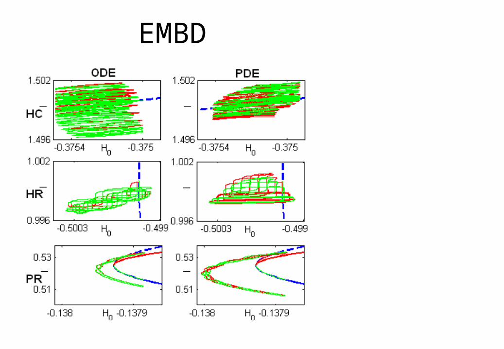
EMBD

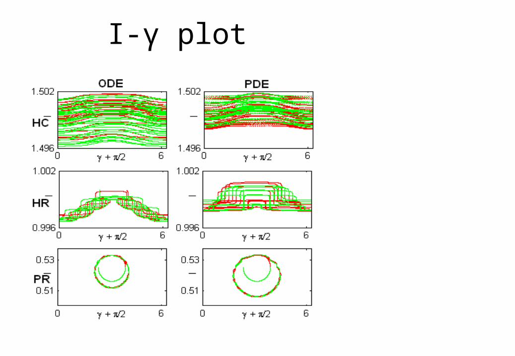
I-γ plot

Conclusions

• Three different types of chaotic behavior and instabilities in Hamiltonian perturbations of the NLS are described.

• The study reveals a new type of behavior near the plane wave solution: Parabolic Resonance.

• Possible applications to Bose-Einstein condensate.

Characterization Tool

• An input: Bin(x,t) – can we place this solution within our classification?

• Quantitative way for classification (tool/measure)HC - O(ε), HR - O(ε1/2), PR - O(ε1/3)

• Applying measure to PDE results

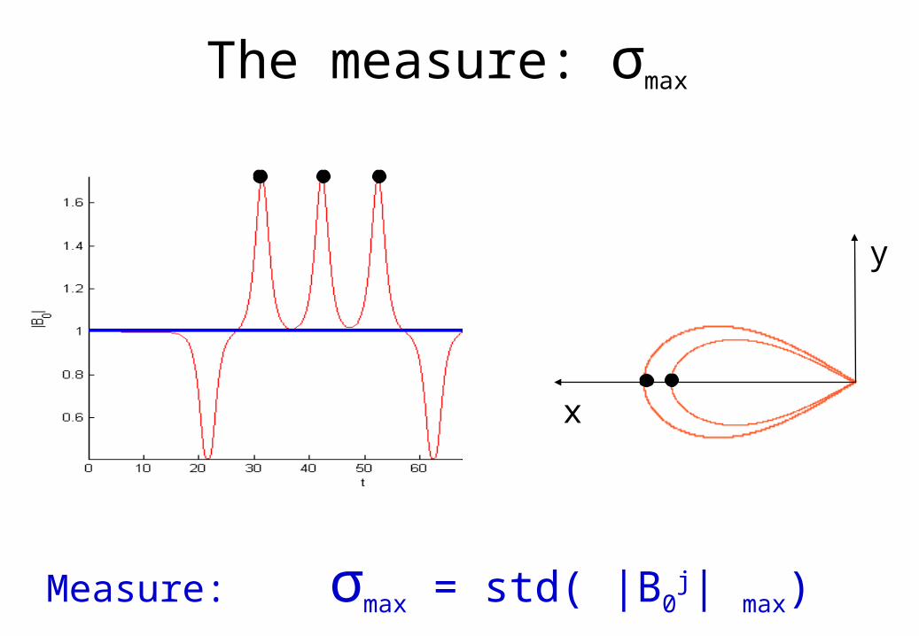
The measure: σmax

x

y

Measure: σmax = std( |B0j| max)

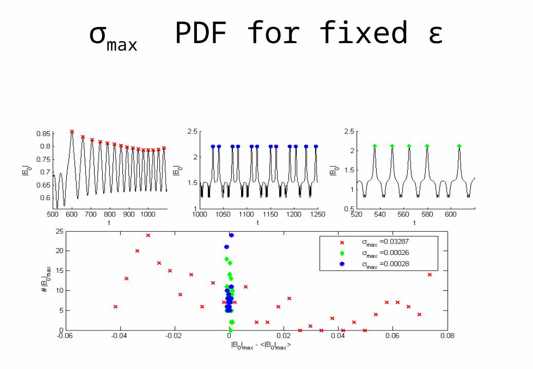
σmax PDF for fixed ε

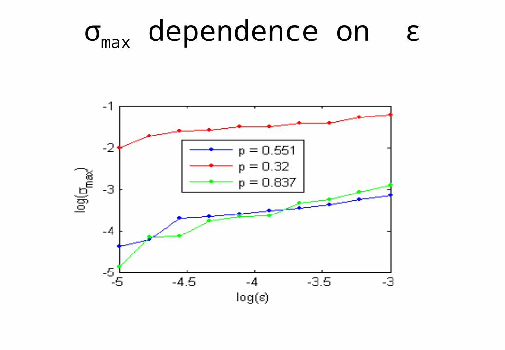
σmax dependence on ε

Future Work

• Capturing the system into PR by variation of the forcing

• Instabilities in the BEC

• Resonant surface waves

Thank you!

Summary

• We analyzed the modal equations with the “Hierarchy of Bifurcations”

• Established the analogy between ODE and PDE

• Numerical simulations of instabilities

• Characterization tool

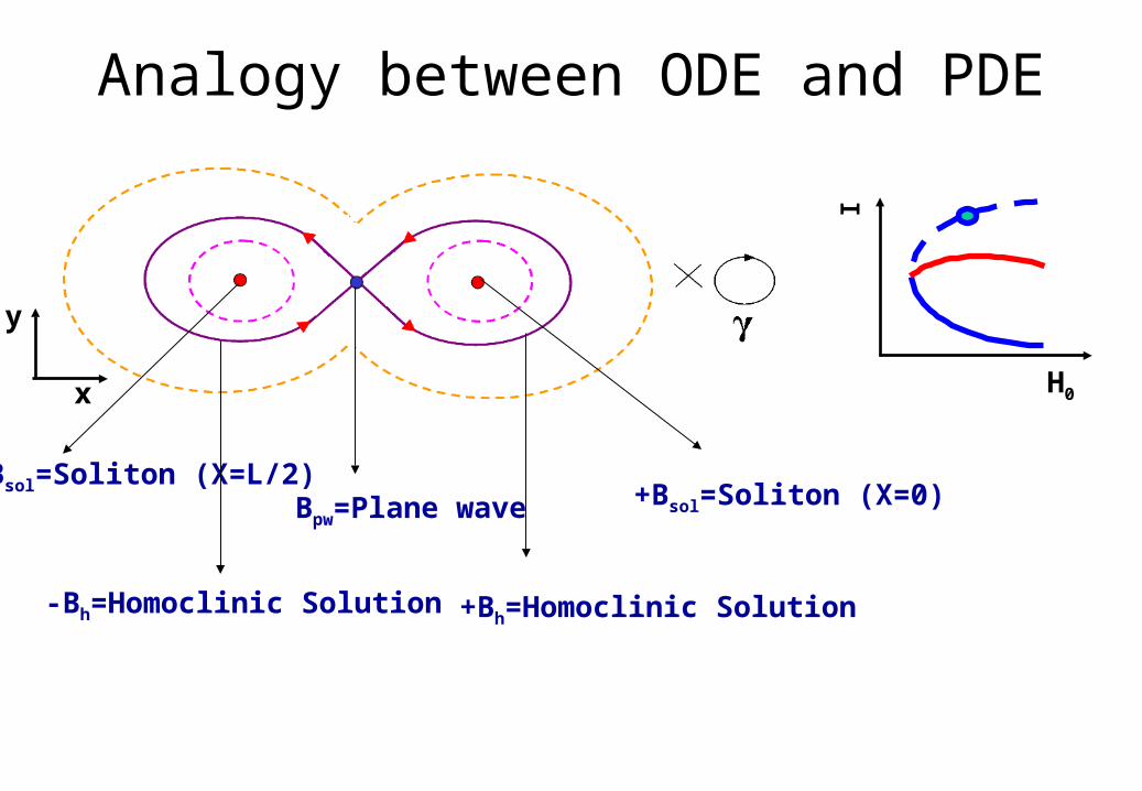
Analogy between ODE and PDE

Bpw=Plane wave +Bsol=Soliton (X=0)

+Bh=Homoclinic Solution

-Bsol=Soliton (X=L/2)

-Bh=Homoclinic Solution

x

y

H0

I

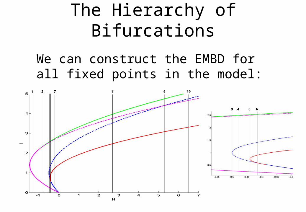
The Hierarchy of Bifurcations

We can construct the EMBD for all fixed points in the model:

D. McLaughlin, K. McLaughlin, Overmann, Cai

Previous experiments

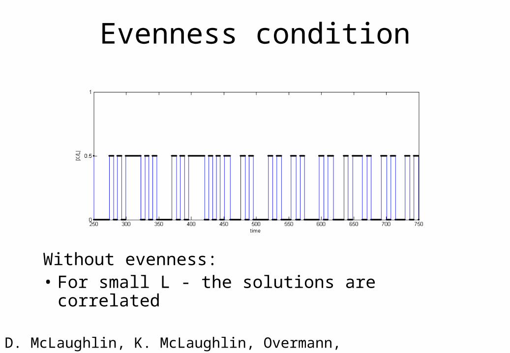
Evenness condition

Without evenness:• For small L - the solutions are correlated

D. McLaughlin, K. McLaughlin, Overmann, Cai

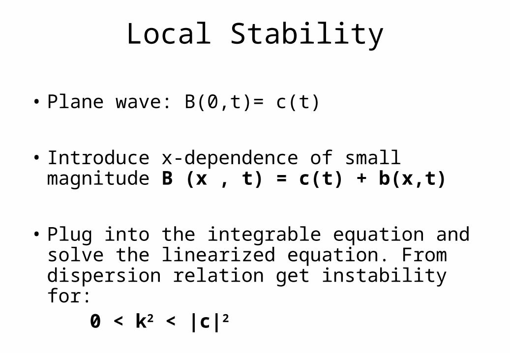
Local Stability

• Plane wave: B(0,t)= c(t)

• Introduce x-dependence of small magnitude B (x , t) = c(t) + b(x,t)

• Plug into the integrable equation and solve the linearized equation. From dispersion relation get instability for:

0 < k2 < |c|2

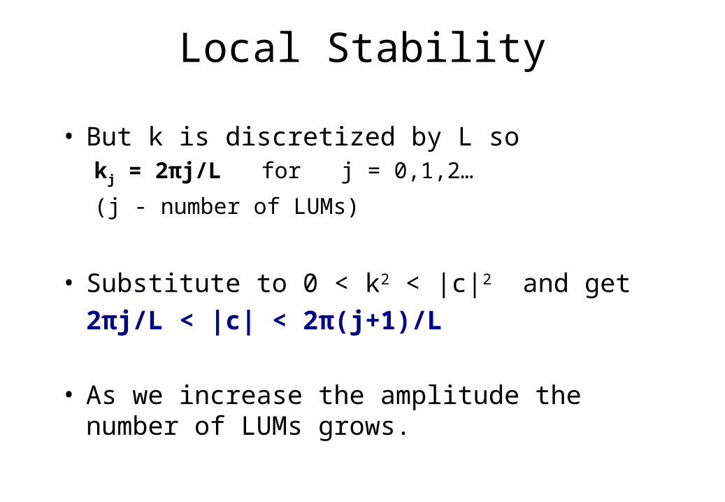
Local Stability

• But k is discretized by L so kj = 2πj/L for j = 0,1,2…

(j - number of LUMs)

• Substitute to 0 < k2 < |c|2 and get

2πj/L < |c| < 2π(j+1)/L

• As we increase the amplitude the number of

LUMs grows.

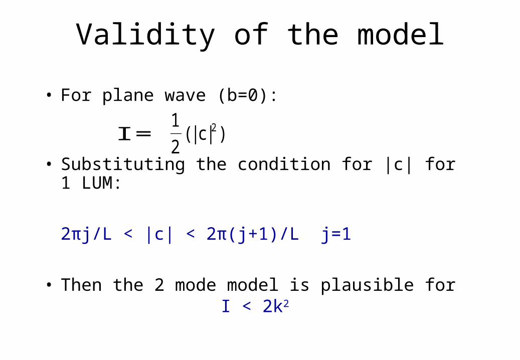
Validity of the model

• For plane wave (b=0):

• Substituting the condition for |c| for 1 LUM:

2πj/L < |c| < 2π(j+1)/L j=1

• Then the 2 mode model is plausible for I < 2k2

I = 21(|c| )

2

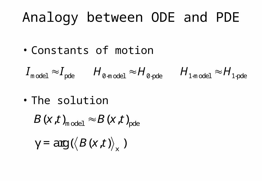
Analogy between ODE and PDE

• Constants of motion

• The solution

model pdeI I 0-model 0-pdeH H 1-model 1-pdeH H

model pde( , ) ( , )B x t B x t

xγ = arg( ( , ) )B x t