
Joint determination of the strong coupling constant and of ...
57
Corso di Laurea Triennale in Fisica Joint determination of the strong coupling constant α s and of the partonic structure of the nucleon. Relatore Interno: Prof. S. Forte Correlatore : Dott. J. Rojo Tesi di Laurea di Simone Lionetti matr. 724668 Anno Accademico 2009-2010
Transcript of Joint determination of the strong coupling constant and of ...
Corso di Laurea Triennale in Fisica
Joint determination of the strong coupling constant αs
and of the partonic structure of the nucleon.
Relatore Interno: Prof. S. Forte
Correlatore : Dott. J. Rojo
Tesi di Laurea diSimone Lionetti
matr. 724668
Anno Accademico 2009-2010

Contents
General introduction v
1 The Structure of the Nucleon 11.1 Deep Inelastic Scattering experiments . . . . . . . . . . . . . . . . . . 11.2 Incoherent interaction and scaling . . . . . . . . . . . . . . . . . . . . 31.3 The parton model . . . . . . . . . . . . . . . . . . . . . . . . . . . . . 41.4 Quarks and confinement . . . . . . . . . . . . . . . . . . . . . . . . . 61.5 Quantum chromodynamics . . . . . . . . . . . . . . . . . . . . . . . . 7
2 The NNPDF approach to global parton fits 112.1 The ideas of NNPDF . . . . . . . . . . . . . . . . . . . . . . . . . . . 112.2 NNPDF versions and data sets . . . . . . . . . . . . . . . . . . . . . 13
3 Statistical treatment of fluctuations 153.1 The χ2 function and the origin of the fluctuations . . . . . . . . . . . 153.2 The three points method . . . . . . . . . . . . . . . . . . . . . . . . . 173.3 Simulating the process to obtain distributions . . . . . . . . . . . . . 213.4 Results . . . . . . . . . . . . . . . . . . . . . . . . . . . . . . . . . . . 23
4 Determination of the strong coupling constant 314.1 A new look on NNPDF 1.2 data . . . . . . . . . . . . . . . . . . . . . 314.2 A DIS-only parton fit with NNPDF2.0 . . . . . . . . . . . . . . . . . 354.3 Results including Drell-Yan, vector boson and jet experiments . . . . 394.4 Variations with the number of replicas . . . . . . . . . . . . . . . . . 44
5 Conclusions and outlook 47

iv CONTENTS
General introduction
One of the most fascinating branches of physics is the chapter of this science whichaims at understanding the features of the microscopic world. This field has led tomany of the most fundamental discoveries that mankind has achieved throughoutits history: let us think of how much knowing about molecules, atoms or electronshas changed life during the last century, in both its practical and speculative sides.
We could say that the first revolution in the direction of studying the structureof matter was made when the first microscope was used to see objects and processeswhich presented the observer with a new phenomenology. Nevertheless, ordinarymicroscopes and human eyes have an intrinsic limitation in their potential, justbecause of their use of visible light as a probe. Namely, the problem is that ordinarylight waves are very small compared to the world as we are used to see it, butthey become a mean of investigation far too approximate when studying equallysmall objects. This is the reason why it was necessary to find other probes witha resolution smaller than ordinary light wavelength, which could give informationabout the natural world with extreme spatial accuracy. A simple analogy can bemade in order to understand this point better. Let us think of our microscopicobject as a car, and imagine throwing balls at it from one side as an experiment toinvestigate the car’s features. Even for a blind scientist who knows nothing of the carit would be possible, albeit obviously not easy, to build up the approximate shapeof the car knowing the angles at which many basket balls are bounced off it. If ourcar is the image for an atom, claiming to study the atom with light waves would bequite like trying to understand the shape of the car with balls of the size of a smallmountain. This whole picture has been drawn to recall that the primary functionof particle accelerators is not very different from that of a microscope: they aremeant to throw high-momentum particles (thus small-wavelength probes accordingto quantum mechanics) at objects, in order to understand the main features of thesmallest known constituents of matter.
There is one more face of the problem that the example of the car can help usunderstand in simple terms. When the subnuclear particles, namely the proton andthe neutron, were first observed, it was quite obvious to think about them as a whole,as much as it is natural to think of the car as a single object when we hit it with abasket ball. Of course, there were some hints for the presence of a substructure inthe nucleon: the possibility of classificating particles in multiplets suggested somekind of internal regularity pattern, but few scientists ventured as far as thinking of
vi General introduction
the supposed constituents of observed particles as true physical objects. But theendless pursuit of knowledge which moves the human mind is never satisfied with ascore, it always moves from results to new questions and to the search for answers.Technological improvements provided particle physicists with more refined tools fortheir work, that is higher-energy particles which could be used as precision probesfor the objects they were studying. What took place can be compared to what wouldhappen giving our imaginary scientist, who was throwing basket balls at the car,a gun. Firing bullets at the car and studying their angle of deflection would givehim information not only about the shape of the object under examination, but alsoabout its internal structure. As much as, given the gun, it is possible to distinguishthe collision of a bullet with a rear mirror from that with a tyre, with deep inelasticscattering experiments it was possible for physicists to tell the difference betweencollisions of a probe with different parts of nucleon, which were later called partons.
Thanks to the many experiments which have been set up to investigate the deep-est known nature of our world, the scientific world was able to develop a theory, calledquantum chromodynamics, that actually allows calculations and interpretation ofevents which involve parton interactions. The main force involved in these processesis regarded as a fundamental interaction, goes by the name of strong coupling, andits actual strength is determined by a fundamental constant of nature associated tothe symbol αs. The aim of the present work is precisely to find a value of the strongcoupling constant αs, and the idea behind this determination is extremely simple.The value of the constant assumed to be correct is that which results in the bestagreement among experimental data. More precisely, the constant is regarded asa free parameter and the object that measures data incompatibility, the chi squareχ2 according to the principle of least squares, is computed as a function of this pa-rameter. Coherently with this principle we assume the value of αs which gives theminimum χ2 to be the best estimation for the fundamental constant, and by statis-tical arguments we are able to give boundaries to constrain it inside a well-definedinterval. This operation will be conducted with caution, as the constant studied isextremely important for the determination of observable quantities in many experi-ments currently in progress, it has not a universally accepted value and there is nota common agreement about its experimental uncertainty yet.
This work is organized as follows. In chapter 1 the experimental and theoreticaldevelopments which have allowed today’s model of the nucleon are summarized, ina brief overview that covers the fundamental concepts of quantum chromodynamics.The attention is focused on deep inelastic scattering experiments, which build up agreat part of our data set, and on the determination of parton distribution functions,that is one of the aims of the present paper. Chapter 2 looks into the procedurechosen to obtain parton distribution functions, as well as in the empirical sourcesat the basis of our analysis. In the following section we discuss the strategy appliedto obtain our estimation of the strong coupling constant and we assess the problemof interpolating a point set with strong random fluctuations independent for eachdatum. Last chapter deals with results for each considered experimental set, which

vii
we examine highlighting differences an studying procedural uncertainties.

viii General introduction
Chapter 1
The Structure of the Nucleon
1.1 Deep Inelastic Scattering experiments
In the field of particle physics, most of the available empirical information comesfrom scattering experiments. The purpose of such physical experiences is to studythe properties of particles through detailed analisys of their collisions. Practicallyspeaking, there are two ways of obtaining this results: in fixed target experimentsone beam of particles is accelerated and pointed against a target which is at rest inthe laboratory frame, while in collider experiments two bunches of particles are bothaccelerated and later thrown one against the other. Though these two ways of settingup the experiment imply totally different problems concerning their realization andeach has its advantages and disadvantages, there is no theoretical difference betweenthe two as long as a change of frame is allowed. For the purpose of the followingdiscussion, it is easier to think of these events in terms of a better known particle,the probe, that hits a fixed target whose properties are to be studied.
The first distinction that must be made is between elastic and inelastic processes.A collision is said to be elastic if the kinetic energy is conserved, meaning it isthe same before and after the collision. Every time this does not happen and thesystem is actually isolated (this is nearly always the case in particle physics), we candeduce that some of the total energy of the system must have changed its shape,from kinetic energy to another form or vice versa. If at least one of the interactingparticles is regarded as having some internal degree of freedom, it may be that somekinetic energy has passed from particle (translational) motion to this hidden store,changing the intrinsic status of the compound object. But if every particle involvedis thought as truly elementary the only way to have a loss or an increase in totalkinetic energy is particle formation or destruction.
Assuming that the initial state of the particles is perfectly known and giventhrough their four-momenta, the final state is constrained by the total four-momentumconservation law, as there are no external forces acting on the system. Thus, of theinitial eight degrees of freedom which characterize the situation after the collision(the eight components of the two four-vectors of the outgoing particles), only four
2 The Structure of the Nucleon
free parameters remain. One of these is the scattering plane angle, which is notessential in order to understand the dynamics of the event. If we assume the probeto be an elementary particle, which is the case for our experiments where leptonsare most commonly used because of their better-known interactions, the mass shellconstrain on the outgoing probe gives another condition leaving only two free pa-rameters. Usually the choice for these two quantities falls upon the energy loss ofthe probe and on the transferred square momentum, which has also an importantphysical interpretation being the norm of the virtual photon four-momentum. Thuswe define
ν = Ef − Ei, Q2 = −q2; (1.1)
where ν is the incident particle energy loss, Ei and Ef are the energies of thesame particle in the initial and final state respectively, q is the force carrier’s four-momentum and Q is a conventional quantity defined in order to avoid dealing withnegative squares. Now, if the scattering is elastic, energy conservation bounds oneof the two parameters and the other describes completely the interaction; namelythe force carrier’s energy always corresponds to the loss of the probe, but it equalsthe kinetic energy of the target after the collision only under the condition providedby elasticity: in this case
ν =Q2
2M, (1.2)
whereM is the mass of the target. In the more interesting case of inelastic scattering,however, no such condition is required; therefore ν and q2 are totally independentvariables.
A leading role in this kind of process is played by the effective area of the targetparticle, which goes by the name of cross section σ; though, the information carriedby this parameter is too approximate and the main observable of scattering exper-iments is usually the differential cross section. The latter is a function of the freeparameters which describe the collision and measures the effective area that resultsin a situation characterized by those parameters. In the case of an inelastic process,for instance, it measures the imaginary surface dσ whose hit results in a final statewith an energy loss of the probe between ν and ν + dν and a momentum transferbetween Q2 and Q2 + dQ2.
Elastic processes, which involve lower energies and are therefore easier to setup, were examined first, and it did not take long for scientists to observe thatexperimental data from this source did not agree with the differential cross sectionformula for Dirac’s point-like particles. Eventually a detailed analysis of elasticscattering led to the conclusion that nucleons had indeed a finite radius. Throughthe measure of the cross section it was possible to parametrize the deviation from thepoint-like behaviour with two functions, named form factors, which were discoveredto be actually the same function and, from a physical point of view, were no otherthan the fourier transform of the proton charge distribution.
1.2 Incoherent interaction and scaling 3
1.2 Incoherent interaction and scaling
γ
e−
N
e−
X
(a) ElectroproductionW+
νµ
N
µ−
X
(b) Neutrinoproduction
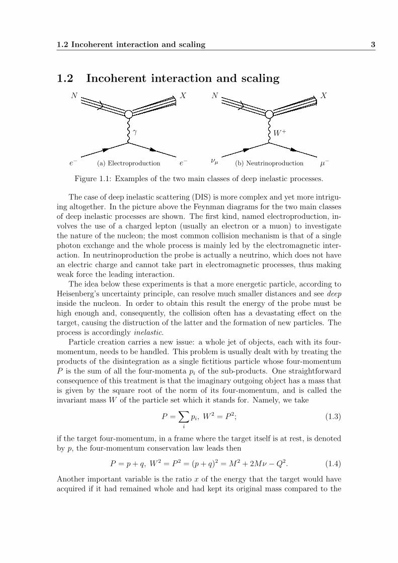
Figure 1.1: Examples of the two main classes of deep inelastic processes.
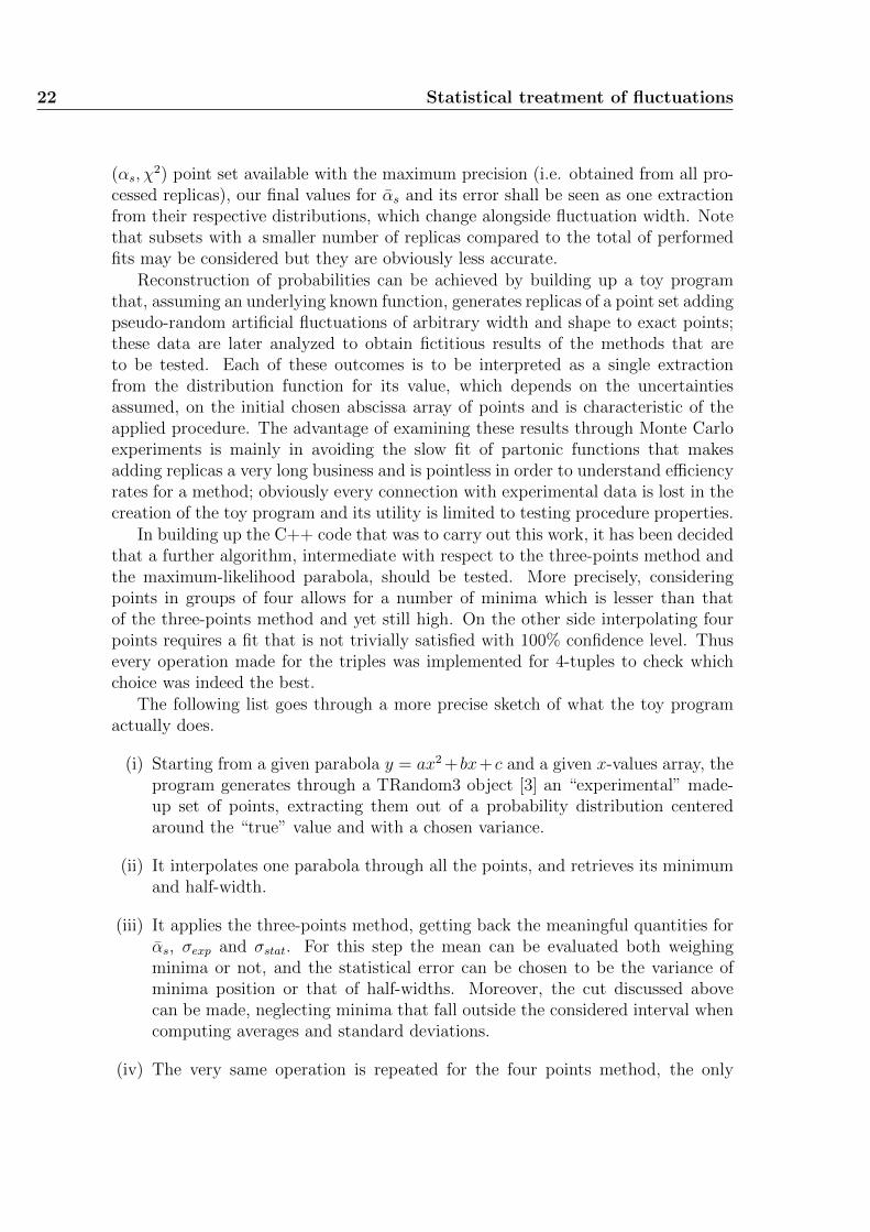
The case of deep inelastic scattering (DIS) is more complex and yet more intrigu-ing altogether. In the picture above the Feynman diagrams for the two main classesof deep inelastic processes are shown. The first kind, named electroproduction, in-volves the use of a charged lepton (usually an electron or a muon) to investigatethe nature of the nucleon; the most common collision mechanism is that of a singlephoton exchange and the whole process is mainly led by the electromagnetic inter-action. In neutrinoproduction the probe is actually a neutrino, which does not havean electric charge and cannot take part in electromagnetic processes, thus makingweak force the leading interaction.
The idea below these experiments is that a more energetic particle, according toHeisenberg’s uncertainty principle, can resolve much smaller distances and see deepinside the nucleon. In order to obtain this result the energy of the probe must behigh enough and, consequently, the collision often has a devastating effect on thetarget, causing the distruction of the latter and the formation of new particles. Theprocess is accordingly inelastic.
Particle creation carries a new issue: a whole jet of objects, each with its four-momentum, needs to be handled. This problem is usually dealt with by treating theproducts of the disintegration as a single fictitious particle whose four-momentumP is the sum of all the four-momenta pi of the sub-products. One straightforwardconsequence of this treatment is that the imaginary outgoing object has a mass thatis given by the square root of the norm of its four-momentum, and is called theinvariant mass W of the particle set which it stands for. Namely, we take
P =∑
i
pi, W2 = P 2; (1.3)
if the target four-momentum, in a frame where the target itself is at rest, is denotedby p, the four-momentum conservation law leads then
P = p+ q, W 2 = P 2 = (p+ q)2 = M2 + 2Mν −Q2. (1.4)
Another important variable is the ratio x of the energy that the target would haveacquired if it had remained whole and had kept its original mass compared to the
4 The Structure of the Nucleon
energy carried by the photon. Hence we define
x =Q2
2Mν, (1.5)
and, as x equals one when energy conservation holds and zero when all the energybrought by the photon results in no momentum transfer, it measures somehow the“elasticity” of the event.
When experimental data became available, it was natural to parametrize theempirical differential cross section with structure functions, which were to play forDIS the role that had been covered by form factors in elastic scattering. Namely, itwas assumed that (
d2σ
dQ2dν
)eN=
4πα2
Q4
EfEi
1
M
[2FE1 (Q2, ν) sin2 ϑ
2+M
νFE2 (Q2, ν) cos2
ϑ
2
], (1.6)(
d2σ
dQ2dν
)νN=G2F
2π
EfEi
[2FW1 (Q2, ν) sin2 ϑ
2+ FW2 (Q2, ν) cos2
ϑ
2± FW3 (Q2, ν)
Ei + EfM
sin2 ϑ
2
], (1.7)
where the first equation is for electromagnetic events and the second refers to weak-interaction-led processes. The trends of FE
1 , FE2 , FW
1 , FW2 and FW
3 were determinedby requiring the relations above to hold.
It was thus found, starting from physical experiences, that the structure func-tions’ dependence on the variables Q2 and ν is extremely simple (as long as thevalues of the two parameters involved are high enough), and that in the case ofcharged lepton - nucleon interaction the two functions are tightly related. As amatter of fact there were theoretical conjectures enough to expect these behaviours.
First of all it must be considered that in the case of elastic scattering the mass ofthe nucleon, which does not change during the interaction, naturally sets a dimen-sional length scale for the reaction, while in DIS there is no quantity to perform thistask. Therefore it is not surprising to find that for high Q2 and high ν the structurefunctions, which are pure numbers, show dependence only on the value of a dimen-sionless combination of the two. The variable x defined as above can be chosen tocover this position, in which case the behaviour that has just been described andgoes under the name of Bjorken scaling can be formally stated as follows:
F1(Q2, ν) = F1(x), F2(Q2, ν) = F2(x). (1.8)
The close relationship between the two functions was the equality that links structurefunctions for spin-1/2 particles, namely
F2(x) = 2xF1(x), (1.9)
and was interpreted as a hint for the existence of fermion constituents.
1.3 The parton model
It has been argued that the lack of a dimensional quantity to set the length scale ofthe reaction shows up in scaling; now we want to show that this property has a more
1.3 The parton model 5
far-reaching physical interpretation, if one is to set up a model to explain the internalstructure of the nucleon. The spatial extent of this particle was revealed by elasticscattering experiments which were able to produce a number for its radius: by meansof the Fourier transform it was possible to find a value of about 0.8 femtometers forthe radius of the sphere representing the proton charge distribution. Neverthelessthe absence of a scale in DIS experiments suggests an interaction of the photonwith a dimensionless, that is point-like, object. Following the path that startsfrom this observation, and making no other assumption, it is possible to develop amodel where an undefined number of point-like particles named partons, carryingunspecified charge and momentum, builds up the nucleon.
A brief but important observation must be made before reaching further con-clusions. Saying that the virtual boson which mediates the interaction between alepton and a nucleon hits a single dimensionless object implies that the object itselfis free on the spacetime scale of the collision, otherwise a third particle bound to thetarget would take part in the event too and this would show in the analysis. Namely,if the time of the electron-parton interaction were large enough to allow interpartoninformation exchange, the struck particle would carry or push away another and theinvolved target would be made of two particles; another length, the mean distance ofthe partons, would then become important and hide the scaling feature. As experi-mental evidence is against this conclusion it must be assumed that, at high energieswhere scaling shows, the virtual boson exchange between the lepton and the struckparton is quick enough to be finished before the other partons become aware thatsomething’s happening. Thus the force that binds partons together, which goes bythe name of strong interaction, slackens asymptotically for small distances and highenergies; this feature is referred to as asymptotic freedom.
Let now fi(x) be the probability distribution function for the i-th parton to carryat a given time t a fraction x of the total four-momentum of the nucleon. Startingfrom these parton distribution functions (PDFs) and from the known expressionsfor the differential cross section of dimensionless particles, it is possible to evalu-ate the cross section of the nucleon both for weak and electromagnetic interaction.Comparing these relations with equations 1.6 and 1.7 it is possible to link structurefunctions to the probabilities fi, and thus to gain information about the nucleonparton composition from experiments. While this comparison operation is carriedout, the argument of the structure functions, which arises naturally in the compu-tation of the cross section and actually happens to be the fraction of momentum xborne by the struck parton, is identified with the scaling variable. Therefore, underthe hypoteses of the parton model, these two quantities coincide and the rudenessof using the same symbol to indicate both up to this point may be forgiven.
Using the tools built together with this model it is possible to extrapolate the con-tents of experimental data from structure functions to PDFs, whose interpretationis much more straightforward. Through processes mediated by the electromagneticforce one may tell apart distribution functions associated with different charges andmagnetic moments, while using the information from neutrino-nucleon scattering
6 The Structure of the Nucleon
matter and antimatter contributions to the total differential cross section can beseparated. The result of this process is a set of PDFs which represent the internalstructure of the nucleon, thought as an object composed of many point-like particles.
1.4 Quarks and confinement
When Feynman and Bjorken came up with this model, there was another field ofresearch in particle physics whose results were immediately related to partons: par-ticle classification. The huge host of different particles which had been discoveredhad called for a logical scheme to organize them, and the search for such a classifica-tion had been answered best by Gell-Mann’s quark model. This phenomenologicaltheory had split the known hadrons into multiplets, and counted on the possibilityof seeing strongly interacting particles as composed of two or three simpler objectsnamed quarks to classify them. By the assumption of the existance of three differentkinds of quarks, or flavours, hadrons were divided into multiplets according to anSU(3) symmetry scheme. The success of this hypotesis was astonishing, especiallyfor people who did not believe in the physical reality of quarks yet. As a matter offact many scientists thought at first that the success of these supposed constituentsof the nucleon was limited to particle classification, but when the parton model wasdeveloped it reminded immediately about quarks.
Nowadays six kinds of quarks have been succesfully observed, coming up in threeisospin doublets very much like leptons.
(ud
) (cs
) (tb
)(1.10)
The six quark flavours (up, down, charm, strange, top, bottom) divided in doublets
As a matter of fact, it seems that every elementary fermion comes in three versions,which can be told apart only because they have different masses. Inside a strongisospin doublet, instead, particles can be distinguished only because of the presenceof the electromagnetic interaction, i.e. they differ because of their charge, and ofnothing else.
According to the quark model every meson is made up of two quarks, while everybaryon, including the nucleons which are the object of this research, is composedby three. Nevertheless, one must not hurry to the conclusion that these contituentsalone account for all the properties of the hadrons, as the presence of other objectsinside of them cannot be ruled out a priori; it was thus very good that in buildingup the parton model no assumption about the number of partons was made.
Particle classification had taught a lot about the quantum numbers (i.e. charges,isospin, baryon number...) of quarks, and it was then straightforward to use this in-formation to determine quark PDFs for the nucleon setting as unknown a probabilityfunction for each light flavour. Through experimental determination of parton dis-tribution functions it was thus confirmed that the momentum fraction carried by up
1.5 Quantum chromodynamics 7
and down quarks in neutrons and protons is in good agreement with the hypotesis ofquark composition made for particle classification, and it was discovered that thereseems to be a small amount of antimatter inside any matter baryon. Nevertheless,though momentum ratios determined through PDFs are in good agreement withpredictions from the quark model, the contributions of the light-flavoured quarksaccount only for half of the total momentum of the nucleon; this has been inter-preted as an evidence for an important presence of uncharged strong-force carriersinside hadrons.
Anyway, what was said leads to the conclusion that the structure of the nucleonis complex, and that the three constituent quarks suggested by the flavour symmetryscheme, sometimes called valence quarks, are but a part of it. Indeed, when a moredetailed analyses is carried out, traces of quark-antiquark pairs from the vacuum sea(known as sea quarks) and strongly-interacting bosons named gluons may be seen.
A last phenomenological observation must be made before venturing in the spec-ulative side of this matter. This is to do with the lack of any evidence for theexistence of fractional electric charges. Even in DIS experiments, where a singleparton is struck hard and gains enough energy to tear the nucleon apart, no hint forthe presence of isolated quarks scattering free after the collision was ever seen: theresult of such an event is rather a jet of other hadrons and, eventually, sub-productssuch as photons or vacuum pairs. The outcomes of the parton model are so goodthat rejecting it just for this, however important, missing proof seems unwise; nev-ertheless the gap created in the theory by such a failure in observations calls for aformal statement. Namely, to save all has been done up till now, we must admitthat quarks exist only inside hadrons, perhaps because they are bound so tightlythat every attempt at pulling them out of bigger particles results in the much lessenergetically expensive production of a quark-antiquark pair. This last feature ofthe strong interaction is referred to as confinement.
1.5 Quantum chromodynamics
Two faults emerged in the SU(3) flavour scheme soon after its conception: one wasthe total emptiness of some multiplets which were not matched by observed particleswhile others were filled perfectly, another was a particle which appeared to violateopenly the Pauli exclusion principle. Let us examine the latter first.
The Gell-Mann theory of quarks provides for the ∆++ resonance particle a quarkcomposition (uuu): this hadron finds its natural location in the spin 3/2 baryonmultiplet as made up of three up quarks. The problem is that the wavefunctionassociated to the given charge and angular momentum must be totally symmetric,whilst it should be anti-symmetric under exchange of any two identical fermions suchas the up-flavoured quarks are; moreover the discovery of the more exotic Ω− = (sss)particle shows that the case is not isolated.
As a mean to escape this self-contradiction the introduction of a new quantum
8 The Structure of the Nucleon
number, later named colour, was suggested: as n different eigenvalues allow theconstruction of a wave function totally antisymmetric for n particles, three differentcolours are enough to successfully perform the trick. This far-fetched hypotesis wasformulated ad hoc, but it gained much more importance because it was directlyconnected to a possible solution of the other mentioned problem.
In fact, the introduction of an observable such as colour allowed a classificationof hadrons in another, different, SU(3) symmetry scheme regardless of any flavourdistinction. The fact that no evidence of a charge such as colour had yet beendiscovered in the known hadrons was a hint to find out that only the combina-tions of quarks which gave birth to a colour singlet had a matching filled flavourmultiplet. Thus it was concluded that only colourless (or, better, colour-balanced)hadrons could exist for a time long enough to allow their observation; the mostsimple combinations of this kind being a quark-antiquark pair and three quarks ofthree different colours. This statement is much more persuasive because it leads tolook at quark confinement as a conclusion rather than a cause: as isolated quarksare not in a colour-singlet state they cannot be free. Because of their colour charge,they need to stay glued to something else to become neutral and are thus confinedinto colour-balanced hadrons. Furthermore, from this point of view the interactionamong nucleons can be seen as a residual of the internal strong-force balancing:no net colour charge gives rise nevertheless to high-order effects which bind thenucleus together. This mechanism reminds very much of the Van der Waals force,which comes out of no net electric charge being generated by dipole and higher-orderelectric moments.
Now, the absence of a clear way to define a particular colour suggests some kindof independence of the strong interaction from the specific chosen colour coding, thatis a symmetry under redefinition of strong charges. The three colours introducedso far can be seen as the fundamental representation of the colour SU(3) symmetrygroup, and the lagrangian of the force due to this new charge may be required to beinvariant under local colour-code redefinition. A new gauge field must then be set upto communicate this convention between different points, and treating such a fieldwith quantum mechanics asks for the introduction of a new boson: the gluon. This isthe mechanism which gives birth to gauge field theories, which has been successfullyapplied to develop quantum electrodynamics (QED) before anything was knownabout colour; when a new source of interaction was discovered it was sort of naturalto hope that the same procedure could be applied again. Today the branch ofphysics that arises when the colour hypotesis becomes a gauge theory, whose nameis quantum chromodynamics and is often shortened as QCD, has improved inasmuchas to enter the field of precision physics.
One of the most fascinating features of gauge theories is the variation of chargeswith the energy involved in the measure process. This can be made clear recallingthat, according to the laws of quantum mechanics, particle pairs can borrow energyfrom the vacuum as long as they exist for a very short time. Let a point-likeelectric charge, for instance, be isolated in the void and probed by an electromagnetic
1.5 Quantum chromodynamics 9
interaction: the particle interacting with the charge can see electron-poistron pairsappear close to the charge and stay there for a little while. As these pairs emergewith no net charge but non-zero dipole momentum, they behave as small electricdipoles, orienting themselves and slightly screening the charge. The smaller thespace resolution of the probe, the less the number of particle pairs it sees betweenitself and the charge: thus the electric charge looks greater when seen at shortdistances. As this behaviour affects all the sources of the considered field, it isusually preferred to think that it is not the charge that changes, but the constantsetting the interaction strength itself. Thus the fine structure “constant” α increaseswith the energy involved in a process, because the screening effect of the vacuumspace decreases.
A similar behaviour is shown by the strong interaction whose relevance changeswith distance, but a radical difference between electromagnetic and colour forcesbecomes apparent when it comes to the trend of the strong coupling constant αs.Indeed while a photon carries no electric charge, and its presence in the vacuum seacan be ignored when it comes to evaluating the shielding effect of charges becauseof the void medium, gluons, according to QCD, come in eight different-colouredversions and can actually interact amongst themselves. The contribution of gluonpairs must then be added to that of quark-antiquark pairs in order to obtain acorrect insight of strong interaction’s intensity variation, and such a factor has ananti-screening effect over colour charges. This process of gluon polarisation prevailsover quark charge-shielding, thus giving the strong force a growing importance forgreater distances. What has just been said is in good agreement with the features ofasymptotic freedom and confinement which have been previously mentioned in theirphenomenological aspects, and leads to consider the parameter αs as a function ofthe length scale. As length quantities are directly linked to energies and then tomasses through the two fundamental constants ~ and c, it is equivalent to expressthis dependence taking mass as a variable instead of length. In order to make thecomparison between values as easy as possible, the most common convention usedtoday is to express the value of αs(m) for m = MZ where MZ is the mass of the Zparticle that has been measured with a very high precision during experiments atthe LEP collider; if data is determined for different mass scales QCD provides thetools to evolve results till their matching MZ-referred values.
It is worth to say that the variation of the strong interaction with energy, andparticularly asymptotic freedom, plays a key role in quantum chromodynamics. In-deed no success in performing any exact QCD calculation has been achieved yet; theonly way to make this theory a fertile ground is to use perturbative techniques in or-der to obtain approximations which can be compared to experimental results. Thismethod may be applied only if a situation where chromodynamic effects are verysmall is found, and asymptotic freedom guarantees that short distance phenomenameet this requirement.
Let us finally relate quantum chromodynamics to a last feature internal structureof the nucleon. When higher precision experiments and larger kinematical ranges
10 The Structure of the Nucleon
were explored it was discovered that scaling as it was described above was only anapproximation. Namely the structure functions show a light dependence on Q2, andso do parton distribution functions: as the momentum transfer increases valencequarks’ PDFs tend to show that these partons carry a lesser fraction of the totalmomentum of the nucleon. This trend is now interpreted as follows. As long as themomentum transfer involved in the process is low, the parton distribution functionsof the valence quarks indicate they bring about one third of the total momentumeach, but the PDFs are already far from being delta-like in x = 1/3 because ofHeisenberg’s uncertainty principle: the quarks are confined inside the nucleus, thus∆q is consequently small and ∆p cannot vanish. When Q2 gets greater, though,the probe starts to see the details of the continuous gluon exchange between valencequarks, and the production of quark-antiquark pairs induced by the presence of thesegluons. The more deeply such mechanisms are seen, the smaller is the momentumfraction which appears to be carried by the three quarks: some momentum willindeed be lent for short times to sea particles or gluon, and show as missing fromvalence quark distributions. Although the brief summary given here is not veryaccurate, this explanation should account for the change of the structure functionswith Q2, which gives rise to scaling violations.
Chapter 2
The NNPDF approach to globalparton fits
2.1 The ideas of NNPDF
The present chapter deals with the procedure used to obtain parton distributionfunctions, data sets employed to achieve their estimations and the key idea thattransforms a parton fit into a tool which allows for a measure of the strong cou-pling together with the PDFs. The first observation that should be made is that,according to what has been previously said, different experiments provide differentinformations about partons, thus in order to produce a detailed PDF set reproducingevery feature of the nucleon structure at its best it is desirable to have as a startingpoint a source as wide and varied as possible. This is the reason of the need forglobal parton fits, whose aim is exactly to build up a single optimal set of partondistribution functions.
The framework of these complex procedures can be summarized as follows. Onone side there is an ensemble of measured observables alongside their experimentaluncertainties, while on the other we have a collection of aspirant parton distributionfunctions with a number of free parameters which describe them. Basically theseparameters are varied following some strategy as to make reconstructed observablesas close to the empirical informations as possible. Building up measurable quantitiesthat can be compared with empirical results out of PDFs is a difficoult business in-volving perturbative QCD calculations, which can be carried out at different orders.
For the purpose of the present work we use an approach named Neural NetworkParton Distribution Functions, often abbreviated as NNPDF, which contemplatesthe usage of redundantly parametrized neural networks as unbiased interpolants.This procedure claims to be capable of a determination of the structure of thenucleon that involves no assumption on the functional form used to represent partondistributions, and to produce a faithful estimate for the uncertainties of its results;moreover it allows for the choice of any value for the strong coupling, which is anecessary requirement to apply the chosen strategy to obtain αs.
12 The NNPDF approach to global parton fits
Giving up any hypotesis on the functional form for the PDFs raises many prob-lems which have a nontrivial solution. Indeed the mechanism that realizes such anachievement is actually the use of a highly flexible function which can manage agood interpolation for almost any point set, regardessly of its features. For thispurpose a neural network with an exceedingly high number of free parameters hasbeen chosen, mainly because of its ability at copying trends without any preferencefor a specific class of functions, e.g. periodic functions or polynomials. The mostrelevant issue is then perhaps the necessity of avoiding a fit process that ends upfollowing, together with the true trend hidden behind empirical results, the randomfluctuations around their actual values, which are an effect of accidental errors. Asthe fitting of a neural network to some data is usually known as training, the situ-ation arising when this danger comes true is referred to as overtraining. A geneticalgorithm is used to search for the best values of the networks’ parameters, andthe mentioned problem is solved by employing a specific stopping criterion for theinterpolation named cross-validation; the latter prescribes to split the esperimentaldata available in two sets and the usage of one for the fit while the other checks theabsence of overtraining. Namely at each step of the fitting process a group of randommodifications for the parameters of the neural network is suggested, observables forall considered experiments are computed according to every new PDF set and thebest move is chosen according to the principle of maximum likelihood, consideringonly the training set. This conotinuous loop is stopped either when the agreementbetween forecasts for validation set observables from the PDFs start getting worse,as this means that accidental errors are being fitted, or when a certain number ofsteps have been made, because it is likely that the fit has already converged anddiscrepancies with the validation points are too small to be seen.
A second chief problem that NNPDF solves with a remarkably ingenious strat-egy is the matter of finding a reliable value for the uncertainties affecting the PDFset. Every available datum used by NNPDF is somewhat more than a single exper-imental point, value and uncertainty, as it comes from many measurements: we canimagine that, to some degree of accuracy, the whole statistical distribution generatedby the experiment is given altogether. Evoluting these probabilities into contoursthat stand for confidence level regions around the PDFs is definitely not an easytask, especially when ascertained that the price paid to obtain unbiased results in-cludes a non-deterministic nature of the interpolation’s outcome. Considered thatfurthermore the PDF set is influenced by theoretical assumptions and starts froma set of experiments that is not wholly self-consistent one may get an idea of theawkwardness of the issue. As a direct propagation of uncertainties from empiri-cal probability density functions is extremely complicated, a different approach toobtain faithful confidence level contours for the PDFs is needed.
Such a strategy is given by seeing data as probability distribution functions ac-cording to the view expressed before: this way it is possible to virtually carry outthe experiments an arbitrary number of times. The information on uncertaintiesis so transferred from a certain probability function p(x1, ..., xn) of obtaining the
2.2 NNPDF versions and data sets 13
observable vector (x1, ..., xn) to a population of vectors which reproduce the orig-inal information as accurately as desired. This mechanism makes creating MonteCarlo copies of the original data set a useful tool: it allows a large-at-will numberof parton set computations, whose many resulting PDFs can be later analized toobtain errors using standard statistical techniques. The variance of the functionsobtained according to this method accounts then for both the experimental errorsand uncertainties due to imperfect fitting.
A detailed analysis of how these concepts were developed, implemented andtested goes beyond the purpose of this work and may be found in references [2] and[1]. Here, however, it is important to underline that the strong coupling constantplays a twofold role in this analysis. First, αs is used to evaluate the mean expectedvalues of observables starting from the parton distribution function set through per-turbative QCD techniques. A second step requiring its estimation is the calculationof kernels which allow to evolve PDFs until the scale of the considered experimentis reached. Provided that in both these points a specific entry for the strong cou-pling is assumed, it is possible to obtain the internal structure of the nucleon for anarbitrary value of αs.
2.2 NNPDF versions and data sets
The analysis made by NNPDF is fully performed at next-to-leading order (NLO)in QCD perturbation theory and contemplates a basis of five to seven functions forthe PDF set (depending on program release), parametrized by the same numberof neural networks with more than one hundred free parameters each. The actualnumber of degrees of freedom is much lower, as so many variables are used toavoid interpolation bias but a much smaller set is indeed required to reproduce thefunctions’ behaviour correctly. Anyway the ensembles of experimental points usedin the present work have at least 2800 measured observables, thus to obtain roughestimations of the difference between the number of data and the number of freeparameters the latter can be neglected.
Versions 1.X of NNPDF consider only DIS experiments as data sources. Moreprecisely, these older fits included informations coming from:
- proton and deuteron structure functions as determined from fixed-target scat-tering experiments, as collected by the NMC and BCDMS collaborations plusa set from SLAC;
- collider experiments carried out by the H1 and ZEUS collaborations (includingthe FLH108 set);
- neutrino and antineutrino scattering data as collected by the CHORUS group.
Because of known problem of systematics of the HERA and ZEUS collections,these informations have been reorganized and recollected in the HERA-I combineddataset which has been employed in NNPDF since version 2.0 was developed.
14 The NNPDF approach to global parton fits
As a matter of fact this version’s improvements include a better treatment ofheavy quark thresholds as well as some changes that make the parton fit faster anmore reliable. The critical leap from releases 1.X to 2.X, however, has been madewhen other classes of experiments were considered together with DIS sources inorder to obtain a more precise estimation. Namely, the new information gatheredcan be divided as follows:
- two series of observable measures, associated to the abbreviations DYE605and DYE806, from Drell-Yan fixed-target experiments;
- some data sets from Tevatron involving vector-boson production, includingCDF and D0 Z rapidity distributions as well as CDF W boson asymmetry;
- information from the second runs of CDF and D0, involving inclusive jet pro-duction.
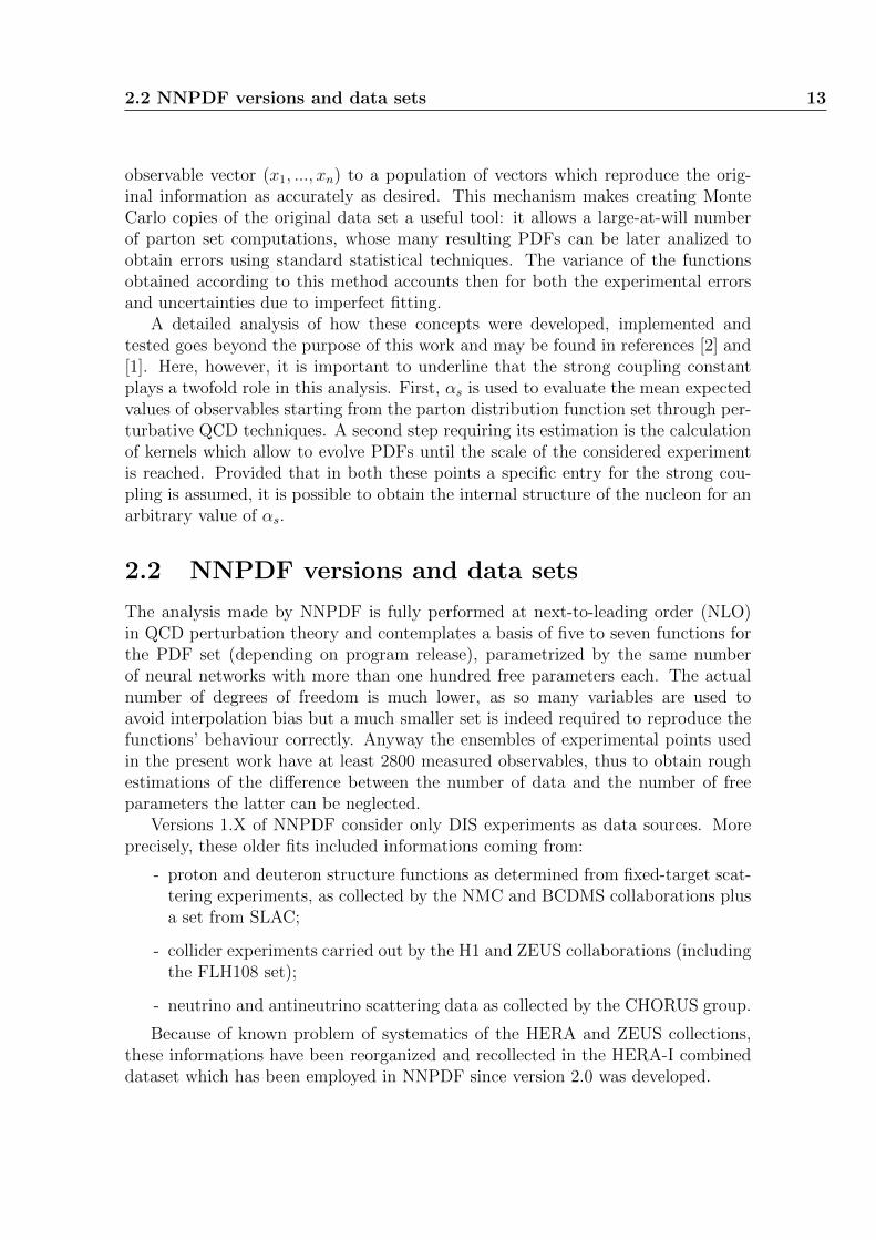
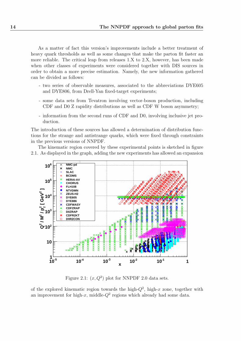
The introduction of these sources has allowed a determination of distribution func-tions for the strange and antistrange quarks, which were fixed through constraintsin the previous versions of NNPDF.
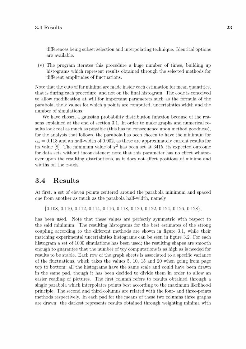
The kinematic region covered by these experimental points is sketched in figure2.1. As displayed in the graph, adding the new experiments has allowed an expansion
x-510 -410 -310 -210 -110 1
]2 [
GeV
2 T /
p2
/ M
2Q
1
10
210
310
410
510
610 NMC-pdNMCSLACBCDMSHERAI-AVCHORUSFLH108NTVDMNZEUS-H2DYE605DYE886CDFWASYCDFZRAPD0ZRAPCDFR2KTD0R2CON
NNPDF2.0 dataset
Figure 1: Experimental data which enter the NNPDF2.0 analysis (Table 1). For hadronic data,the values of x1 and x2 determined by leading order partonic kinematics (Eqs. (3), (4) and (12))are plotted (two values per data point).
computed from the knowledge of statistical, systematic and normalization uncertaintiesas follows:
(covt0)IJ =
(Nc∑
l=1
σI,lσJ,l + δIJσ2I,s
)FIFJ +
(Na∑
n=1
σI,nσJ,n +
Nr∑
n=1
σI,nσJ,n
)F
(0)I F
(0)J , (1)
where I and J run over the experimental points, FI and FJ are the measured central
values for the observables I and J , and F(0)I , F
(0)J are the corresponding observables as
determined from some previous fit.The uncertainties, given as relative values, are: σI,l, the Nc correlated systematic
uncertainties; σI,n, the Na (Nr) absolute (relative) normalization uncertainties; σI,s thestatistical uncertainties (which includes uncorrelated systematic uncertainties). The val-
ues of F(0)I have been determined iteratively, by repeating the fit and using for F
(0)I at each
iteration the results of the previous fit. In practice, convergence of the procedure is very
fast and the final values of F(0)I used in Eq. (1) do not differ significantly from the final
NNPDF2.0 fit results. Note that thanks to this iterative procedure, normalization uncer-tainties can be included in the covariance matrix as all other systematics and thereforethey do not require the fitting of shift parameters.
7
Figure 2.1: (x,Q2) plot for NNPDF 2.0 data sets.
of the explored kinematic region towards the high-Q2, high-x zone, together withan improvement for high-x, middle-Q2 regions which already had some data.
Chapter 3
Statistical treatment offluctuations
3.1 The χ2 function and the origin of the fluctua-
tions
Chances of improving physical knowledge are often, if not always, tightly related tothe possibility of finding laws which agree with experimental data. A quantitativeparameter to objectively measure discrepancies is then needed, and by acceptingthe principle of least squares the natural choice befalls upon the χ2 function. If themost likely rule that fits experimental data is to be determined by decreasing thesquare distances of phenomenological values from law predictions as far as possible,the function which measures the sums of these squares gains a favored role. Theunit to measure a square distance properly is given by the uncertainty that affectsthe experimental point; thus the correct expression of the χ2 function is
χ2 = (xi − fi(k)) Σ−1ij (xj − fj(k)); (3.1)
where Σij is the covariance matrix for the experimental values xi, and fi(k) is thevector of expected values for observables given the set of parameters k whose accordwith empirical data is to be found.
Usually to get the best possible law which rules the trend of experimental dataa class of simple enough functions is chosen, depending on one or more parameters,and the χ2 application is then minimized upon the whole space of allowed values forthose parameters. In our case the situation is only slightly different. Indeed, findingout the correct values for neural networks is not trivial as overtraining must beavoided; moreover, alongside the very high, indeed redundant, number of parametersfor each parton distribution function, we have the degree of freedom provided by αs.Thus we actually constrain one parameter, the strong coupling constant, to assumea certain value, limiting the allowed domain for variables to a submanifold of theoriginal space, and we minimize the χ2 inside that hypersurface. By repeating this
16 Statistical treatment of fluctuations
operation for each foil of the original manifold, we would obtain a one-dimensionalsubset where the minimum is found for sure. As it is impossible to perform thesubmanifold minimization infinite times, we are satisfied by doing it for a largeenough number of αs values: assuming smoothness for the function χ2(αs), its firstderivative in the minimum point αs vanishes. It is likely (and altogether requestedby theoretical arguments) to find a non-zero second derivative in the same point,thus the function, according to Taylor’s theorem, should be well approximated bya parabola in some neighbourhood of αs. Note that it is impossible to foretellwhich the said neighbourhood may be, and the answer depends on the precisionrequired as well. Only a posteriori data analysis will accept or reject the hypotesisabout nonvanishing second derivative and detect an interval where the parabolaapproximation is good enough.
Besides, by statistical arguments [5], it is possible to show that the 68% con-fidence interval for a single underlying parameter determined as explained abovecorresponds to the x-axis span determined through the condition ∆χ2 = 1: thisproperty shall be used to evaluate error bars for αs due to experimental uncer-tainties. When reading the following sections, always keep in mind that the widthof the parabola which approximates the graph of χ2(αs) around its minimum is aproperty of the experimental data: if no other problem affected our analysis, theparabola would provide a single exact location for the minimum point and a definitewidth at ∆χ2 = 1, which could be read as the most likely value and its uncertaintyaccording to the sources of information. The purpose of our fit for χ2(αs), whichhas to deal with non-trivial complications which cloud data properties, is to recoverthese straightforward quantities as accurately as possible. Therefore, we would likeprocedure and statistical errors to be small, possibly negligible, while we want toascertain the right value for the physical uncertainty of the result.
Stepping backwards a little, let us recall that the agreement between a certainnumber n of multigaussian-distributed measures and the value predicted for them bya functional form with m parameters fitted according to the principle of maximumlikelihood has a probability distribution function given by
fd(z) =1
2d/2Γ(d/2)zd2−1e−
z2 , z ∈ [0,+∞); (3.2)
for producing a certain chi square value z, where d = n−m. Evaluating mean andvariance for this function one finds that, for a single fit, the expected value for χ2 isgiven by d and its standard deviation equals
√2d.
In an ideal scheme of our situation, for every Monte Carlo copy of the originaldata set a perfectly performed fit would result in a different χ2 value, that corre-sponds to a single extraction from the probability function above. Adding replicaswould allow an increasingly better sight of parton distributions and their errors, aswell as an improvement in the knowledge of the χ2 distribution function. As themean value of a distribution is estimated with an uncertainty equal to that of thedistribution itself divided by the square root of the number of extractions, the mean
3.2 The three points method 17
χ2 would be determined with a standard deviation of
σ =
√2d
Nrep
; (3.3)
where d is the number of degrees of freedom in the fit and Nrep is the number ofreplicas used.
However, the NNPDF strategy to ascertain the best interpolating PDFs is notfaultless: three main error sources arise as a consequence of the adopted procedure.The first is about our data sets. Indeed, though there is no single experimentexplicitly clashing with all the others, we have evidence for a certain residual internaldata inconsistency of some experiments (again, see [2]). The second problem consistsin theoretical hypoteses which are assumed when it comes to the determination ofparton distribution functions and observable reconstruction. Positivity constraintsand NLO approximations are two examples of these conjectures which may welldisagree with experimental informations. The third and last element which maycause variations in the χ2 distribution function is the imperfection of the stoppingalgorithm, which has been improved much in passing from release 1.2 of NNPDFto 2.0 but cannot boast to be perfect yet. If this feature is examined togetherwith the casual nature of the genetic algorithm employed, it becomes clear thatthe same artificial point set can produce different replicas for parton distributionfunctions. Nevertheless, while the two former problems are systematics that cannotbe addressed by any mean other than changing data sets and theoretical constraints,the last issue can be solved to some extent by adding replicas and averaging them.
Therefore another source of accidental uncertainty affects our chi square, makingstatistical error bars grow larger than σ and altering the shape of the probabilityfunction above. Because we believe the two effects - probability width and fit uncer-tainty - to be of comparable importance, we shall assume the fluctuations of χ2 areapproximately gaussian as it usually happens for uncertainties coming out of morethan one contribution.
3.2 The three points method
Considered the existence of fluctuations and the functional form for χ2(αs), themost obvious thing to do would be to fit through the available points a parabolaaccording to the principle of least squares, i.e. looking for the one that results inthe minimum χ2. However determining uncertainties for the pairs (αs, χ
2) resultingfrom replica analysis is not an easy business; thus some way to proceed withouterror bars is needed. Moreover the formula 3.3, though approximated, shows thatfor few replicas the fluctuations around the mean value of χ2 are large. This isfound to make the minimum obtained through a single interpolating parabola veryunreliable. Thus, at the beginning of any analysis, finding out if everything is goingas expected is a hard business.
18 Statistical treatment of fluctuations
A suggestion to develop a more stable technique has been made in reference [7],observing that some information about resulting minimum reliability is enclosed inthe Np fluctuating points (αs, χ
2). If the chi square mean values had null uncertainty,the latter could be perfectly set on a parabola and any combination of three pointswould be sufficient for a perfect determination of the minimum. The central idea isthen that the population of all the minima obtained through considering each subsetof three points can give an estimation of how much χ2 fluctuations can alter results.It seems that, as a greater population clearly provides better information, the choiceof three as the number of elements in these subsets should be the best: two pointsare not enough to build a unique parabola with an unspecified vertical symmetryaxis, while going for larger subsets of Ns elements would result in a smaller numberof minima, as this is given by
Nmin =
(Np
Ns
). (3.4)
Let us now analize the starting situation and build up the whole procedure. UsingNNPDF the whole experimental data set is copied a certain number of times and foreach copy a global parton fit is carried out, later obtaining the best estimation PDFset as an average of many replicas and finally its corresponding chi square value.Note that the χ2 map 3.1 depends explicitly on the considered data set, and so doesits minimum; indeed considering only a part of the original data is mathematicallytranslated into extracting a sub-vector and a sub-matrix, and this gives rise to adifferent function. Therefore, even if the program performing the global fit gives backa χ2 value for each experiment, this is not expected to be the quantity needed to findthe best-fitting parameter αs for that specific experiment. This should be clear bylooking back at submanifolds: if in each foil a point is chosen by the criterion for thewhole data, the resulting curve obtained does not generally include the minimumin the whole submanifold for a different function. Again, changing the chosen valuefor the strong coupling constant NNPDF may find suitable to worsen the agreementfor a specific experiment, if one or more others make up for this worsening with abetter fit. The goodness of fit obtained for each experiment is then only a measureof how well it is reproduced by the global fit and future considerations about partialchi square should be seen as purely heuristic.
Suppose now that a number of (αs, χ2) couples have been determined, the fol-
lowing steps show their analysis in detail.
(i) For each possible unordered triple of points, say
(αj, χ
2j
), j = 1, 2, 3; (3.5)
a parabola of the form y = aix2 + bix+ ci is interpolated by solving the linear
system
χ21 = ai α
21 + bi α1 + ci
χ22 = ai α
22 + bi α2 + ci
χ23 = ai α
23 + bi α3 + ci
(3.6)
3.2 The three points method 19
in the unknowns ai, bi and ci (the index i cycles on every three-points combi-nation). The minimum is then given by
αi = − bi2ai
. (3.7)
(ii) The uncertainty range for the estimated value αi due to experimental sourcesis evaluated as the inverse image of the ordinate axis interval which goes fromthe minimum χ2 to χ2 + ∆χ2, where ∆χ2 = 1. Accordingly we obtain theintersections between the parabola and the line y = χ2
i + ∆χ2 by requiring
aix2 + bix+ ci = χ2
i + ∆χ2, (3.8)
where
χ2i = aiα
2i + biαi + ci. (3.9)
Hence, solving equation 3.8, computing the difference between the solutionsand dividing by two, the parabola halfwidth that stands for empirical standarddeviation is recovered
σi =
√b2i − 4ai (ci − χ2
i −∆χ2)
2ai. (3.10)
(iii) It may happen that because of strong fluctuations some of the parabolae in-terpolating a triple of points actually curve downwards; thus they have only amaximum instead of a minimum. We have decided that extrema of this natureshould be totally ignored when using this method, because they detect a quan-tity which clearly does not correspond to the one we are looking for. Naturallysuch a choice is fully justified only when the triples discarded because of thisreason are a very small ratio of the whole, otherwise the presence of manymaxima suggests that fluctuations are wide enough as to make this procedurenot faithful. The expected value for αs is then taken as the mean of all theactual minima αi: said M the subset of the indexes 1, ..., Nmin that standfor true minima and |M | its cardinality, we have
αs =
∑i∈M αi
|M |. (3.11)
The best estimator for the experimental error, i.e. the halfwidth of the parabolafor ∆χ2 = 1, is accordingly obtained by averaging over all the halfwidths ofparabolae curving upwards
σexp =
∑i∈M σi
|M |. (3.12)
20 Statistical treatment of fluctuations
(iv) Finally, it is possible to assess statistical error as the variance of all consideredhalfwidths:
σstat,1 =
√∑i∈M (σi − σexp)2
|M | − 1. (3.13)
The reason for such a choice, that was made in ref. [7], is heuristically thatthis quantity can be thought as the uncertainty upon error estimation. Never-theless, another interesting quantity is the standard deviation of the positionof the |M | found minima,
σstat,2 =
√∑i∈M (σi − σexp)2
|M | − 1; (3.14)
indeed the latters reckons how much minimum position floats around its bestvalue as all the three-points sets are scanned. Note that both these indicatorsvanish, as they should, when fluctuations are not considered, while σexp doesnot. Towards the end of this work, though, a motivation for another finalchoice to estimate statistical uncertainty will be given.
This algorithm is devised to recover in a different way the very same value anderror which can be found with a single maximum-likelihood interpolated parabola;our hope is that, using such a trick, we could be able to retrieve some quantityindicating procedure uncertainty. Furthermore there is a chance that this three-points method may still be a more stable estimator for the minimum when dealingwith fluctuations. Let us now look into some potential troubles that could ariseduring the application of the rules above.
A first weakness is somehow hinted by the ad hoc nature of maxima handling.In the continuous change from an upwards-oriented parabola to one that curvesdownwards, there is the intermidiate, degenerate case of a straight line. As soonas the function has a maximum, it is discarded, but when by some accident atriple of points is such as the parabola is nearly flat but still has a minimum, acritical situation shows up. Because of fluctuations, and because of the high numberof considered combinations, this happens pretty often. The minimum for such aquadratic function may be very far from experimental points indeed, the uncertaintyupon its abscissa being huge; proceeding as prescribed by the above recipe, however,a situation like this is not treated separately and might cause a great shift of thefinal mean value.
Because these unpleasant situation arises only as a result of very wide parabolae,one could feel the temptation of seeing them as worse estimation sources for theminimum position. As the meaning of the half-width at ∆χ2 = 1 suggests, a possibleway to lessen the importance of flat curves might be weighting the mean with half-widths as if they were experimental errors, namely
α′s =
∑αiσ2i∑1σ2i
. (3.15)

3.3 Simulating the process to obtain distributions 21
Nevertheless this is a wrong operation, as we know that the true parabola underlyingfluctuating points has a definite width, which is not due to analysis procedure but toexperiments. We want to recover the true error bar, thus trying to apply standardweighted mean techniques is a mistake: that algorithm is to be used for a set ofindependent empirical measures, which our |M | minima clearly are not as theycome from a much smaller Np
1.This could be an unconvincing argument for a strategy that usually leads to
good results, at least concerning the position of the minimum (its uncertainty, in-stead, must be evaluated as before to obtain reasonable values). Let us examineanother problem then. While the mean χ2 values for the αs abscissa array arewell-determined and correlated to each other, as they are linked by a parabolic law,their measured position is the sum of this specific trend plus a random contributionthat changes independently from point to point, regardless of the distance betweenthe corresponding values of αs. Thus it happens that considering close points actu-ally makes things worse, as their behaviour is chiefly determined by chance becausefluctuations tend to be greater than the true difference of their chi squares. Weigh-ing the many parabolae constructed for each triple of points with their supposedexperimental uncertainties causes a critically bad mean, as these mistaken narrowfunctions are given even more importance. Nevertheless this is a source of errorin the case of unweighted mean too, as the minimum distribution function has asystematic bias towards the x-axis regions where computed points are denser. Notethat such a behaviour is most crucial nearby the true minimum, where the firstderivative is null and χ2 has very small variations. Luckily, these side-effects canbe checked easily enough by picking up fairly separated αs values according to thenumber of replicas that one is planning to compute.
Another operation that may be accomplished in order to weaken wide parabolaeimportance is a simple enforced cut of extrema falling outside the explored abscissaregion. Yet one more time a bias problem arises, because the true results will tendhave a displacement towards the center of the considered αs interval; neverthelessa strong enough confidence for the right value to be well inside a span could makeneglecting external minima a reasonable thing to do.
Our choice for handling the whole procedure best has befallen on writing a C++class for the purpose. With a considerable help from ROOT’s Object OrientedTechnologies [3], a code that with few easy commands performs the operationsabove was developed.
3.3 Simulating the process to obtain distributions
In order to recover a faithful estimation for the uncertainties introduced by thismethod and to check its actual properties, the most straightforward way is to recon-struct the probability distribution functions for its results. Later, having a single
1For Np high enough, say Np ≥ 5.
22 Statistical treatment of fluctuations
(αs, χ2) point set available with the maximum precision (i.e. obtained from all pro-
cessed replicas), our final values for αs and its error shall be seen as one extractionfrom their respective distributions, which change alongside fluctuation width. Notethat subsets with a smaller number of replicas compared to the total of performedfits may be considered but they are obviously less accurate.
Reconstruction of probabilities can be achieved by building up a toy programthat, assuming an underlying known function, generates replicas of a point set addingpseudo-random artificial fluctuations of arbitrary width and shape to exact points;these data are later analyzed to obtain fictitious results of the methods that areto be tested. Each of these outcomes is to be interpreted as a single extractionfrom the distribution function for its value, which depends on the uncertaintiesassumed, on the initial chosen abscissa array of points and is characteristic of theapplied procedure. The advantage of examining these results through Monte Carloexperiments is mainly in avoiding the slow fit of partonic functions that makesadding replicas a very long business and is pointless in order to understand efficiencyrates for a method; obviously every connection with experimental data is lost in thecreation of the toy program and its utility is limited to testing procedure properties.
In building up the C++ code that was to carry out this work, it has been decidedthat a further algorithm, intermediate with respect to the three-points method andthe maximum-likelihood parabola, should be tested. More precisely, consideringpoints in groups of four allows for a number of minima which is lesser than thatof the three-points method and yet still high. On the other side interpolating fourpoints requires a fit that is not trivially satisfied with 100% confidence level. Thusevery operation made for the triples was implemented for 4-tuples to check whichchoice was indeed the best.
The following list goes through a more precise sketch of what the toy programactually does.
(i) Starting from a given parabola y = ax2 + bx+c and a given x-values array, theprogram generates through a TRandom3 object [3] an “experimental” made-up set of points, extracting them out of a probability distribution centeredaround the “true” value and with a chosen variance.
(ii) It interpolates one parabola through all the points, and retrieves its minimumand half-width.
(iii) It applies the three-points method, getting back the meaningful quantities forαs, σexp and σstat. For this step the mean can be evaluated both weighingminima or not, and the statistical error can be chosen to be the variance ofminima position or that of half-widths. Moreover, the cut discussed abovecan be made, neglecting minima that fall outside the considered interval whencomputing averages and standard deviations.
(iv) The very same operation is repeated for the four points method, the only
3.4 Results 23
differences being subset selection and interpolating technique. Identical optionsare available.
(v) The program iterates this procedure a huge number of times, building uphistograms which represent results obtained through the selected methods fordifferent amplitudes of fluctuations.
Note that the cuts of far minima are made inside each estimation for mean quantities,that is during each procedure, and not on the final histogram. The code is conceivedto allow modification at will for important parameters such as the formula of theparabola, the x values for which y points are computed, uncertainties width and thenumber of simulations.
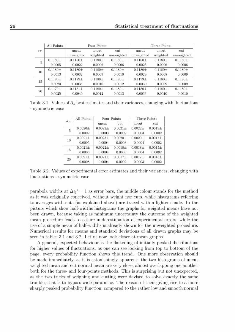
We have chosen a gaussian probability distribution function because of the rea-sons explained at the end of section 3.1. In order to make graphs and numerical re-sults look real as much as possible (this has no consequence upon method goodness),for the analysis that follows, the parabola has been chosen to have the minimum forαs = 0.118 and an half-width of 0.002, as these are approximately current results forits value [8]. The minimum value of χ2 has been set at 3415, its expected outcomefor data sets without inconsistency; note that this parameter has no effect whatso-ever upon the resulting distributions, as it does not affect positions of minima andwidths on the x-axis.
3.4 Results
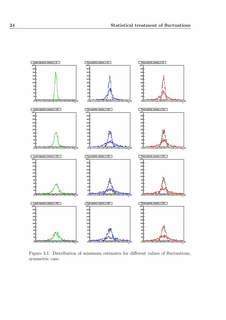
At first, a set of eleven points centered around the parabola minimum and spacedone from another as much as the parabola half-width, namely
0.108, 0.110, 0.112, 0.114, 0.116, 0.118, 0.120, 0.122, 0.124, 0.126, 0.128,
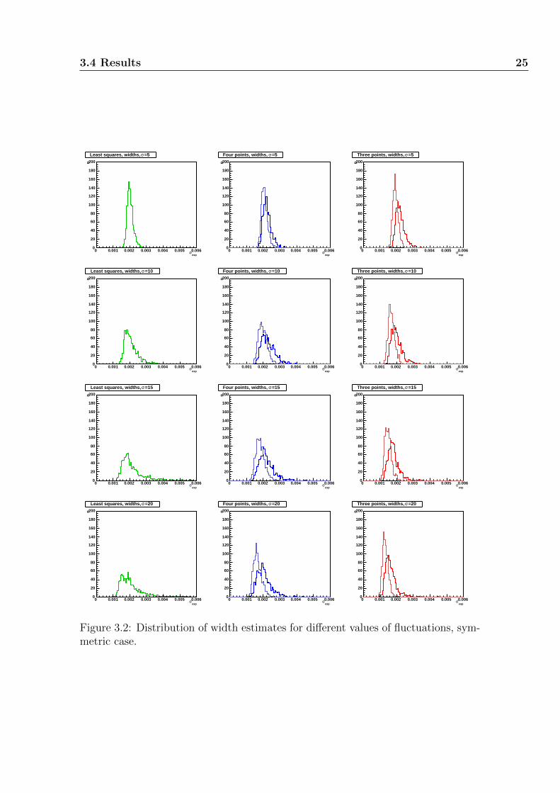
has been used. Note that these values are perfectly symmetric with respect tothe said minimum. The resulting histograms for the best estimates of the strongcoupling according to the different methods are shown in figure 3.1, while theirmatching experimental uncertainties histograms can be seen in figure 3.2. For eachhistogram a set of 1000 simulations has been used; the resulting shapes are smoothenough to guarantee that the number of toy computations is as high as is needed forresults to be stable. Each row of the graph sheets is associated to a specific varianceof the fluctuations, which takes the values 5, 10, 15 and 20 when going from pagetop to bottom; all the histograms have the same scale and could have been drawnin the same pad, though it has been decided to divide them in order to allow aneasier reading of pictures. The first column refers to results obtained through asingle parabola which interpolates points best according to the maximum likelihoodprinciple. The second and third columns are related with the four- and three-pointsmethods respectively. In each pad for the means of these two columns three graphsare drawn: the darkest represents results obtained through weighting minima with
24 Statistical treatment of fluctuations
sα 0.108 0.11 0.1120.1140.1160.118 0.12 0.1220.1240.1260.128
n
0
20
40
60
80
100
120
140
160
180
200
=5σLeast squares, means,
sα 0.108 0.11 0.1120.1140.1160.118 0.12 0.1220.1240.1260.128
n
0
20
40
60
80
100
120
140
160
180
200
=5σFour points, means,
sα 0.108 0.11 0.1120.1140.1160.118 0.12 0.1220.1240.1260.128
n
0
20
40
60
80
100
120
140
160
180
200
=5σThree points, means,
sα 0.108 0.11 0.1120.1140.1160.118 0.12 0.1220.1240.1260.128
n
0
20
40
60
80
100
120
140
160
180
200
=10σLeast squares, means,
sα 0.108 0.11 0.1120.1140.1160.118 0.12 0.1220.1240.1260.128
n
0
20
40
60
80
100
120
140
160
180
200
=10σFour points, means,
sα 0.108 0.11 0.1120.1140.1160.118 0.12 0.1220.1240.1260.128
n
0
20
40
60
80
100
120
140
160
180
200
=10σThree points, means,
sα 0.108 0.11 0.1120.1140.1160.118 0.12 0.1220.1240.1260.128
n
0
20
40
60
80
100
120
140
160
180
200
=15σLeast squares, means,
sα 0.108 0.11 0.1120.1140.1160.118 0.12 0.1220.1240.1260.128
n
0
20
40
60
80
100
120
140
160
180
200
=15σFour points, means,
sα 0.108 0.11 0.1120.1140.1160.118 0.12 0.1220.1240.1260.128
n
0
20
40
60
80
100
120
140
160
180
200
=15σThree points, means,
sα 0.108 0.11 0.1120.1140.1160.118 0.12 0.1220.1240.1260.128
n
0
20
40
60
80
100
120
140
160
180
200
=20σLeast squares, means,
sα 0.108 0.11 0.1120.1140.1160.118 0.12 0.1220.1240.1260.128
n
0
20
40
60
80
100
120
140
160
180
200
=20σFour points, means,
sα 0.108 0.11 0.1120.1140.1160.118 0.12 0.1220.1240.1260.128
n
0
20
40
60
80
100
120
140
160
180
200
=20σThree points, means,
Figure 3.1: Distribution of minimum estimates for different values of fluctuations,symmetric case.
3.4 Results 25
expσ 0 0.001 0.002 0.003 0.004 0.005 0.006
n
0
20
40
60
80
100
120
140
160
180
200
=5σLeast squares, widths,
expσ 0 0.001 0.002 0.003 0.004 0.005 0.006
n
0
20
40
60
80
100
120
140
160
180
200
=5σFour points, widths,
expσ 0 0.001 0.002 0.003 0.004 0.005 0.006
n
0
20
40
60
80
100
120
140
160
180
200
=5σThree points, widths,
expσ 0 0.001 0.002 0.003 0.004 0.005 0.006
n
0
20
40
60
80
100
120
140
160
180
200
=10σLeast squares, widths,
expσ 0 0.001 0.002 0.003 0.004 0.005 0.006
n
0
20
40
60
80
100
120
140
160
180
200
=10σFour points, widths,
expσ 0 0.001 0.002 0.003 0.004 0.005 0.006
n
0
20
40
60
80
100
120
140
160
180
200
=10σThree points, widths,
expσ 0 0.001 0.002 0.003 0.004 0.005 0.006
n
0
20
40
60
80
100
120
140
160
180
200
=15σLeast squares, widths,
expσ 0 0.001 0.002 0.003 0.004 0.005 0.006
n
0
20
40
60
80
100
120
140
160
180
200
=15σFour points, widths,
expσ 0 0.001 0.002 0.003 0.004 0.005 0.006
n
0
20
40
60
80
100
120
140
160
180
200
=15σThree points, widths,
expσ 0 0.001 0.002 0.003 0.004 0.005 0.006
n
0
20
40
60
80
100
120
140
160
180
200
=20σLeast squares, widths,
expσ 0 0.001 0.002 0.003 0.004 0.005 0.006
n
0
20
40
60
80
100
120
140
160
180
200
=20σFour points, widths,
expσ 0 0.001 0.002 0.003 0.004 0.005 0.006
n
0
20
40
60
80
100
120
140
160
180
200
=20σThree points, widths,
Figure 3.2: Distribution of width estimates for different values of fluctuations, sym-metric case.
26 Statistical treatment of fluctuations
σF
All Points Four Points Three Points
uncut uncut cut uncut uncut cut
unweighted weighted unweighted unweighted weighted unweighted
50.1180± 0.1180± 0.1180± 0.1180± 0.1180± 0.1180± 0.1180±0.0005 0.0022 0.0006 0.0006 0.0025 0.0006 0.0006
100.1180± 0.1180± 0.1180± 0.1180± 0.1180± 0.1180± 0.1180±0.0013 0.0032 0.0009 0.0010 0.0029 0.0008 0.0009
150.1180± 0.1179± 0.1180± 0.1180± 0.1179± 0.1180± 0.1180±0.0020 0.0035 0.0010 0.0012 0.0030 0.0009 0.0009
200.1179± 0.1181± 0.1180± 0.1180± 0.1180± 0.1180± 0.1180±0.0025 0.0040 0.0012 0.0013 0.0033 0.0010 0.0010
Table 3.1: Values of αs best estimates and their variances, changing with fluctuations- symmetric case
σFAll Points Four Points Three Points
uncut cut uncut cut
50.0020± 0.0022± 0.0021± 0.0022± 0.0019±0.0002 0.0003 0.0002 0.0003 0.0002
100.0021± 0.0023± 0.0020± 0.0020± 0.0017±0.0005 0.0004 0.0003 0.0004 0.0002
150.0021± 0.0022± 0.0018± 0.0018± 0.0015±0.0006 0.0004 0.0003 0.0004 0.0002
200.0021± 0.0021± 0.0017± 0.0017± 0.0013±0.0008 0.0004 0.0002 0.0003 0.0002
Table 3.2: Values of experimental error estimates and their variances, changing withfluctuations - symmetric case
parabola widths at ∆χ2 = 1 as error bars, the middle colour stands for the methodas it was originally conceived, without weight nor cuts, while histograms referringto averages with cuts (as explained above) are traced with a lighter shade. In thepicture which show half-widths histograms the graphs for weighted means have notbeen drawn, because taking as minimum uncertainty the outcome of the weightedmean procedure leads to a sure underestimation of experimental errors, while theuse of a simple mean of half-widths is already shown for the unweighted procedure.Numerical results for means and standard deviations of all drawn graphs may beseen in tables 3.1 and 3.2. Let us now look closer at mean graphs.
A general, expected behaviour is the flattening of initially peaked distributionsfor higher values of fluctuations; as one can see looking from top to bottom of thepage, every probability function shows this trend. One more observation shouldbe made immediately, as it is astonishingly apparent: the two histograms of uncutweighted mean and cut normal mean are very close, almost overlapping one anotherboth for the three- and four-points methods. This is surprising but not unexpected,as the two tricks of weighing and cutting were devised to solve exactly the sametrouble, that is to bypass wide parabolae. The reason of their giving rise to a moresharply peaked probability function, compared to the rather low and smooth normal
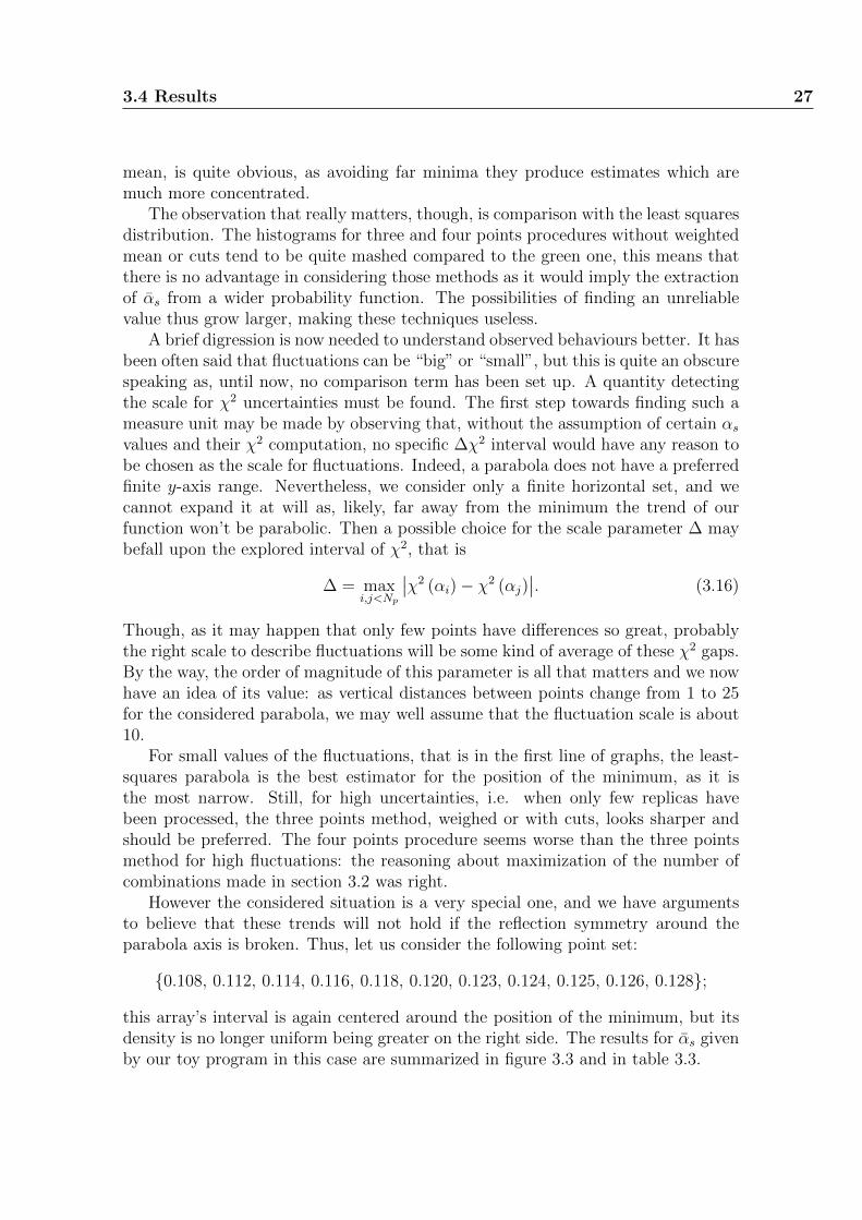
3.4 Results 27
mean, is quite obvious, as avoiding far minima they produce estimates which aremuch more concentrated.
The observation that really matters, though, is comparison with the least squaresdistribution. The histograms for three and four points procedures without weightedmean or cuts tend to be quite mashed compared to the green one, this means thatthere is no advantage in considering those methods as it would imply the extractionof αs from a wider probability function. The possibilities of finding an unreliablevalue thus grow larger, making these techniques useless.
A brief digression is now needed to understand observed behaviours better. It hasbeen often said that fluctuations can be “big” or “small”, but this is quite an obscurespeaking as, until now, no comparison term has been set up. A quantity detectingthe scale for χ2 uncertainties must be found. The first step towards finding such ameasure unit may be made by observing that, without the assumption of certain αsvalues and their χ2 computation, no specific ∆χ2 interval would have any reason tobe chosen as the scale for fluctuations. Indeed, a parabola does not have a preferredfinite y-axis range. Nevertheless, we consider only a finite horizontal set, and wecannot expand it at will as, likely, far away from the minimum the trend of ourfunction won’t be parabolic. Then a possible choice for the scale parameter ∆ maybefall upon the explored interval of χ2, that is
∆ = maxi,j<Np
∣∣χ2 (αi)− χ2 (αj)∣∣. (3.16)
Though, as it may happen that only few points have differences so great, probablythe right scale to describe fluctuations will be some kind of average of these χ2 gaps.By the way, the order of magnitude of this parameter is all that matters and we nowhave an idea of its value: as vertical distances between points change from 1 to 25for the considered parabola, we may well assume that the fluctuation scale is about10.
For small values of the fluctuations, that is in the first line of graphs, the least-squares parabola is the best estimator for the position of the minimum, as it isthe most narrow. Still, for high uncertainties, i.e. when only few replicas havebeen processed, the three points method, weighed or with cuts, looks sharper andshould be preferred. The four points procedure seems worse than the three pointsmethod for high fluctuations: the reasoning about maximization of the number ofcombinations made in section 3.2 was right.
However the considered situation is a very special one, and we have argumentsto believe that these trends will not hold if the reflection symmetry around theparabola axis is broken. Thus, let us consider the following point set:
0.108, 0.112, 0.114, 0.116, 0.118, 0.120, 0.123, 0.124, 0.125, 0.126, 0.128;
this array’s interval is again centered around the position of the minimum, but itsdensity is no longer uniform being greater on the right side. The results for αs givenby our toy program in this case are summarized in figure 3.3 and in table 3.3.
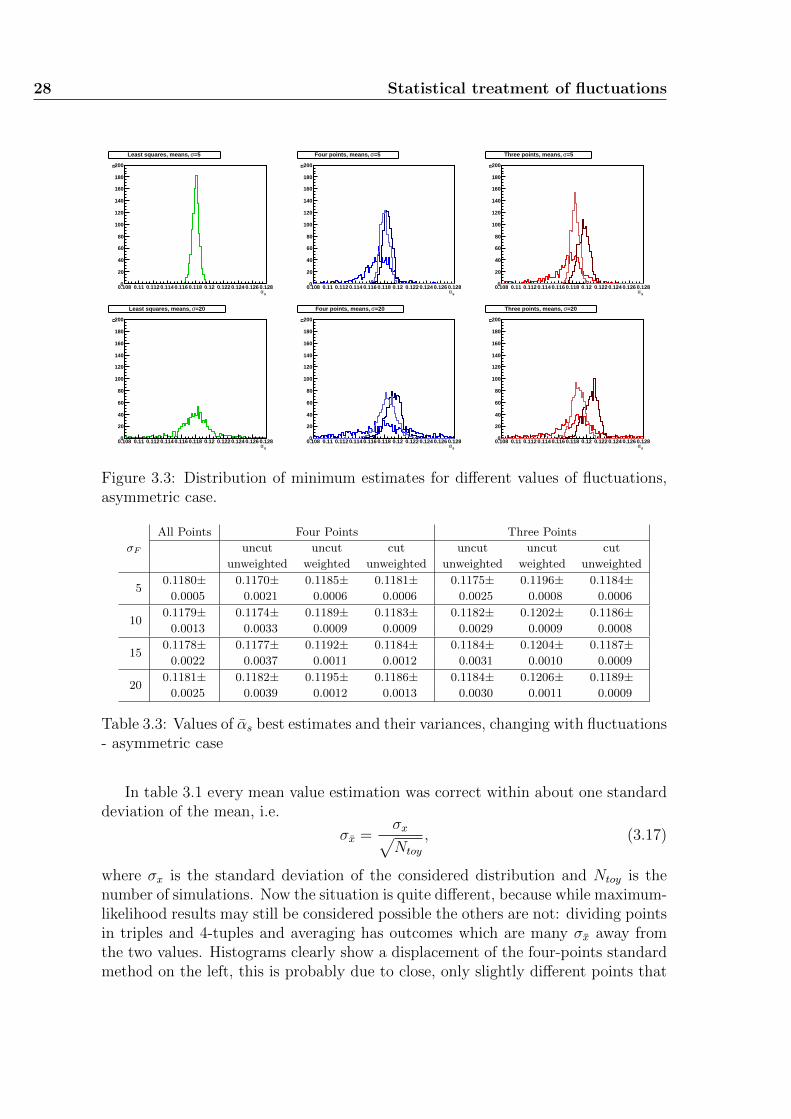
28 Statistical treatment of fluctuations
sα 0.108 0.11 0.112 0.114 0.116 0.118 0.12 0.122 0.124 0.126 0.128
n
0
20
40
60
80
100
120
140
160
180
200
=5σLeast squares, means,
sα 0.108 0.11 0.112 0.114 0.116 0.118 0.12 0.122 0.124 0.126 0.128
n
0
20
40
60
80
100
120
140
160
180
200
=5σFour points, means,
sα 0.108 0.11 0.112 0.114 0.116 0.118 0.12 0.122 0.124 0.126 0.128
n
0
20
40
60
80
100
120
140
160
180
200
=5σThree points, means,
sα 0.108 0.11 0.112 0.114 0.116 0.118 0.12 0.122 0.124 0.126 0.128
n
0
20
40
60
80
100
120
140
160
180
200
=20σLeast squares, means,
sα 0.108 0.11 0.112 0.114 0.116 0.118 0.12 0.122 0.124 0.126 0.128
n
0
20
40
60
80
100
120
140
160
180
200
=20σFour points, means,
sα 0.108 0.11 0.112 0.114 0.116 0.118 0.12 0.122 0.124 0.126 0.128
n
0
20
40
60
80
100
120
140
160
180
200
=20σThree points, means,
Figure 3.3: Distribution of minimum estimates for different values of fluctuations,asymmetric case.
σF
All Points Four Points Three Points
uncut uncut cut uncut uncut cut
unweighted weighted unweighted unweighted weighted unweighted
50.1180± 0.1170± 0.1185± 0.1181± 0.1175± 0.1196± 0.1184±0.0005 0.0021 0.0006 0.0006 0.0025 0.0008 0.0006
100.1179± 0.1174± 0.1189± 0.1183± 0.1182± 0.1202± 0.1186±0.0013 0.0033 0.0009 0.0009 0.0029 0.0009 0.0008
150.1178± 0.1177± 0.1192± 0.1184± 0.1184± 0.1204± 0.1187±0.0022 0.0037 0.0011 0.0012 0.0031 0.0010 0.0009
200.1181± 0.1182± 0.1195± 0.1186± 0.1184± 0.1206± 0.1189±0.0025 0.0039 0.0012 0.0013 0.0030 0.0011 0.0009
Table 3.3: Values of αs best estimates and their variances, changing with fluctuations- asymmetric case
In table 3.1 every mean value estimation was correct within about one standarddeviation of the mean, i.e.
σx =σx√Ntoy
, (3.17)
where σx is the standard deviation of the considered distribution and Ntoy is thenumber of simulations. Now the situation is quite different, because while maximum-likelihood results may still be considered possible the others are not: dividing pointsin triples and 4-tuples and averaging has outcomes which are many σx away fromthe two values. Histograms clearly show a displacement of the four-points standardmethod on the left, this is probably due to close, only slightly different points that
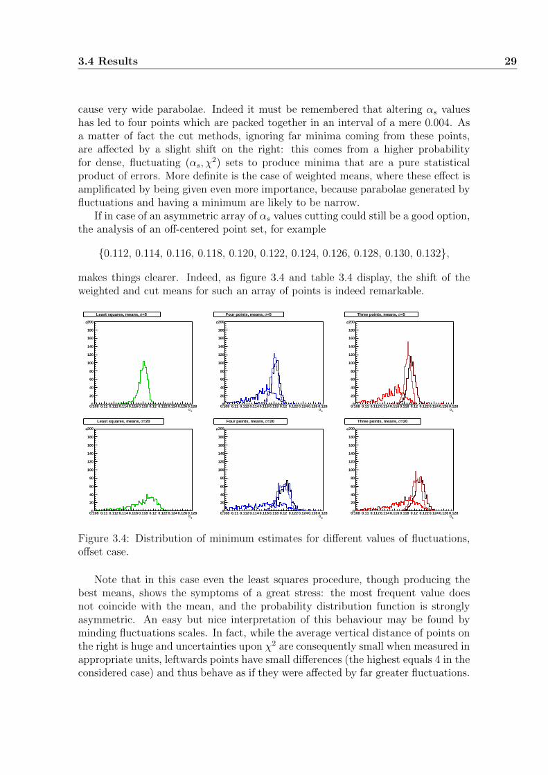
3.4 Results 29
cause very wide parabolae. Indeed it must be remembered that altering αs valueshas led to four points which are packed together in an interval of a mere 0.004. Asa matter of fact the cut methods, ignoring far minima coming from these points,are affected by a slight shift on the right: this comes from a higher probabilityfor dense, fluctuating (αs, χ
2) sets to produce minima that are a pure statisticalproduct of errors. More definite is the case of weighted means, where these effect isamplificated by being given even more importance, because parabolae generated byfluctuations and having a minimum are likely to be narrow.
If in case of an asymmetric array of αs values cutting could still be a good option,the analysis of an off-centered point set, for example
0.112, 0.114, 0.116, 0.118, 0.120, 0.122, 0.124, 0.126, 0.128, 0.130, 0.132,
makes things clearer. Indeed, as figure 3.4 and table 3.4 display, the shift of theweighted and cut means for such an array of points is indeed remarkable.
sα 0.108 0.11 0.112 0.114 0.116 0.118 0.12 0.122 0.124 0.126 0.128
n
0
20
40
60
80
100
120
140
160
180
200
=5σLeast squares, means,
sα 0.108 0.11 0.112 0.114 0.116 0.118 0.12 0.122 0.124 0.126 0.128
n
0
20
40
60
80
100
120
140
160
180
200
=5σFour points, means,
sα 0.108 0.11 0.112 0.114 0.116 0.118 0.12 0.122 0.124 0.126 0.128
n
0
20
40
60
80
100
120
140
160
180
200
=5σThree points, means,
sα 0.108 0.11 0.112 0.114 0.116 0.118 0.12 0.122 0.124 0.126 0.128
n
0
20
40
60
80
100
120
140
160
180
200
=20σLeast squares, means,
sα 0.108 0.11 0.112 0.114 0.116 0.118 0.12 0.122 0.124 0.126 0.128
n
0
20
40
60
80
100
120
140
160
180
200
=20σFour points, means,
sα 0.108 0.11 0.112 0.114 0.116 0.118 0.12 0.122 0.124 0.126 0.128
n
0
20
40
60
80
100
120
140
160
180
200
=20σThree points, means,
Figure 3.4: Distribution of minimum estimates for different values of fluctuations,offset case.
Note that in this case even the least squares procedure, though producing thebest means, shows the symptoms of a great stress: the most frequent value doesnot coincide with the mean, and the probability distribution function is stronglyasymmetric. An easy but nice interpretation of this behaviour may be found byminding fluctuations scales. In fact, while the average vertical distance of points onthe right is huge and uncertainties upon χ2 are consequently small when measured inappropriate units, leftwards points have small differences (the highest equals 4 in theconsidered case) and thus behave as if they were affected by far greater fluctuations.
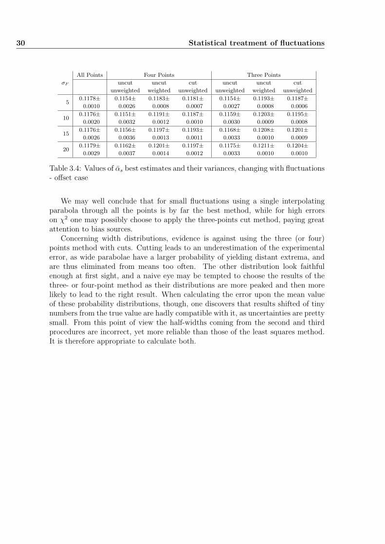
30 Statistical treatment of fluctuations
σF
All Points Four Points Three Points
uncut uncut cut uncut uncut cut
unweighted weighted unweighted unweighted weighted unweighted
50.1178± 0.1154± 0.1183± 0.1181± 0.1154± 0.1193± 0.1187±0.0010 0.0026 0.0008 0.0007 0.0027 0.0008 0.0006
100.1176± 0.1151± 0.1191± 0.1187± 0.1159± 0.1203± 0.1195±0.0020 0.0032 0.0012 0.0010 0.0030 0.0009 0.0008
150.1176± 0.1156± 0.1197± 0.1193± 0.1168± 0.1208± 0.1201±0.0026 0.0036 0.0013 0.0011 0.0033 0.0010 0.0009
200.1179± 0.1162± 0.1201± 0.1197± 0.1175± 0.1211± 0.1204±0.0029 0.0037 0.0014 0.0012 0.0033 0.0010 0.0010
Table 3.4: Values of αs best estimates and their variances, changing with fluctuations- offset case
We may well conclude that for small fluctuations using a single interpolatingparabola through all the points is by far the best method, while for high errorson χ2 one may possibly choose to apply the three-points cut method, paying greatattention to bias sources.
Concerning width distributions, evidence is against using the three (or four)points method with cuts. Cutting leads to an underestimation of the experimentalerror, as wide parabolae have a larger probability of yielding distant extrema, andare thus eliminated from means too often. The other distribution look faithfulenough at first sight, and a naive eye may be tempted to choose the results of thethree- or four-point method as their distributions are more peaked and then morelikely to lead to the right result. When calculating the error upon the mean valueof these probability distributions, though, one discovers that results shifted of tinynumbers from the true value are hadly compatible with it, as uncertainties are prettysmall. From this point of view the half-widths coming from the second and thirdprocedures are incorrect, yet more reliable than those of the least squares method.It is therefore appropriate to calculate both.
Chapter 4
Determination of the strongcoupling constant
4.1 A new look on NNPDF 1.2 data
The first data set we will look into, now we have chosen our procedures, is the oneanalyzed in reference [7]. These values of χ2(αs), summarized in table 4.1, havebeen obtained using version 1.2 of NNPDF, which includes as a source only deepinelastic scattering experiments.
Due to the discovery of a bug in the program which was used to study theseresults in the cited work, it is indeed worth to look at them again. Moreover, thesedata shall be a good ground for testing the discussed techniques, their strengths andtheir weaknesses.
Let us first consider the results obtained applying blindly to all total χ2 pointsthe maximum-likelihood method and the three-points cut procedure; the parabolaewhich are the graphical representation of means and experimental errors are drawnin figure 4.1, while numerical results are:
Parabola through all the points: αs = 0.1202± 0.0004(exp); (4.1)
Three points cut parabola: αs = 0.1219± 0.0005(exp). (4.2)
These outcomes do not agree with each other, and the reason for such a discrep-ancy is hinted by the graphs. Indeed it must be remembered that (αs, χ
2) pointsresulting from NNPDF computation are not located on a parabolic curve for everyhorizontal interval: in this case, this may be seen by looking at the green line whichshould interpolate all the points, while as a matter of fact it is far too narrow tofit the left-central region and yet not bent enough to pass through rightwards data.Instead the effect on the red curve coming from these two right points, associatedto αs = 0.135 and 0.140, is only a vertical shift: one could imagine to lower thisparabola and discover that it fits the central region very well.
Another suggestion to solve the problem is the strong asymmetry of points.While for high values of αs the graph rises steadily, it does not go up with the
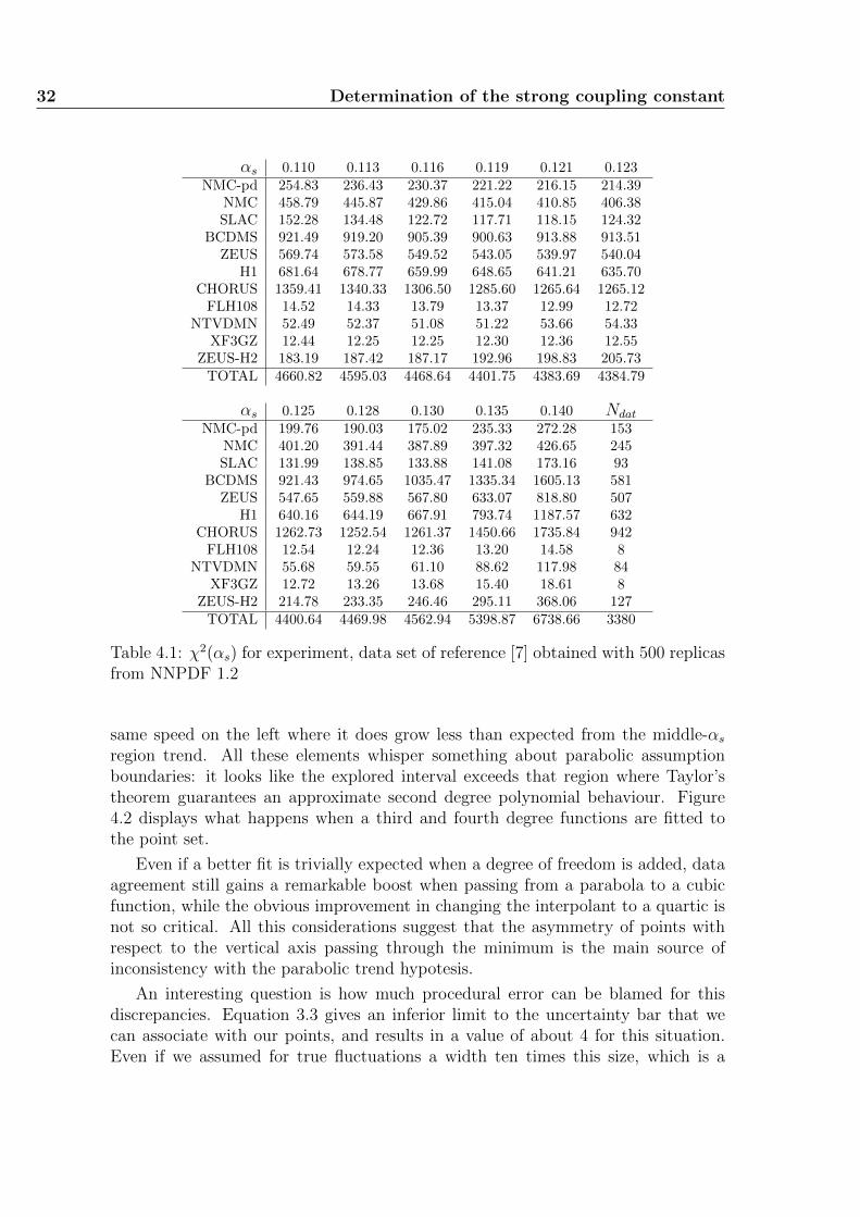
32 Determination of the strong coupling constant
αs 0.110 0.113 0.116 0.119 0.121 0.123NMC-pd 254.83 236.43 230.37 221.22 216.15 214.39
NMC 458.79 445.87 429.86 415.04 410.85 406.38SLAC 152.28 134.48 122.72 117.71 118.15 124.32
BCDMS 921.49 919.20 905.39 900.63 913.88 913.51ZEUS 569.74 573.58 549.52 543.05 539.97 540.04
H1 681.64 678.77 659.99 648.65 641.21 635.70CHORUS 1359.41 1340.33 1306.50 1285.60 1265.64 1265.12
FLH108 14.52 14.33 13.79 13.37 12.99 12.72NTVDMN 52.49 52.37 51.08 51.22 53.66 54.33
XF3GZ 12.44 12.25 12.25 12.30 12.36 12.55ZEUS-H2 183.19 187.42 187.17 192.96 198.83 205.73
TOTAL 4660.82 4595.03 4468.64 4401.75 4383.69 4384.79
αs 0.125 0.128 0.130 0.135 0.140 Ndat
NMC-pd 199.76 190.03 175.02 235.33 272.28 153NMC 401.20 391.44 387.89 397.32 426.65 245SLAC 131.99 138.85 133.88 141.08 173.16 93
BCDMS 921.43 974.65 1035.47 1335.34 1605.13 581ZEUS 547.65 559.88 567.80 633.07 818.80 507
H1 640.16 644.19 667.91 793.74 1187.57 632CHORUS 1262.73 1252.54 1261.37 1450.66 1735.84 942
FLH108 12.54 12.24 12.36 13.20 14.58 8NTVDMN 55.68 59.55 61.10 88.62 117.98 84
XF3GZ 12.72 13.26 13.68 15.40 18.61 8ZEUS-H2 214.78 233.35 246.46 295.11 368.06 127
TOTAL 4400.64 4469.98 4562.94 5398.87 6738.66 3380
Table 4.1: χ2(αs) for experiment, data set of reference [7] obtained with 500 replicasfrom NNPDF 1.2
same speed on the left where it does grow less than expected from the middle-αsregion trend. All these elements whisper something about parabolic assumptionboundaries: it looks like the explored interval exceeds that region where Taylor’stheorem guarantees an approximate second degree polynomial behaviour. Figure4.2 displays what happens when a third and fourth degree functions are fitted tothe point set.
Even if a better fit is trivially expected when a degree of freedom is added, dataagreement still gains a remarkable boost when passing from a parabola to a cubicfunction, while the obvious improvement in changing the interpolant to a quartic isnot so critical. All this considerations suggest that the asymmetry of points withrespect to the vertical axis passing through the minimum is the main source ofinconsistency with the parabolic trend hypotesis.
An interesting question is how much procedural error can be blamed for thisdiscrepancies. Equation 3.3 gives an inferior limit to the uncertainty bar that wecan associate with our points, and results in a value of about 4 for this situation.Even if we assumed for true fluctuations a width ten times this size, which is a

4.1 A new look on NNPDF 1.2 data 33
sα 0.11 0.115 0.12 0.125 0.13 0.135 0.14
2 χ
4500
5000
5500
6000
6500
2χTotal
Figure 4.1: Graphical representation of results for the NNPDF1.2 data set.Green stands for least squares parabola, while in red results of the three points cutmethod are drawn.
sα 0.11 0.115 0.12 0.125 0.13 0.135 0.14
2 χ
4500
5000
5500
6000
6500
Quadratic function
sα 0.11 0.115 0.12 0.125 0.13 0.135 0.14
2 χ
4500
5000
5500
6000
6500
Cubic function
sα 0.11 0.115 0.12 0.125 0.13 0.135 0.14
2 χ
4500
5000
5500
6000
6500
Quartic function
Figure 4.2: NNPDF1.2 data set fit with a second, third and fourth degree polyno-mials.
good deal larger than expected, still errors would be very small when drawn on thegraph and would not quantitatively explain the general disagreement that appearsqualitatively evident. Thus the badness of fit cannot be an effect of fluctuations andthe validity of the parabolic approximation on the whole interval has been rejectedby experimental evidence.
A reasonable choice to restore the conditions needed to apply our techniques isto neglect points which are further away from the minimum than, say, 20σexp; asthe three points method is supposed to be more similar to the next result, its valuesfor the mean and the half-width are assumed to perform this operation. Then the xaxis values not to be kept are those falling outside [0.1119, 0.1319], namely one on
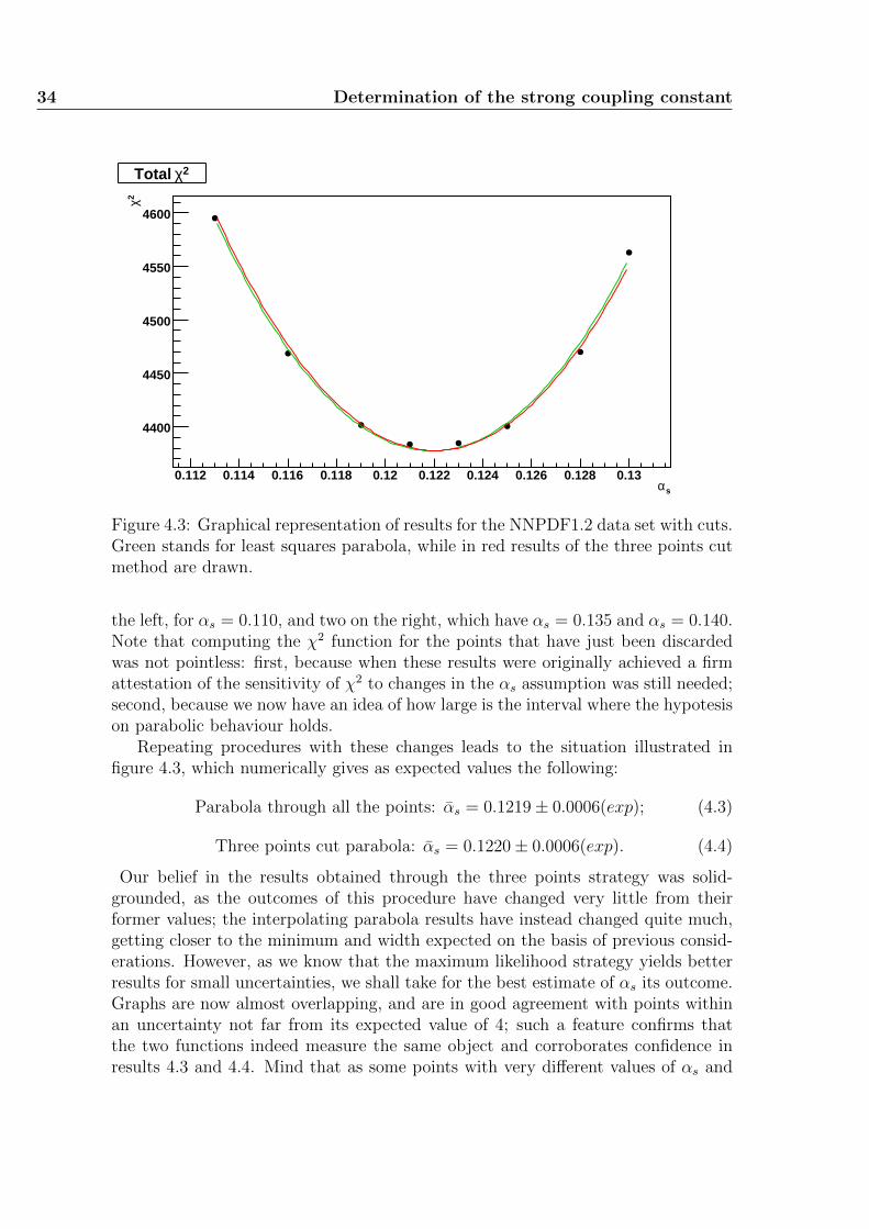
34 Determination of the strong coupling constant
sα 0.112 0.114 0.116 0.118 0.12 0.122 0.124 0.126 0.128 0.13
2 χ
4400
4450
4500
4550
4600
2χTotal
Figure 4.3: Graphical representation of results for the NNPDF1.2 data set with cuts.Green stands for least squares parabola, while in red results of the three points cutmethod are drawn.
the left, for αs = 0.110, and two on the right, which have αs = 0.135 and αs = 0.140.Note that computing the χ2 function for the points that have just been discardedwas not pointless: first, because when these results were originally achieved a firmattestation of the sensitivity of χ2 to changes in the αs assumption was still needed;second, because we now have an idea of how large is the interval where the hypotesison parabolic behaviour holds.
Repeating procedures with these changes leads to the situation illustrated infigure 4.3, which numerically gives as expected values the following:
Parabola through all the points: αs = 0.1219± 0.0006(exp); (4.3)
Three points cut parabola: αs = 0.1220± 0.0006(exp). (4.4)
Our belief in the results obtained through the three points strategy was solid-grounded, as the outcomes of this procedure have changed very little from theirformer values; the interpolating parabola results have instead changed quite much,getting closer to the minimum and width expected on the basis of previous consid-erations. However, as we know that the maximum likelihood strategy yields betterresults for small uncertainties, we shall take for the best estimate of αs its outcome.Graphs are now almost overlapping, and are in good agreement with points withinan uncertainty not far from its expected value of 4; such a feature confirms thatthe two functions indeed measure the same object and corroborates confidence inresults 4.3 and 4.4. Mind that as some points with very different values of αs and
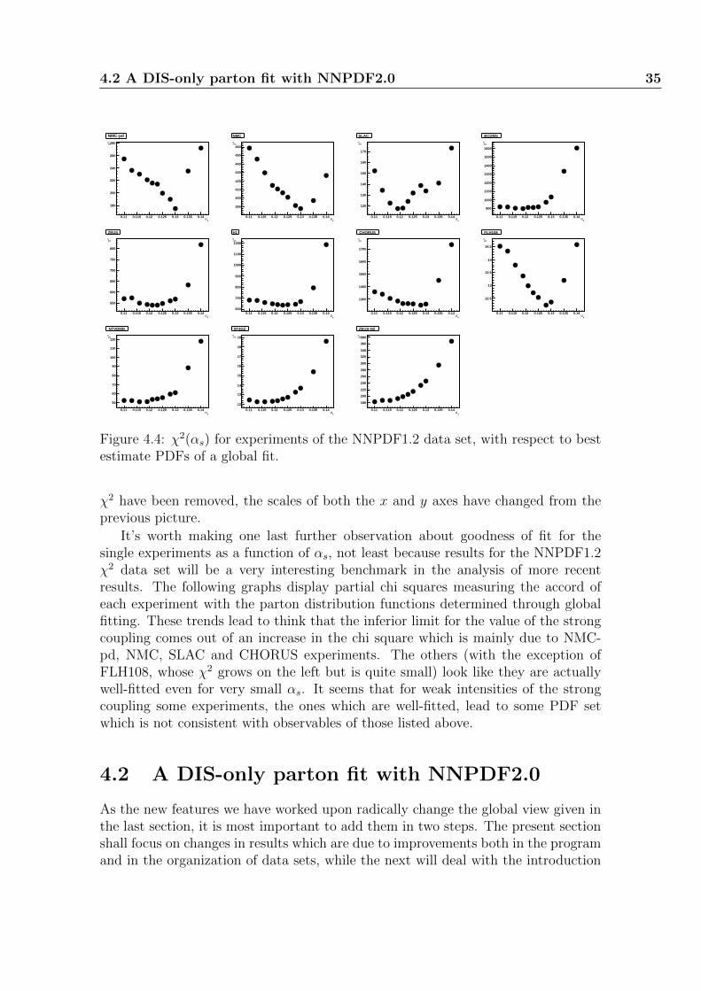
4.2 A DIS-only parton fit with NNPDF2.0 35
sα 0.11 0.115 0.12 0.125 0.13 0.135 0.14
2 χ
180
200
220
240
260
280
NMC-pd
sα 0.11 0.115 0.12 0.125 0.13 0.135 0.14
2 χ
390
400
410
420
430
440
450
460
NMC
sα 0.11 0.115 0.12 0.125 0.13 0.135 0.14
2 χ
120
130
140
150
160
170
SLAC
sα 0.11 0.115 0.12 0.125 0.13 0.135 0.14
2 χ
900
1000
1100
1200
1300
1400
1500
1600
BCDMS
sα
0.11 0.115 0.12 0.125 0.13 0.135 0.14
2 χ
550
600
650
700
750
800
ZEUS
sα
0.11 0.115 0.12 0.125 0.13 0.135 0.14
2 χ
600
700
800
900
1000
1100
1200
H1
sα
0.11 0.115 0.12 0.125 0.13 0.135 0.14
2 χ
1300
1400
1500
1600
1700
CHORUS
sα
0.11 0.115 0.12 0.125 0.13 0.135 0.14
2 χ
12.5
13
13.5
14
14.5
FLH108
sα
0.11 0.115 0.12 0.125 0.13 0.135 0.14
2 χ
50
60
70
80
90
100
110
120
NTVDMN
sα
0.11 0.115 0.12 0.125 0.13 0.135 0.14
2 χ
12
13
14
15
16
17
18
19
XF3GZ
sα
0.11 0.115 0.12 0.125 0.13 0.135 0.14
2 χ
180
200
220
240
260
280
300
320
340
360
380
ZEUS-H2
Figure 4.4: χ2(αs) for experiments of the NNPDF1.2 data set, with respect to bestestimate PDFs of a global fit.
χ2 have been removed, the scales of both the x and y axes have changed from theprevious picture.
It’s worth making one last further observation about goodness of fit for thesingle experiments as a function of αs, not least because results for the NNPDF1.2χ2 data set will be a very interesting benchmark in the analysis of more recentresults. The following graphs display partial chi squares measuring the accord ofeach experiment with the parton distribution functions determined through globalfitting. These trends lead to think that the inferior limit for the value of the strongcoupling comes out of an increase in the chi square which is mainly due to NMC-pd, NMC, SLAC and CHORUS experiments. The others (with the exception ofFLH108, whose χ2 grows on the left but is quite small) look like they are actuallywell-fitted even for very small αs. It seems that for weak intensities of the strongcoupling some experiments, the ones which are well-fitted, lead to some PDF setwhich is not consistent with observables of those listed above.
4.2 A DIS-only parton fit with NNPDF2.0
As the new features we have worked upon radically change the global view given inthe last section, it is most important to add them in two steps. The present sectionshall focus on changes in results which are due to improvements both in the programand in the organization of data sets, while the next will deal with the introduction
36 Determination of the strong coupling constant
of Drell-Yan and hadronic jet experiments as new sources of information to allowa better extraction of parton distribution functions. The main differences between1.2 and 2.0 data are traced in section 2.2; here we concentrate upon finding the bestvalue of αs for the considered ensemble.
The original idea was to use a set of seven values for αs, approximately centeredon the value that is usually assumed for it and spaced as much as its uncertainty,namely 0.112, 0.114, 0.116, 0.118, 0.120, 0.122, 0.124. Note that selecting closer val-ues would mean to handle smaller χ2 differences which require a higher numberof replicas to carry reliable information. Moreover it must be remembered that,while the machine-time required to perform parton fits grows linearly with Nrep, theorder of magnitude of random fluctuations around the correct χ2 value gets loweronly as 1/
√Nrep. Thus, globally, increasing the points’ accuracy needs a time that
increases asymptotically as the square root of accuracy itself. One could be thentempted to work with many, highly fluctuating points for very close values of αs,but here two complications arise. First, this choice would mean dealing with hardlyinconsistent data, and saying goodbye to the possibility of seeing reasonable, easilyinterpreted graphs. The second and more immediately compelling trouble is thatfor every value of the strong coupling different evolution kernels must be computed,and this requires running another program. A constant time must then be addedto the length of training for Nrep PDF sets, if one wants to obtain the actual timeneeded to have Nrep replicas for a given point.
This is why we thought evaluating χ2 (αs) for about ten points was a reasonabledecision. Then we started with the values above, plus the extra point αs = 0.119whose evolution tables were already available. However, when the stage of thefirst 100 replicas was completed, it was difficoult to exclude the possibility of theminimum being outside the chosen interval. The fluctuations were indeed still veryhigh. Thus it was decided to add two more points, at 0.105 and 0.130, that couldwork as boudaries.
Furthermore, while proceeding with the analysis, it became clear that the pre-diction for αs was much smaller than expected at the beginning. Such a small valuedemanded for more points on the left side of our initial array, and we added onemore point to extend the first set on the left as naturally as possible. We addedreplicas to those points until we reached the number of 500 for each (αs, χ
2) pairand results looked stable enough. It’s important to point out that, while our finalresults are approximately the same whichever procedure is chosen for the analysisas uncertainties due to fluctuations are rather small, in early stages the possibilityof obtaining faithful estimations for the minimum abscissa has had a great influenceon our choices. This is why so much attention was given to this problem in theprevious chapter.
Coming back to the outcomes of the parton fit, the final numerical values of χ2
are summarized in table 4.2.
The graph displaying the total chi square as a function of the strong coupling isshown in figure 4.5, and the best estimates for the extremum position and parabola
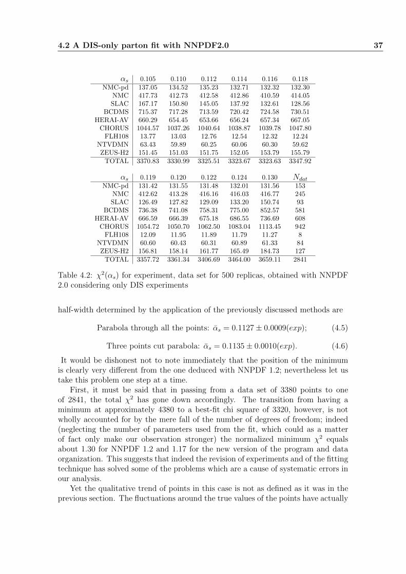
4.2 A DIS-only parton fit with NNPDF2.0 37
αs 0.105 0.110 0.112 0.114 0.116 0.118NMC-pd 137.05 134.52 135.23 132.71 132.32 132.30
NMC 417.73 412.73 412.58 412.86 410.59 414.05SLAC 167.17 150.80 145.05 137.92 132.61 128.56
BCDMS 715.37 717.28 713.59 720.42 724.58 730.51HERAI-AV 660.29 654.45 653.66 656.24 657.34 667.05
CHORUS 1044.57 1037.26 1040.64 1038.87 1039.78 1047.80FLH108 13.77 13.03 12.76 12.54 12.32 12.24
NTVDMN 63.43 59.89 60.25 60.06 60.30 59.62ZEUS-H2 151.45 151.03 151.75 152.05 153.79 155.79
TOTAL 3370.83 3330.99 3325.51 3323.67 3323.63 3347.92
αs 0.119 0.120 0.122 0.124 0.130 Ndat
NMC-pd 131.42 131.55 131.48 132.01 131.56 153NMC 412.62 413.28 416.16 416.03 416.77 245SLAC 126.49 127.82 129.09 133.20 150.74 93
BCDMS 736.38 741.08 758.31 775.00 852.57 581HERAI-AV 666.59 666.39 675.18 686.55 736.69 608
CHORUS 1054.72 1050.70 1062.50 1083.04 1113.45 942FLH108 12.09 11.95 11.89 11.79 11.27 8
NTVDMN 60.60 60.43 60.31 60.89 61.33 84ZEUS-H2 156.81 158.14 161.77 165.49 184.73 127
TOTAL 3357.72 3361.34 3406.69 3464.00 3659.11 2841
Table 4.2: χ2(αs) for experiment, data set for 500 replicas, obtained with NNPDF2.0 considering only DIS experiments
half-width determined by the application of the previously discussed methods are
Parabola through all the points: αs = 0.1127± 0.0009(exp); (4.5)
Three points cut parabola: αs = 0.1135± 0.0010(exp). (4.6)
It would be dishonest not to note immediately that the position of the minimumis clearly very different from the one deduced with NNPDF 1.2; nevertheless let ustake this problem one step at a time.
First, it must be said that in passing from a data set of 3380 points to oneof 2841, the total χ2 has gone down accordingly. The transition from having aminimum at approximately 4380 to a best-fit chi square of 3320, however, is notwholly accounted for by the mere fall of the number of degrees of freedom; indeed(neglecting the number of parameters used from the fit, which could as a matterof fact only make our observation stronger) the normalized minimum χ2 equalsabout 1.30 for NNPDF 1.2 and 1.17 for the new version of the program and dataorganization. This suggests that indeed the revision of experiments and of the fittingtechnique has solved some of the problems which are a cause of systematic errors inour analysis.
Yet the qualitative trend of points in this case is not as defined as it was in theprevious section. The fluctuations around the true values of the points have actually
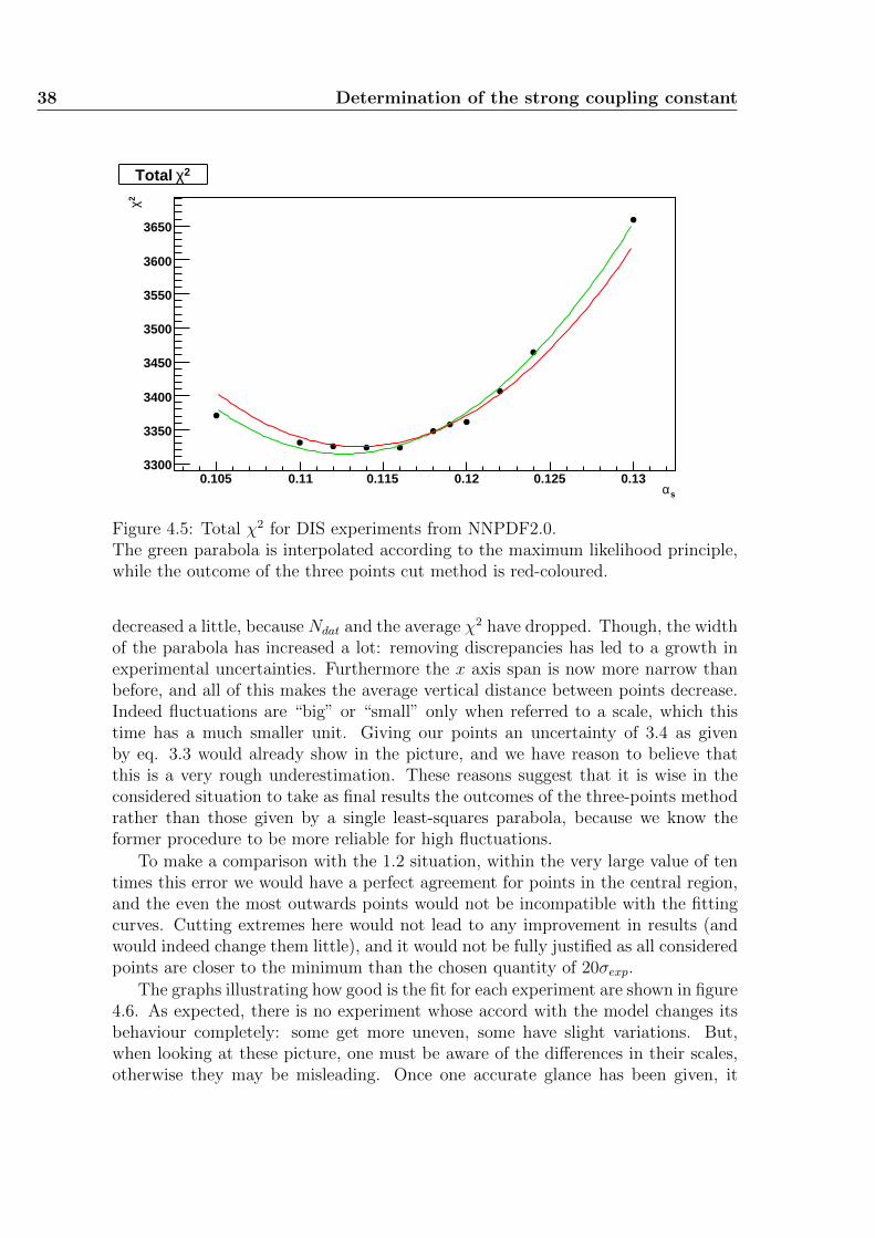
38 Determination of the strong coupling constant
sα 0.105 0.11 0.115 0.12 0.125 0.13
2 χ
3300
3350
3400
3450
3500
3550
3600
3650
2χTotal
Figure 4.5: Total χ2 for DIS experiments from NNPDF2.0.The green parabola is interpolated according to the maximum likelihood principle,while the outcome of the three points cut method is red-coloured.
decreased a little, because Ndat and the average χ2 have dropped. Though, the widthof the parabola has increased a lot: removing discrepancies has led to a growth inexperimental uncertainties. Furthermore the x axis span is now more narrow thanbefore, and all of this makes the average vertical distance between points decrease.Indeed fluctuations are “big” or “small” only when referred to a scale, which thistime has a much smaller unit. Giving our points an uncertainty of 3.4 as givenby eq. 3.3 would already show in the picture, and we have reason to believe thatthis is a very rough underestimation. These reasons suggest that it is wise in theconsidered situation to take as final results the outcomes of the three-points methodrather than those given by a single least-squares parabola, because we know theformer procedure to be more reliable for high fluctuations.
To make a comparison with the 1.2 situation, within the very large value of tentimes this error we would have a perfect agreement for points in the central region,and the even the most outwards points would not be incompatible with the fittingcurves. Cutting extremes here would not lead to any improvement in results (andwould indeed change them little), and it would not be fully justified as all consideredpoints are closer to the minimum than the chosen quantity of 20σexp.
The graphs illustrating how good is the fit for each experiment are shown in figure4.6. As expected, there is no experiment whose accord with the model changes itsbehaviour completely: some get more uneven, some have slight variations. But,when looking at these picture, one must be aware of the differences in their scales,otherwise they may be misleading. Once one accurate glance has been given, it
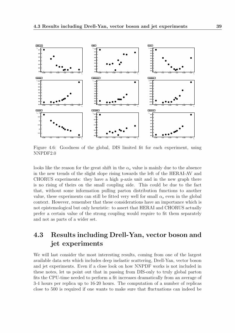
4.3 Results including Drell-Yan, vector boson and jet experiments 39
sα 0.105 0.11 0.115 0.12 0.125 0.13
2 χ
131
132
133
134
135
136
137
NMC-pd
sα 0.105 0.11 0.115 0.12 0.125 0.13
2 χ
410
411
412
413
414
415
416
417
418
NMC
sα 0.105 0.11 0.115 0.12 0.125 0.13
2 χ
125
130
135
140
145
150
155
160
165
170
SLAC
sα
0.105 0.11 0.115 0.12 0.125 0.13
2 χ
700
720
740
760
780
800
820
840
860
BCDMS
sα
0.105 0.11 0.115 0.12 0.125 0.13
2 χ
650
660
670
680
690
700
710
720
730
740
HERAI-AV
sα
0.105 0.11 0.115 0.12 0.125 0.13
2 χ
1030
1040
1050
1060
1070
1080
1090
1100
1110
1120
CHORUS
sα
0.105 0.11 0.115 0.12 0.125 0.13
2 χ
11.5
12
12.5
13
13.5
14
FLH108
sα
0.105 0.11 0.115 0.12 0.125 0.13
2 χ
59.5
60
60.5
61
61.5
62
62.5
63
63.5
NTVDMN
sα
0.105 0.11 0.115 0.12 0.125 0.13
2 χ
150
155
160
165
170
175
180
185
ZEUS-H2
Figure 4.6: Goodness of the global, DIS limited fit for each experiment, usingNNPDF2.0
looks like the reason for the great shift in the αs value is mainly due to the absencein the new trends of the slight slope rising towards the left of the HERAI-AV andCHORUS experiments: they have a high y-axis unit and in the new graph thereis no rising of theirs on the small coupling side. This could be due to the factthat, without some information pulling parton distribution functions to anothervalue, these experiments can still be fitted very well for small αs even in the globalcontext. However, remember that these considerations have an importance which isnot epistemological but only heuristic: to assert that HERAI and CHORUS actuallyprefer a certain value of the strong coupling would require to fit them separatelyand not as parts of a wider set.
4.3 Results including Drell-Yan, vector boson and
jet experiments
We will last consider the most interesting results, coming from one of the largestavailable data sets which includes deep inelastic scattering, Drell-Yan, vector bosonand jet experiments. Even if a close look on how NNPDF works is not included inthese notes, let us point out that in passing from DIS-only to truly global partonfits the CPU-time needed to perform a fit increases dramatically from an average of3-4 hours per replica up to 16-20 hours. The computation of a number of replicasclose to 500 is required if one wants to make sure that fluctuations can indeed be
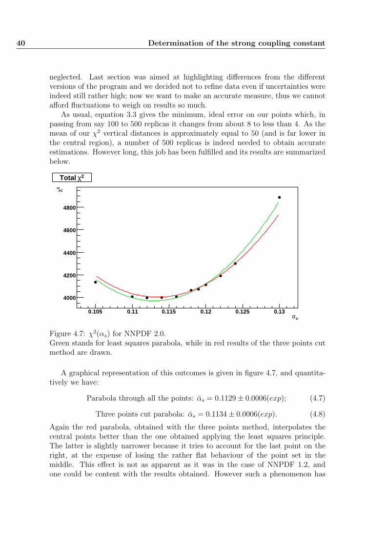
40 Determination of the strong coupling constant
neglected. Last section was aimed at highlighting differences from the differentversions of the program and we decided not to refine data even if uncertainties wereindeed still rather high; now we want to make an accurate measure, thus we cannotafford fluctuations to weigh on results so much.
As usual, equation 3.3 gives the minimum, ideal error on our points which, inpassing from say 100 to 500 replicas it changes from about 8 to less than 4. As themean of our χ2 vertical distances is approximately equal to 50 (and is far lower inthe central region), a number of 500 replicas is indeed needed to obtain accurateestimations. However long, this job has been fulfilled and its results are summarizedbelow.
sα 0.105 0.11 0.115 0.12 0.125 0.13
2 χ
4000
4200
4400
4600
4800
2χTotal
Figure 4.7: χ2(αs) for NNPDF 2.0.Green stands for least squares parabola, while in red results of the three points cutmethod are drawn.
A graphical representation of this outcomes is given in figure 4.7, and quantita-tively we have:
Parabola through all the points: αs = 0.1129± 0.0006(exp); (4.7)
Three points cut parabola: αs = 0.1134± 0.0006(exp). (4.8)
Again the red parabola, obtained with the three points method, interpolates thecentral points better than the one obtained applying the least squares principle.The latter is slightly narrower because it tries to account for the last point on theright, at the expense of losing the rather flat behaviour of the point set in themiddle. This effect is not as apparent as it was in the case of NNPDF 1.2, andone could be content with the results obtained. However such a phenomenon has
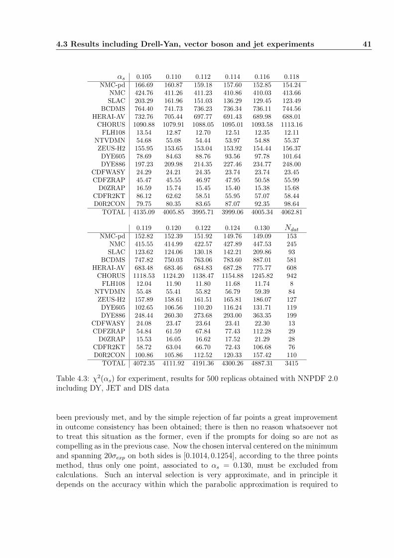
4.3 Results including Drell-Yan, vector boson and jet experiments 41
αs 0.105 0.110 0.112 0.114 0.116 0.118NMC-pd 166.69 160.87 159.18 157.60 152.85 154.24
NMC 424.76 411.26 411.23 410.86 410.03 413.66SLAC 203.29 161.96 151.03 136.29 129.45 123.49
BCDMS 764.40 741.73 736.23 736.34 736.11 744.56HERAI-AV 732.76 705.44 697.77 691.43 689.98 688.01
CHORUS 1090.88 1079.91 1088.05 1095.01 1093.58 1113.16FLH108 13.54 12.87 12.70 12.51 12.35 12.11
NTVDMN 54.68 55.08 54.44 53.97 54.88 55.37ZEUS-H2 155.95 153.65 153.04 153.92 154.44 156.37DYE605 78.69 84.63 88.76 93.56 97.78 101.64DYE886 197.23 209.98 214.35 227.46 234.77 248.00
CDFWASY 24.29 24.21 24.35 23.74 23.74 23.45CDFZRAP 45.47 45.55 46.97 47.95 50.58 55.99
D0ZRAP 16.59 15.74 15.45 15.40 15.38 15.68CDFR2KT 86.12 62.62 58.51 55.95 57.07 58.44D0R2CON 79.75 80.35 83.65 87.07 92.35 98.64
TOTAL 4135.09 4005.85 3995.71 3999.06 4005.34 4062.81
0.119 0.120 0.122 0.124 0.130 Ndat
NMC-pd 152.82 152.39 151.92 149.76 149.09 153NMC 415.55 414.99 422.57 427.89 447.53 245SLAC 123.62 124.06 130.18 142.21 209.86 93
BCDMS 747.82 750.03 763.06 783.60 887.01 581HERAI-AV 683.48 683.46 684.83 687.28 775.77 608
CHORUS 1118.53 1124.20 1138.47 1154.88 1245.82 942FLH108 12.04 11.90 11.80 11.68 11.74 8
NTVDMN 55.48 55.41 55.82 56.79 59.39 84ZEUS-H2 157.89 158.61 161.51 165.81 186.07 127DYE605 102.65 106.56 110.20 116.24 131.71 119DYE886 248.44 260.30 273.68 293.00 363.35 199
CDFWASY 24.08 23.47 23.64 23.41 22.30 13CDFZRAP 54.84 61.59 67.84 77.43 112.28 29
D0ZRAP 15.53 16.05 16.62 17.52 21.29 28CDFR2KT 58.72 63.04 66.70 72.43 106.68 76D0R2CON 100.86 105.86 112.52 120.33 157.42 110
TOTAL 4072.35 4111.92 4191.36 4300.26 4887.31 3415
Table 4.3: χ2(αs) for experiment, results for 500 replicas obtained with NNPDF 2.0including DY, JET and DIS data
been previously met, and by the simple rejection of far points a great improvementin outcome consistency has been obtained; there is then no reason whatsoever notto treat this situation as the former, even if the prompts for doing so are not ascompelling as in the previous case. Now the chosen interval centered on the minimumand spanning 20σexp on both sides is [0.1014, 0.1254], according to the three pointsmethod, thus only one point, associated to αs = 0.130, must be excluded fromcalculations. Such an interval selection is very approximate, and in principle itdepends on the accuracy within which the parabolic approximation is required to
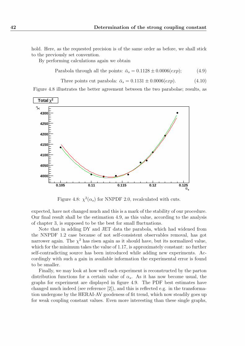
42 Determination of the strong coupling constant
hold. Here, as the requested precision is of the same order as before, we shall stickto the previously set convention.
By performing calculations again we obtain
Parabola through all the points: αs = 0.1128± 0.0006(exp); (4.9)
Three points cut parabola: αs = 0.1131± 0.0006(exp). (4.10)
Figure 4.8 illustrates the better agreement between the two parabolae; results, as
sα 0.105 0.11 0.115 0.12 0.125
2 χ
4000
4050
4100
4150
4200
4250
4300
2χTotal
Figure 4.8: χ2(αs) for NNPDF 2.0, recalculated with cuts.
expected, have not changed much and this is a mark of the stability of our procedure.Our final result shall be the estimation 4.9, as this value, according to the analysisof chapter 3, is supposed to be the best for small fluctuations.
Note that in adding DY and JET data the parabola, which had widened fromthe NNPDF 1.2 case because of not self-consistent observables removal, has gotnarrower again. The χ2 has risen again as it should have, but its normalized value,which for the minimum takes the value of 1.17, is approximately constant: no furtherself-contradicting source has been introduced while adding new experiments. Ac-cordingly with such a gain in available information the experimental error is foundto be smaller.
Finally, we may look at how well each experiment is reconstructed by the partondistribution functions for a certain value of αs. As it has now become usual, thegraphs for experiment are displayed in figure 4.9. The PDF best estimates havechanged much indeed (see reference [2]), and this is reflected e.g. in the transforma-tion undergone by the HERAI-AV goodeness of fit trend, which now steadily goes upfor weak coupling constant values. Even more interesting than these single graphs,
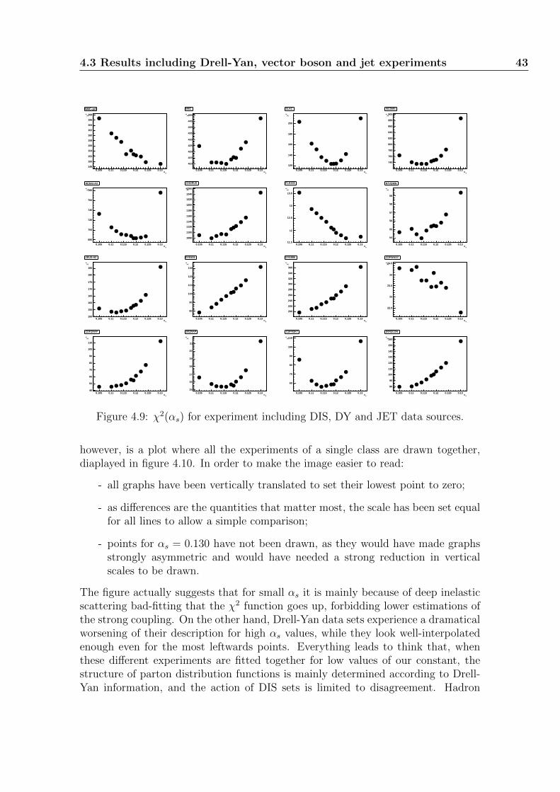
4.3 Results including Drell-Yan, vector boson and jet experiments 43
sα 0.105 0.11 0.115 0.12 0.125 0.13
2χ
148
150
152
154
156
158
160
162
164
166
168
NMC-pd
sα 0.105 0.11 0.115 0.12 0.125 0.13
2χ
410
415
420
425
430
435
440
445
450
NMC
sα 0.105 0.11 0.115 0.12 0.125 0.13
2χ
120
140
160
180
200
SLAC
sα 0.105 0.11 0.115 0.12 0.125 0.13
2χ
740
760
780
800
820
840
860
880
900
BCDMS
sα 0.105 0.11 0.115 0.12 0.125 0.13
2χ
680
700
720
740
760
780
HERAI-AV
sα 0.105 0.11 0.115 0.12 0.125 0.13
2χ
1080
1100
1120
1140
1160
1180
1200
1220
1240
1260
CHORUS
sα 0.105 0.11 0.115 0.12 0.125 0.13
2χ
11.5
12
12.5
13
13.5
FLH108
sα 0.105 0.11 0.115 0.12 0.125 0.13
2χ
54
55
56
57
58
59
NTVDMN
sα 0.105 0.11 0.115 0.12 0.125 0.13
2χ
150
155
160
165
170
175
180
185
ZEUS-H2
sα 0.105 0.11 0.115 0.12 0.125 0.13
2χ
80
90
100
110
120
130
DYE605
sα 0.105 0.11 0.115 0.12 0.125 0.13
2χ
200
220
240
260
280
300
320
340
360
DYE886
sα 0.105 0.11 0.115 0.12 0.125 0.13
2χ
22.5
23
23.5
24
24.5
CDFWASY
sα 0.105 0.11 0.115 0.12 0.125 0.13
2χ
40
50
60
70
80
90
100
110
CDFZRAP
sα 0.105 0.11 0.115 0.12 0.125 0.13
2χ
15
16
17
18
19
20
21
D0ZRAP
sα 0.105 0.11 0.115 0.12 0.125 0.13
2χ
60
70
80
90
100
110
CDFR2KT
sα 0.105 0.11 0.115 0.12 0.125 0.13
2χ
80
90
100
110
120
130
140
150
160
D0R2CON
Figure 4.9: χ2(αs) for experiment including DIS, DY and JET data sources.
however, is a plot where all the experiments of a single class are drawn together,diaplayed in figure 4.10. In order to make the image easier to read:
- all graphs have been vertically translated to set their lowest point to zero;
- as differences are the quantities that matter most, the scale has been set equalfor all lines to allow a simple comparison;
- points for αs = 0.130 have not been drawn, as they would have made graphsstrongly asymmetric and would have needed a strong reduction in verticalscales to be drawn.
The figure actually suggests that for small αs it is mainly because of deep inelasticscattering bad-fitting that the χ2 function goes up, forbidding lower estimations ofthe strong coupling. On the other hand, Drell-Yan data sets experience a dramaticalworsening of their description for high αs values, while they look well-interpolatedenough even for the most leftwards points. Everything leads to think that, whenthese different experiments are fitted together for low values of our constant, thestructure of parton distribution functions is mainly determined according to Drell-Yan information, and the action of DIS sets is limited to disagreement. Hadron
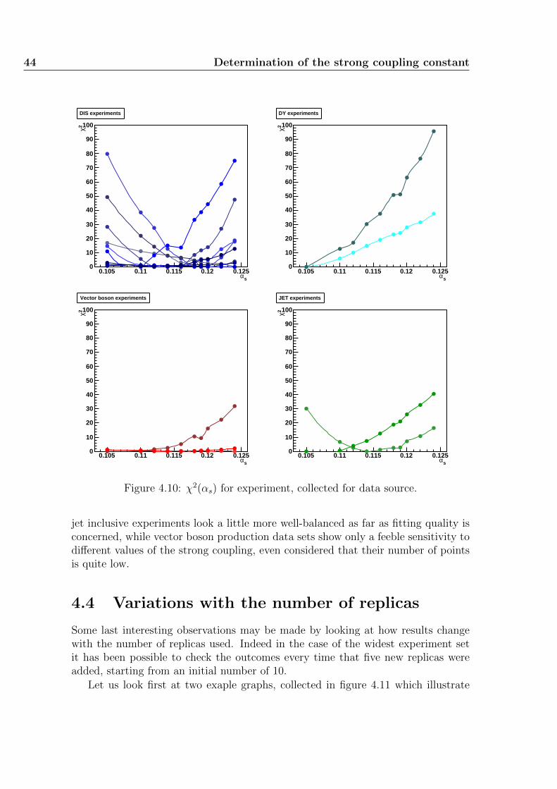
44 Determination of the strong coupling constant
sα 0.105 0.11 0.115 0.12 0.125
2 χ
0
10
20
30
40
50
60
70
80
90
100
DIS experiments
sα 0.105 0.11 0.115 0.12 0.125
2 χ
0
10
20
30
40
50
60
70
80
90
100
DY experiments
sα 0.105 0.11 0.115 0.12 0.125
2 χ
0
10
20
30
40
50
60
70
80
90
100
Vector boson experiments
sα 0.105 0.11 0.115 0.12 0.125
2 χ
0
10
20
30
40
50
60
70
80
90
100
JET experiments
Figure 4.10: χ2(αs) for experiment, collected for data source.
jet inclusive experiments look a little more well-balanced as far as fitting quality isconcerned, while vector boson production data sets show only a feeble sensitivity todifferent values of the strong coupling, even considered that their number of pointsis quite low.
4.4 Variations with the number of replicas
Some last interesting observations may be made by looking at how results changewith the number of replicas used. Indeed in the case of the widest experiment setit has been possible to check the outcomes every time that five new replicas wereadded, starting from an initial number of 10.
Let us look first at two exaple graphs, collected in figure 4.11 which illustrate
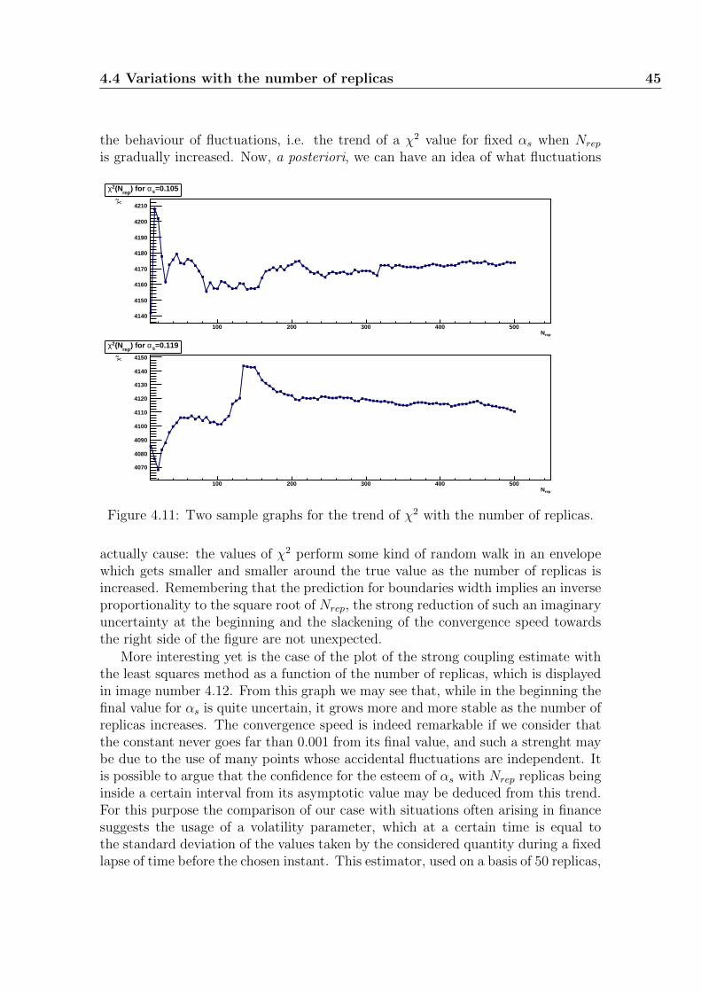
4.4 Variations with the number of replicas 45
the behaviour of fluctuations, i.e. the trend of a χ2 value for fixed αs when Nrep
is gradually increased. Now, a posteriori, we can have an idea of what fluctuations
repN100 200 300 400 500
2 χ
4140
4150
4160
4170
4180
4190
4200
4210
=0.105sα) for rep
(N2χ
repN100 200 300 400 500
2 χ
4070
4080
4090
4100
4110
4120
4130
4140
4150
=0.119sα) for rep
(N2χ
Figure 4.11: Two sample graphs for the trend of χ2 with the number of replicas.
actually cause: the values of χ2 perform some kind of random walk in an envelopewhich gets smaller and smaller around the true value as the number of replicas isincreased. Remembering that the prediction for boundaries width implies an inverseproportionality to the square root of Nrep, the strong reduction of such an imaginaryuncertainty at the beginning and the slackening of the convergence speed towardsthe right side of the figure are not unexpected.
More interesting yet is the case of the plot of the strong coupling estimate withthe least squares method as a function of the number of replicas, which is displayedin image number 4.12. From this graph we may see that, while in the beginning thefinal value for αs is quite uncertain, it grows more and more stable as the number ofreplicas increases. The convergence speed is indeed remarkable if we consider thatthe constant never goes far than 0.001 from its final value, and such a strenght maybe due to the use of many points whose accidental fluctuations are independent. Itis possible to argue that the confidence for the esteem of αs with Nrep replicas beinginside a certain interval from its asymptotic value may be deduced from this trend.For this purpose the comparison of our case with situations often arising in financesuggests the usage of a volatility parameter, which at a certain time is equal tothe standard deviation of the values taken by the considered quantity during a fixedlapse of time before the chosen instant. This estimator, used on a basis of 50 replicas,
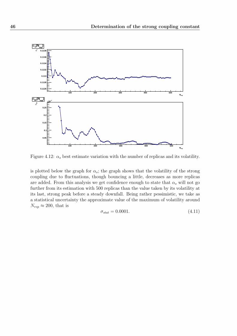
46 Determination of the strong coupling constant
repN100 200 300 400 500
sα
0.1126
0.1128
0.113
0.1132
0.1134
0.1136
0.1138
)rep
(Nsα
repN100 200 300 400 500
50σ
0.05
0.1
0.15
0.2
0.25
-310×)
rep(N50σ
Figure 4.12: αs best estimate variation with the number of replicas and its volatility.
is plotted below the graph for αs; the graph shows that the volatility of the strongcoupling due to fluctuations, though bouncing a little, decreases as more replicasare added. From this analysis we get confidence enough to state that αs will not gofurther from its estimation with 500 replicas than the value taken by its volatility atits last, strong peak before a steady downfall. Being rather pessimistic, we take asa statistical uncertainty the approximate value of the maximum of volatility aroundNrep ≈ 200, that is
σstat = 0.0001. (4.11)
Chapter 5
Conclusions and outlook
We have found that, in reproducing the correct behaviour of a function underlyinga point set affected by fluctuations the least squares method is usually the safestand most accurate. However, in the case of high fluctuations and good symmetryof the point set, applying the three points method with cuts results in more reliableoutcomes.
Concerning the determination of αs, we have found the value as an outcome of theNNPDF 1.2 analysis, but its comparison with a study based on the same DIS sourcesand performed with NNPDF 2.0 has shown that the former result is unreliablebecause of some faults in the older release of the fitting program. The estimationproduced by including Drell-Yan, vector boson production and jet inclusive data aswell as deep inelastic scattering experiments in the global fit is
αs = 0.1128± 0.0006(exp) ± 0.0001(stat).
This outcome is close to the DIS-only value, and yet more precise because it has awider empirical basis. The statistical uncertainty has been estimated by observingchanges in the αs estimation with the number of replicas used to obtain it.
However, a better solution for the determination of the statistical uncertaintyarises because we now have an idea for a possible computation of error bars uponχ2. The problem in finding confidence level intervals around the chi square foundvalue starting from the distribution of the same quantity for each replica is that thefinal value of χ2 is not the average of the single-replica χ2s, but rather the valueobtained computing the same function for the average PDF. These two operationsdo not commute, as the reconstruction of observables is a highly non-linear pro-cedure. Thus informations for different numbers of replicas are qualitatively veryunlike one another when the said numbers are not close. When the replicas setsinclude e.g. more than one hundred replicas each and a single replica separatesthem, the chi squares estimations they lead to cannot be that much different. Thisfeature becomes interesting when it is put together with the idea of the jackknifemethod The latter prescribes error computation for some kind of average of n quan-tities as the standard deviation of the n values obtained excluding one element at
48 Conclusions and outlook
a time, multiplied by√n in order to avoid the underestimation that comes from
subsets’ strong correlation. The combination of these two strategies could allow fora good estimation of uncertainties and then, because of this appropriate treatmentof fluctuations, for the application of more reliable, simple fitting techniques.
Another open question which needs an answer is the relationship of the twosuggested three-points methods’ estimations for the statistical error on αs with thewidth of the probability distribution functions obtained through the toy program;such a direct connection has indeed been looked for, but it has not been found yet.
A possible future development has to do with the mentioned conjectures whichhint for a possible problem with low Q2, low x data. An interesting step in thedirection of understanding this problem could be the application of kinematic cutsin that zone and the study of consequences upon the best αs value.
Last we shall say that in the meanwhile a new version of NNPDF, number 2.1,has been released. It features an improvement in heavy quark thresholds’ handling,and the stability of our result under such a change needs to be checked.
Bibliography
[1] R.D. Ball, L. Del Debbio, S. Forte, A. Guffanti, J.I. Latorre, A. Piccione, J. Rojo,and M. Ubiali, A determination of parton distributions with faithful uncertaintyestimation, Nuclear Physics B 809 (2009), no. 1-2, 1–63.
[2] R.D. Ball, L. Del Debbio, S. Forte, A. Guffanti, J.I. Latorre, J. Rojo, andM. Ubiali, A first unbiased global NLO determination of parton distributionsand their uncertainties, arXiv 1002.
[3] R. Brun and F. Rademakers, ROOT–An object oriented data analysis framework,Nuclear Instruments and Methods in Physics Research Section A: Accelerators,Spectrometers, Detectors and Associated Equipment 389 (1997), no. 1-2, 81–86.
[4] G.D. Coughlan and J.E. Dodd, The ideas of particle physics: an introductionfor scientists, Cambridge Univ Pr, 1991.
[5] G. Cowan, Statistical data analysis, Oxford University Press, USA, 1998.
[6] A. Das and T. Ferbel, Introduction to nuclear and particle physics, World Scien-tific Pub Co Inc, 2003.
[7] E. Mariani, Determination of the strong coupling from an unbiased global partonfit, Undergraduate Thesis, Milan University (2009).
[8] K. Nakamura and (Particle Data Group), J. Phys. G: Nucl. Part. Phys. 37(2010).


![arXiv:1605.05541v1 [hep-ph] 18 May 20161 Introduction Deep-inelastic scattering provides one of the most direct methods to measure the strong coupling constant from precision data](https://static.fdocument.org/doc/165x107/60bb6787511ed5109750f235/arxiv160505541v1-hep-ph-18-may-2016-1-introduction-deep-inelastic-scattering.jpg)


![Determination of the strong coupling constant from transverse … · 2018. 1. 17. · [850,900] 1240059 437 [900,1000] 1465814 472 [1000,1100] 745898 522 [1100,1400] 740563 604 [1400,5000]](https://static.fdocument.org/doc/165x107/60c7fdfd0110035e8422cb49/determination-of-the-strong-coupling-constant-from-transverse-2018-1-17-850900.jpg)