Microwave fidelity studies by varying antenna coupling
22
Microwave fidelity studies by varying antenna coupling Hans-J ¨ urgen St ¨ ockmann [email protected] Fachbereich Physik, Philipps-Universit ¨ at Marburg, D-35032 Marburg, Germany [B. K ¨ ober, U. Kuhl, H.-J. St., T. Gorin, T. Seligman, D. Savin, PRE 82, 036207 (2010)] Marburg, May 2010 – p.
Transcript of Microwave fidelity studies by varying antenna coupling
Microwave fidelity studies by varyingantenna coupling
Hans-Jurgen Stockmann
Fachbereich Physik, Philipps-Universitat Marburg, D-35032 Marburg, Germany
[B. Kober, U. Kuhl, H.-J. St., T. Gorin, T. Seligman, D. Savin, PRE 82, 036207 (2010)]
Marburg, May 2010 – p.
Fidelity
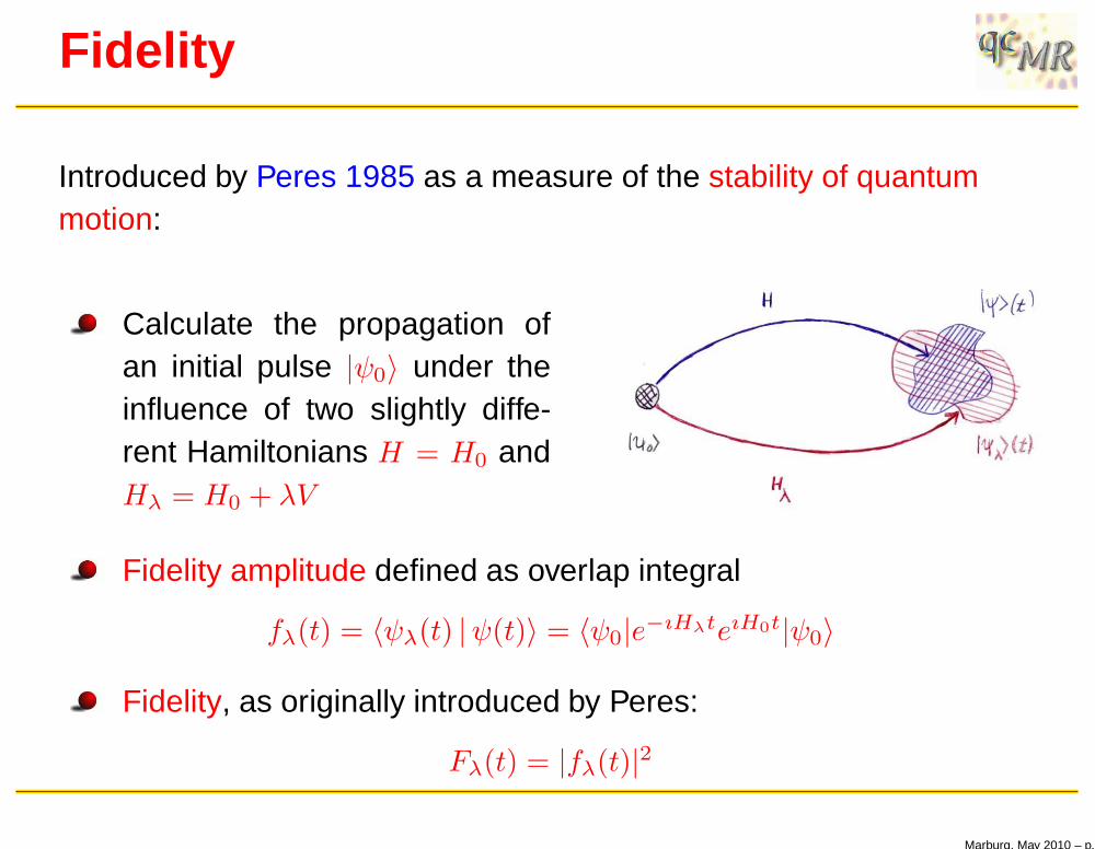
Introduced by Peres 1985 as a measure of the stability of quantummotion:
Calculate the propagation ofan initial pulse |ψ0〉 under theinfluence of two slightly diffe-rent Hamiltonians H = H0 andHλ = H0 + λV
Fidelity amplitude defined as overlap integral
fλ(t) = 〈ψλ(t) |ψ(t)〉 = 〈ψ0|e−ıHλteıH0t|ψ0〉
Fidelity, as originally introduced by Peres:
Fλ(t) = |fλ(t)|2
Marburg, May 2010 – p.
Experimental realisations
Spin-Echo experiments in NMR (Levstein, Usaj, Pastawski 1998)
Measures the nuclear magnetisation averaged over the wholesample forward and backward in time is measured!
But wave functions are not accessible!
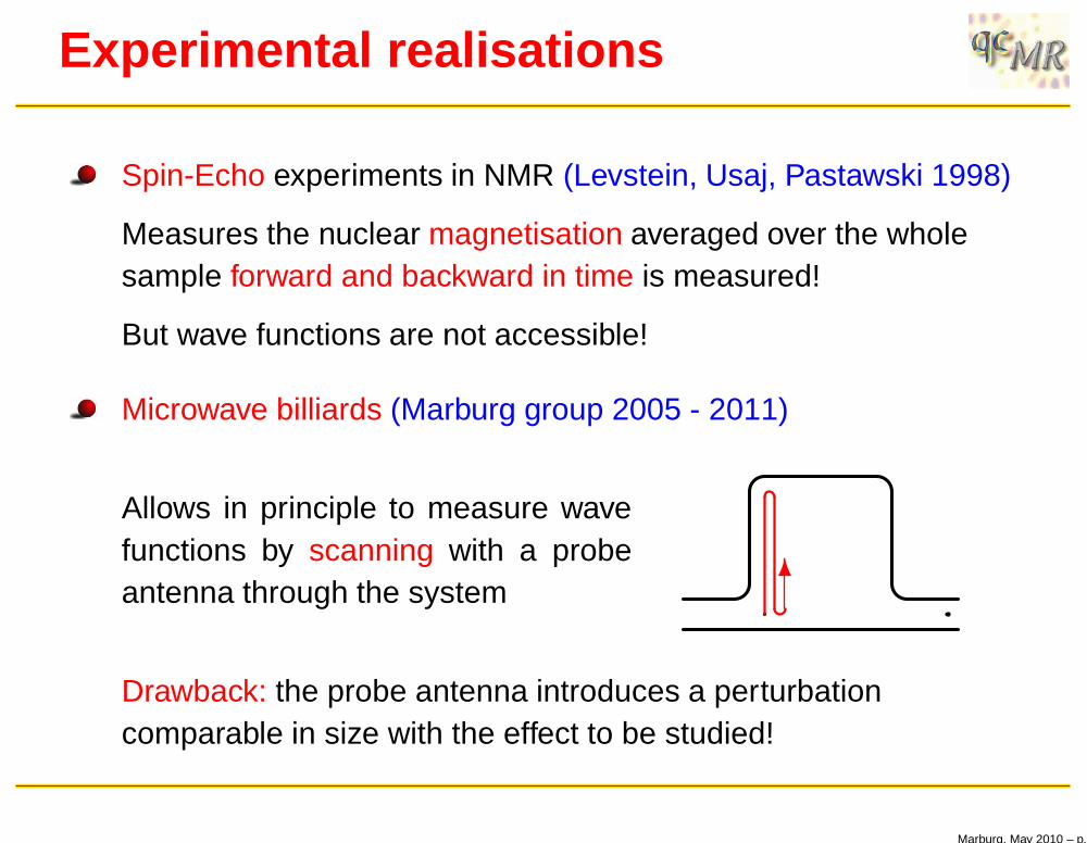
Microwave billiards (Marburg group 2005 - 2011)
Allows in principle to measure wavefunctions by scanning with a probeantenna through the system 6
Drawback: the probe antenna introduces a perturbationcomparable in size with the effect to be studied!
Marburg, May 2010 – p.
Scattering matrix
6?- aiR
Ibibn =
∑
m
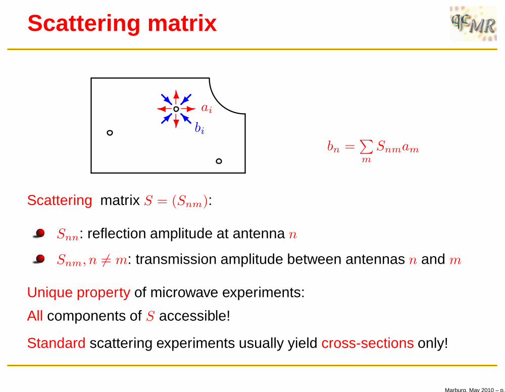
Snmam
Scattering matrix S = (Snm):
Snn: reflection amplitude at antenna n
Snm, n 6= m: transmission amplitude between antennas n and m
Unique property of microwave experiments:
All components of S accessible!
Standard scattering experiments usually yield cross-sections only!
Marburg, May 2010 – p.
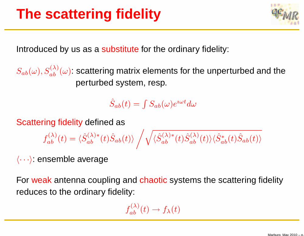
The scattering fidelity
Introduced by us as a substitute for the ordinary fidelity:
Sab(ω), S(λ)ab (ω): scattering matrix elements for the unperturbed and the
perturbed system, resp.
Sab(t) =∫
Sab(ω)eıωtdω
Scattering fidelity defined as
f(λ)ab (t) = 〈S(λ)∗
ab (t)Sab(t)〉/
√
〈S(λ)∗ab (t)S
(λ)ab (t)〉〈S∗
ab(t)Sab(t)〉
〈· · ·〉: ensemble average
For weak antenna coupling and chaotic systems the scattering fidelityreduces to the ordinary fidelity:
f(λ)ab (t) → fλ(t)
Marburg, May 2010 – p.
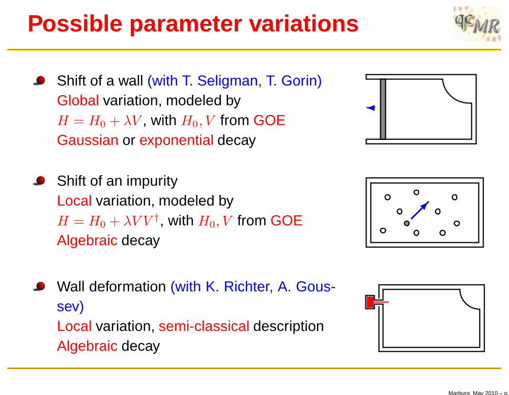
Possible parameter variations
Shift of a wall (with T. Seligman, T. Gorin)Global variation, modeled byH = H0 + λV , with H0, V from GOEGaussian or exponential decay
Shift of an impurityLocal variation, modeled byH = H0 + λV V †, with H0, V from GOEAlgebraic decay
Wall deformation (with K. Richter, A. Gous-sev)Local variation, semi-classical descriptionAlgebraic decay
Marburg, May 2010 – p.
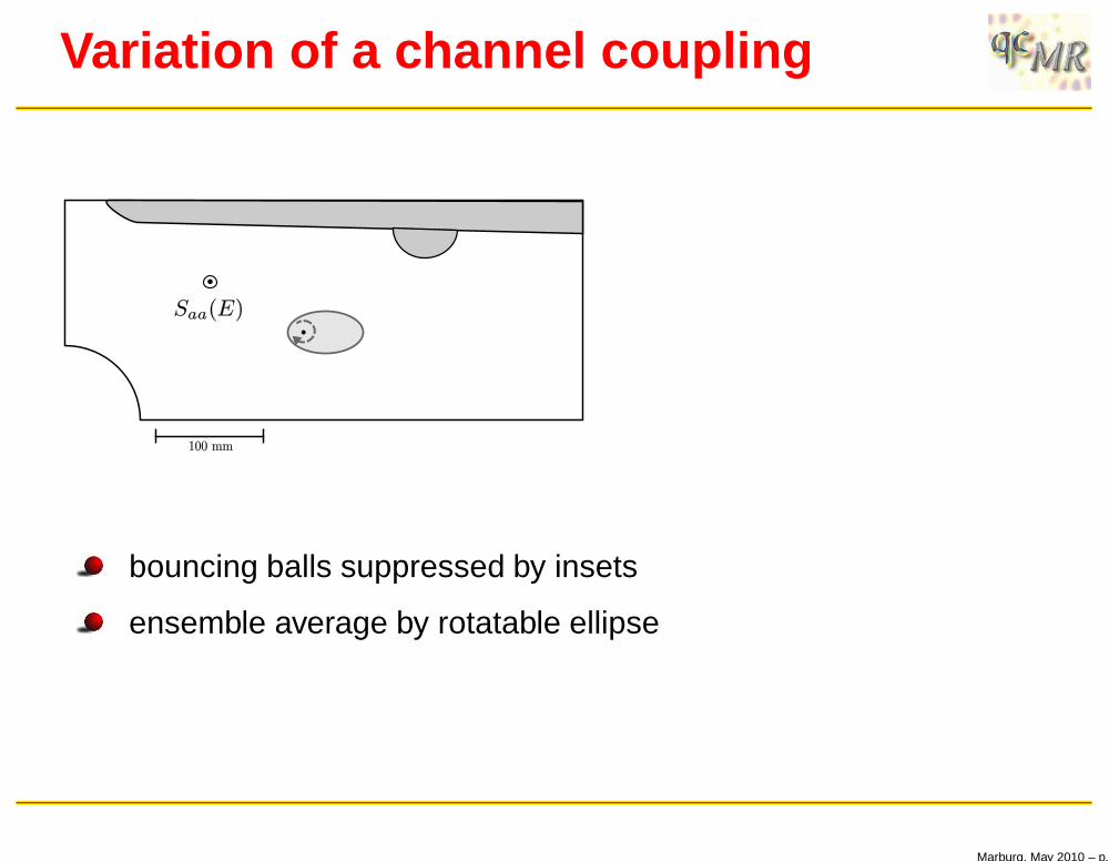
Variation of a channel coupling
bouncing balls suppressed by insets
ensemble average by rotatable ellipse
Marburg, May 2010 – p.
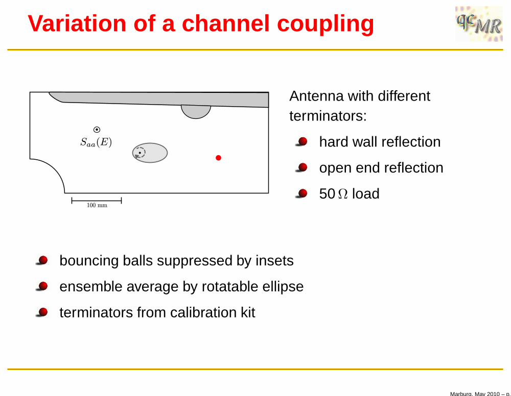
Variation of a channel coupling
•
Antenna with differentterminators:
hard wall reflection
open end reflection
50 Ω load
bouncing balls suppressed by insets
ensemble average by rotatable ellipse
terminators from calibration kit
Marburg, May 2010 – p.
The effective Hamiltonian
6?- aiR
Ibibn =
∑
m
Snmam
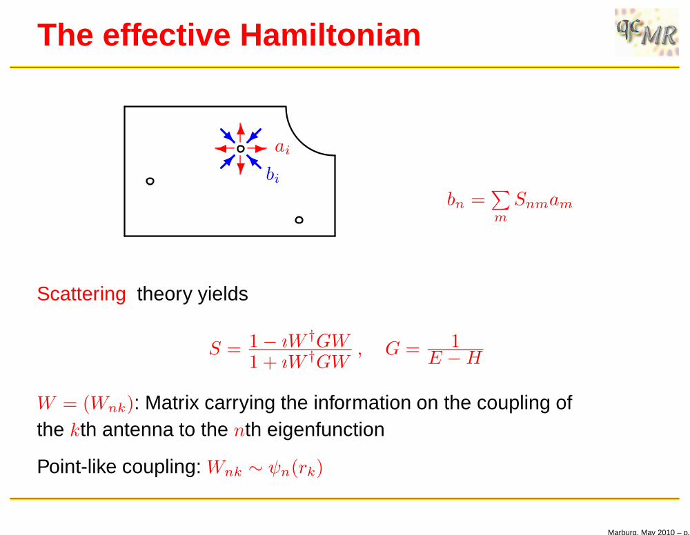
Scattering theory yields
S = 1 − ıW †GW1 + ıW †GW
, G = 1E −H
W = (Wnk): Matrix carrying the information on the coupling ofthe kth antenna to the nth eigenfunction
Point-like coupling: Wnk ∼ ψn(rk)
Marburg, May 2010 – p.
The effective Hamiltonian ( cont.)
•
bA
bC
=
SAA SAC
SCA SCC
aA
aC
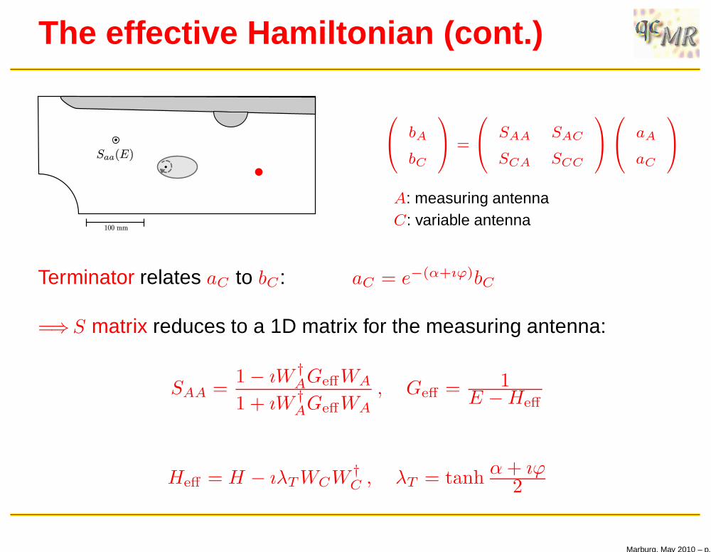
A: measuring antennaC: variable antenna
Terminator relates aC to bC : aC = e−(α+ıϕ)bC
=⇒S matrix reduces to a 1D matrix for the measuring antenna:
SAA =1 − ıW †
AGeffWA
1 + ıW †AGeffWA
, Geff = 1E −Heff
Heff = H − ıλTWCW†C , λT = tanh
α+ ıϕ2
Marburg, May 2010 – p.
The effective Hamiltonian ( cont.)
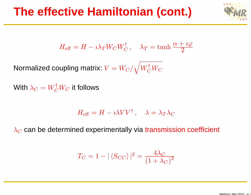
Heff = H − ıλTWCW†C , λT = tanh α+ ıϕ
2
Normalized coupling matrix: V = WC/√
W †CWC
With λC = W †CWC it follows
Heff = H − ıλV V † , λ = λTλC
λC can be determined experimentally via transmission coefficient
TC = 1 − | 〈SCC〉 |2 = 4λC
(1 + λC)2
Marburg, May 2010 – p. 10
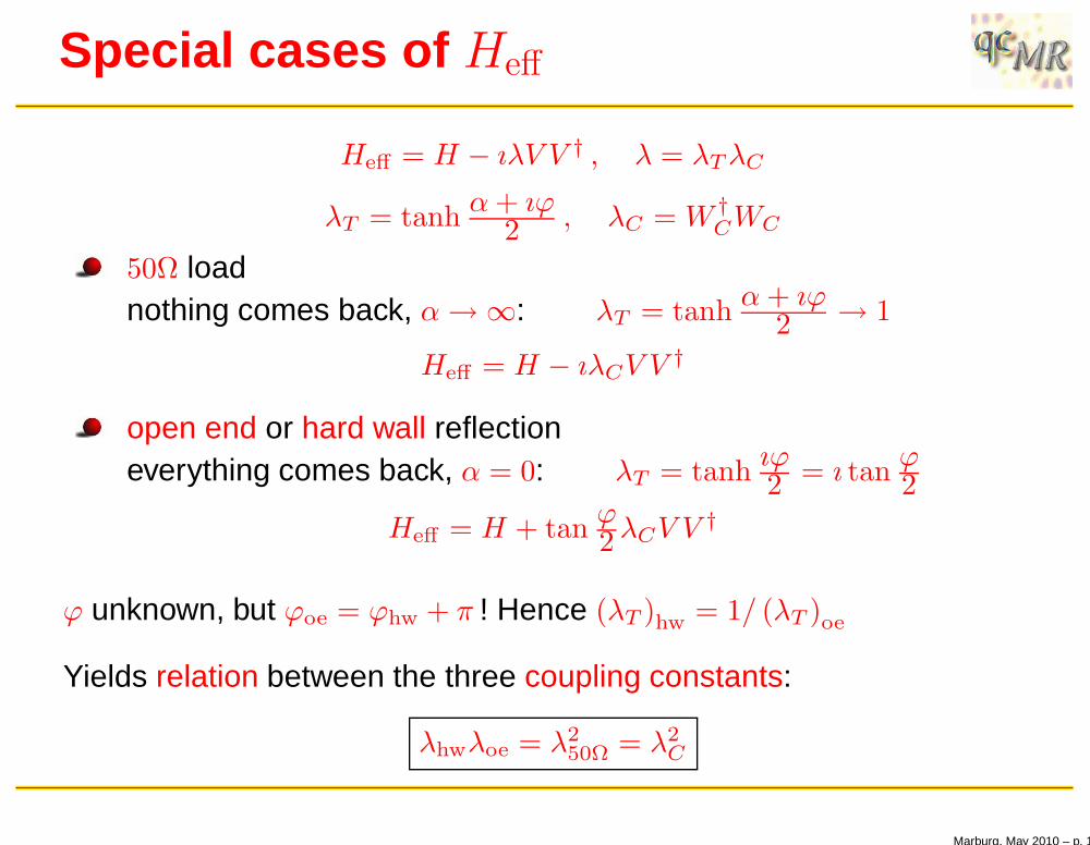
Special cases of Heff
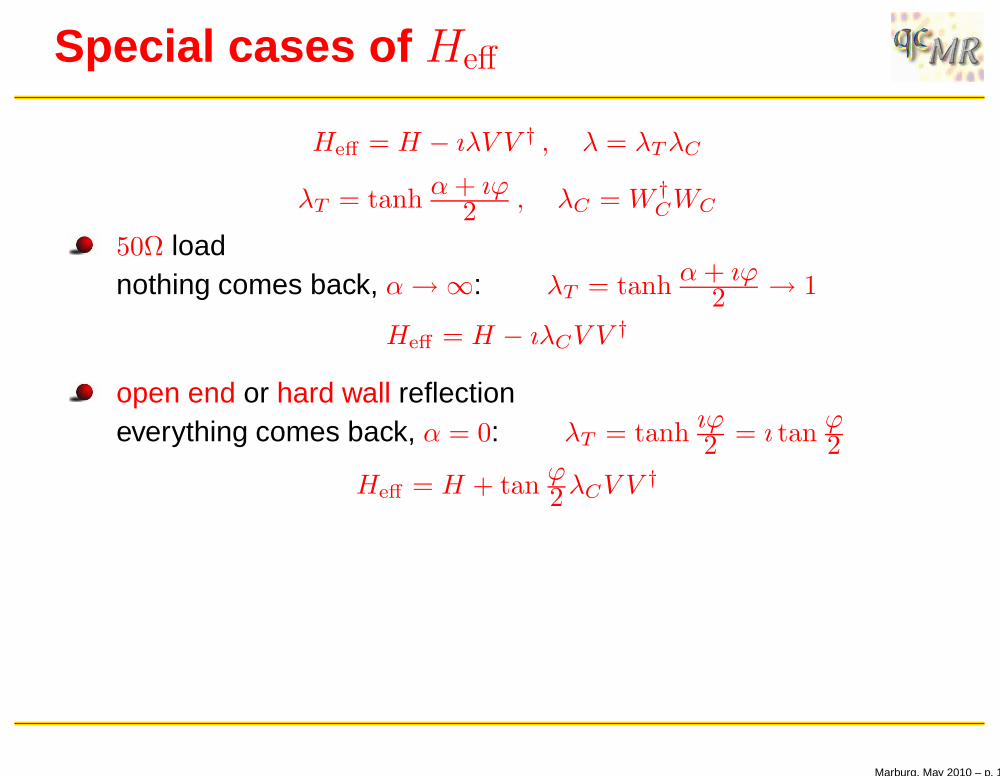
Heff = H − ıλV V † , λ = λTλC
λT = tanh α+ ıϕ2 , λC = W †
CWC
50Ω loadnothing comes back, α→ ∞: λT = tanh
α+ ıϕ2 → 1
Heff = H − ıλCV V†
open end or hard wall reflectioneverything comes back, α = 0: λT = tanh
ıϕ2 = ı tan
ϕ2
Heff = H + tanϕ2 λCV V
†
Marburg, May 2010 – p. 11
Special cases of Heff
Heff = H − ıλV V † , λ = λTλC
λT = tanh α+ ıϕ2 , λC = W †
CWC
50Ω loadnothing comes back, α→ ∞: λT = tanh
α+ ıϕ2 → 1
Heff = H − ıλCV V†
open end or hard wall reflectioneverything comes back, α = 0: λT = tanh
ıϕ2 = ı tan
ϕ2
Heff = H + tanϕ2 λCV V
†
ϕ unknown, but ϕoe = ϕhw + π ! Hence (λT )hw = 1/ (λT )oe
Yields relation between the three coupling constants:
λhwλoe = λ250Ω = λ2
C
Marburg, May 2010 – p. 11
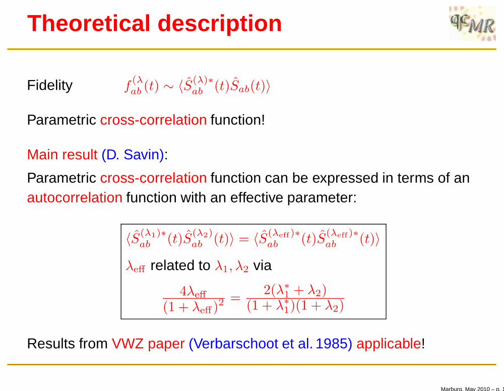
Theoretical description
Fidelity f(λab (t) ∼ 〈S(λ)∗
ab (t)Sab(t)〉
Parametric cross-correlation function!
Main result (D. Savin):
Parametric cross-correlation function can be expressed in terms of anautocorrelation function with an effective parameter:
〈S(λ1)∗ab (t)S
(λ2)ab (t)〉 = 〈S(λeff)∗
ab (t)S(λeff)∗ab (t)〉
λeff related to λ1, λ2 via
4λeff
(1 + λeff)2=
2(λ∗1 + λ2)(1 + λ∗1)(1 + λ2)
Results from VWZ paper (Verbarschoot et al. 1985) applicable!
Marburg, May 2010 – p. 12
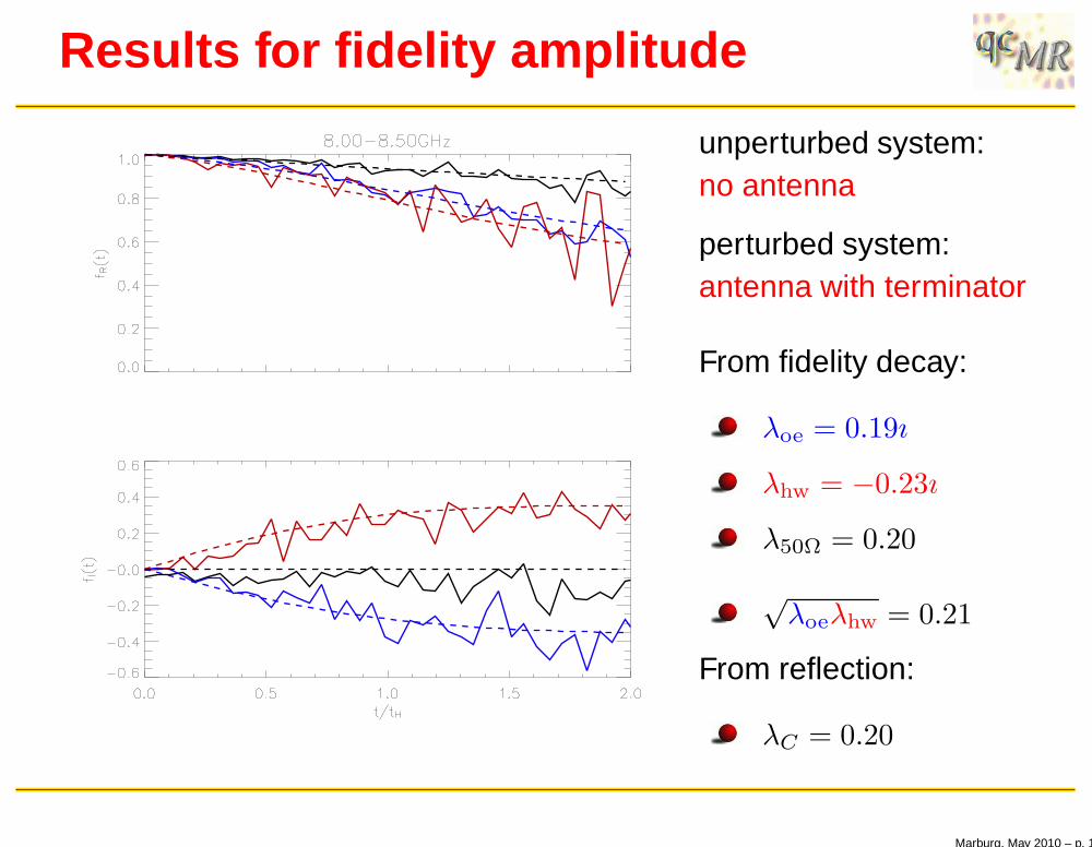
Results for fidelity amplitude
unperturbed system:no antenna
perturbed system:antenna with terminator
From fidelity decay:
λoe = 0.19ı
λhw = −0.23ı
λ50Ω = 0.20
√λoeλhw = 0.21
From reflection:
λC = 0.20
Marburg, May 2010 – p. 13
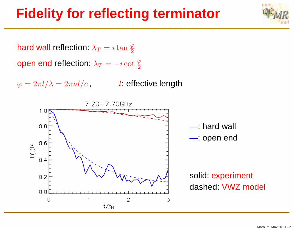
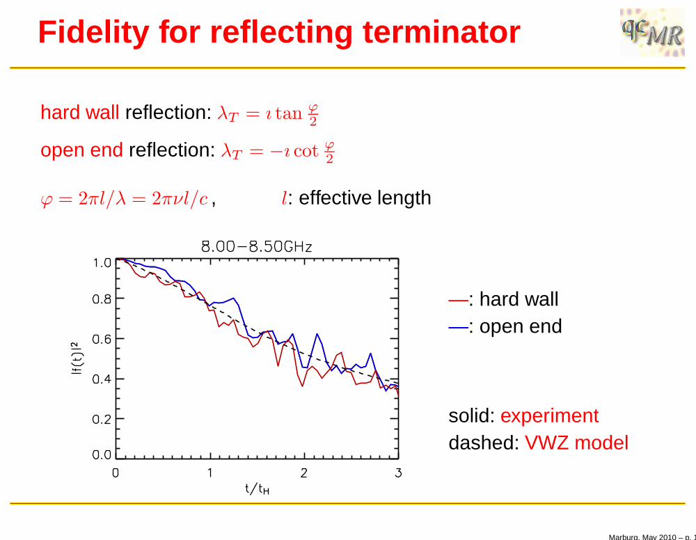
Fidelity for reflecting terminator
hard wall reflection: λT = ı tan ϕ2
open end reflection: λT = −ı cot ϕ2
ϕ = 2πl/λ = 2πνl/c , l: effective length
—: hard wall—: open end
solid: experimentdashed: VWZ model
Marburg, May 2010 – p. 14
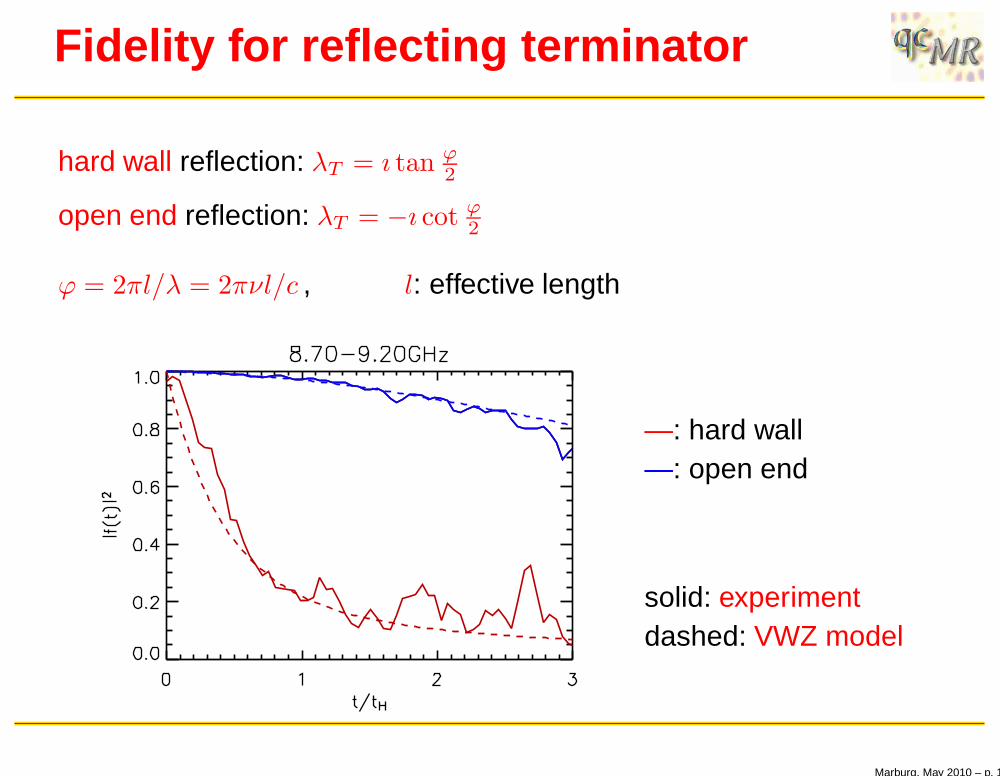
Fidelity for reflecting terminator
hard wall reflection: λT = ı tan ϕ2
open end reflection: λT = −ı cot ϕ2
ϕ = 2πl/λ = 2πνl/c , l: effective length
—: hard wall—: open end
solid: experimentdashed: VWZ model
Marburg, May 2010 – p. 14
Fidelity for reflecting terminator
hard wall reflection: λT = ı tan ϕ2
open end reflection: λT = −ı cot ϕ2
ϕ = 2πl/λ = 2πνl/c , l: effective length
—: hard wall—: open end
solid: experimentdashed: VWZ model
Marburg, May 2010 – p. 14
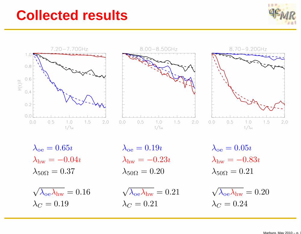
Collected results
λoe = 0.65ı
λhw = −0.04ı
λ50Ω = 0.37
√λoeλhw = 0.16
λC = 0.19
λoe = 0.19ı
λhw = −0.23ı
λ50Ω = 0.20
√λoeλhw = 0.21
λC = 0.21
λoe = 0.05ı
λhw = −0.83ı
λ50Ω = 0.21
√λoeλhw = 0.20
λC = 0.24
Marburg, May 2010 – p. 15
Conclusions
Description of the billiard with variable antenna in terms of aneffective Hamiltonian
Explicit expressions of the coupling parameters in terms ofterminator properties
Description of the scattering fidelity, a parametric cross-correlationfunction, in terms of an autocorrelation function with an effectiveparameter, thus reduction to the VWZ problem
Quantitative agreement between experiment and theory
Marburg, May 2010 – p. 16
Conclusions
Description of the billiard with variable antenna in terms of aneffective Hamiltonian
Explicit expressions of the coupling parameters in terms ofterminator properties
Description of the scattering fidelity, a parametric cross-correlationfunction, in terms of an autocorrelation function with an effectiveparameter, thus reduction to the VWZ problem
Quantitative agreement between experiment and theory
General problem:
Fidelity decays for closed and open systems hardly discernible
Reliable results only for a perfectly controllable situation
Usually an open channel simultaneously acts as a scatterer
Marburg, May 2010 – p. 16
Thanks!
Coworkers:
B. KöberU. Kuhl
Cooperations:
T. Gorin, Guadalajara, MexicoT. Seligman, Cuernavaca, MexicoD. Savin, Brunel, UK
The experiments have been supported by the DFG via the
FG 760 “Scattering Systems with Complex Dynamics”.
Marburg, May 2010 – p. 17