arX

iv:h

ep-p

h/04

0916

9v2

27

Jan

2007

FT–2004–03Caltech MAP–300

The Weak Mixing Angle at Low Energies

Jens Erler1

and Michael J. Ramsey-Musolf2

1Instituto de Fısica, Universidad Nacional Autonoma de Mexico, 01000 Mexico D.F., Mexico

2Kellogg Radiation Laboratory, California Institute of Technology, Pasadena, CA 91125, USA

Abstract

We determine the weak mixing angle in the MS-scheme, sin2 θW (µ), at energy scalesµ relevant for present and future low energy electroweak measurements. We relate therenormalization group evolution of sin2 θW (µ) to the corresponding evolution of α(µ) andinclude higher-order terms in αs and α that had not been treated in previous analyses. Wealso up-date the analysis of non-perturbative, hadronic contributions and argue that theassociated uncertainty is small compared to anticipated experimental errors. The resultingvalue of the low-energy MS weak mixing angle is sin2 θW (0) = 0.23867 ± 0.00016.

1 Introduction

The weak mixing angle is one of the fundamental parameters of the electroweak Standard Model(SM). It can be defined through the relation,

sin2 θW =g′2

g2 + g′2, (1)

where g and g′ are the SU(2)L and U(1)Y gauge couplings, respectively. Its value is not predictedand needs to be extracted from parity violating neutral current experiments, where by far themost precise results were obtained at the Z factories LEP 1 and SLC. Electroweak symmetrybreaking provides masses for the W and Z bosons proportional to their gauge interactions.Therefore, one has the additional relation,

sin2 θW = 1 − M2W

M2Z

, (2)

and the gauge boson mass ratio provides independent precise information on sin2 θW . Extractingthe fine structure constant,

α =e2

4π=

g2 sin2 θW

4π, (3)

from the quantum Hall effect or the anomalous magnetic moment of the electron, then fixes bothgauge couplings. Eqs. (1) and (3) are valid at the tree level and modified by radiative corrections.

1

As a result, the precise numerical value of sin2 θW depends on the renormalization scheme andscale chosen. For example, the on-shell renormalization scheme promotes Eq. (2) to a definitionof sin2 θW ≡ sin2 θ on−shell

W to all orders in perturbation theory. This definition has the advantageof being directly related to a physical observable — but only to one-loop order. Since the gaugebosons are unstable particles their masses become ambiguous starting at two-loop precision.

As an alternative, one can define flavor-dependent “effective” mixing angles appearing in theZ vector coupling1,

vf = Tf − 2Qf sin2 θ efff , (4)

where Qf and Tf are the fermion charge and third component of isospin, respectively. Gaugeboson self-energy and Zff -vertex corrections are absorbed into scheme dependent form factors,ρf and κf that are equal to unity at tree-level. The ρf are corrections to the overall couplingstrengths and the κf are defined by,

sin2 θ efff ≡ κf sin2 θ on−shell

W ≡ κf sin2 θW (MZ), (5)

where the caret marks quantities in the modified minimal subtraction (MS) scheme [2–4]. Thiseffective sin2 θ eff

f is a useful definition as long as electroweak box contributions can be neglected;since these do not resonate this condition is clearly satisfied at LEP 1 and SLC. However, withthe greater precision that could be achieved with the GigaZ option of TESLA, such boxes couldbecome non-negligible. Thus, it is not easy to construct a definition that can be equated toa physical observable to all orders. Neither is this of practical relevance: as long as it is well-defined, sin2 θW can be looked upon as a mere bookkeeping device and means to compare variousexperimental results.

What is of practical importance, however, is the numerical value of the mixing angle usedin computing a given observable in a specified renormalization scheme. Generally speaking, oneexpects a one-loop radiatively corrected result to be valid up to small corrections of O( α2

π2 sin4 θW) ∼

10−4. On the other hand, for leptons we have,

(κℓ − 1)2 ≈ 1.5 × 10−3, (6)

which is not much smaller than a typical one-loop contribution. The reason is that κℓ containstop-quark mass enhancements factors, m2

t /M2W , that spoil the expected behavior of the pertur-

bation series. Fortunately, such enhancement factors can be avoided by a judicious choice ofdefinition of the weak mixing angle (or renormalization scheme), rendering the truncation errorsmall. The MS-definition considered in this article has this property, except that small ln m2

t /M2W

corrections cannot be decoupled simultaneously from all observables [5,6].For processes off the Z-pole, enhancement factors of similar magnitude as those entering

Eq. (6) can arise from large logarithms lnM2Z/m2

f , where mf is some fermion mass. Thesecan occur even within a specifically chosen renormalization scheme. Typically, such logarithms

1We normalize vf without an additional factor inversely proportional to sin θW cos θW . The scale in this factorneeds to be chosen of electroweak size, µ = MZ , even for low energy processes. This is automatically achievedby normalizing neutral-current amplitudes using ρ GF , where GF is the Fermi constant and ρ the low energyneutral-current ρ parameter [1] (which is free of fermionic mass singularities). Thus, this factor does not affectour discussion.

2

are artifacts of using a value for sin2 θW obtained at the Z scale (where as noted above, it ismeasured very precisely) in theoretical expressions for very low (or high) energy observables. Insome renormalization schemes, the weak mixing angle depends explicitly on a renormalizationscale parameter, which could be the t’Hooft scale, µ, appearing in dimensional regularization,or the momentum transfer q2. For others there is no explicit scale parameter, and the scaledependence is of indirect nature. In either case, the aforementioned logarithms are a potentialhazard and should be avoided or re-summed if possible.

The main goal of this paper is to present an analysis of the weak mixing angle in the MS-scheme, sin2 θW (0), relevant for observables measured at (almost) vanishing momentum transfer.These observables include the nuclear weak charge obtained in the well-known cesium atomicparity violation measurement performed by the Boulder group [7]; the parity violating Møllerasymmetry at SLAC [8]; and the up-coming measurement of the weak charge of the proton at Jef-ferson Lab [9]. Precision measurements of the parity violating deep inelastic eD asymmetry havealso been discussed as future possibilities for Jefferson Lab, as has a more precise measurementof the Møller asymmetry. The value of sin2 θW (0) is particularly relevant for the interpretationof the parity violation experiments, since the vector coupling of the Z n Eq. (4) to electrons andprotons is proportional to 1−4 sin2 θW (q2)eff

f ∼ 0.1 and is, therefore, highly sensitive to the valueof the effective weak mixing angle. Indeed, as noted in Refs. [10,11], one-loop contributions tosin2 θW (0)eff

f reduce the magnitude of the Møller asymmetry by roughly 40% from its tree-levelvalue, an effect generated by the large logarithms discussed above. Moreover, the presence ofthese large logarithms in sin2 θW (0)eff

f is universal to all low energy neutral current observables,though their net effect may be masked by other enhanced radiative corrections2. Consequently,one would like to sum these universally enhanced contributions to all orders. Here, we do sousing the renormalization group evolution for sin2 θW (µ) in the MS-scheme.

The MS-definition of the weak mixing angle is, of course, not unique, and one may choosean alternate scheme in which to compute radiative corrections to electroweak observables. Nev-ertheless, the MS-scheme offers several advantages that motivate our adoption of it here. Inparticular, the MS-definition of sin2 θW (µ) follows closely the coupling-based definition in Eq. (1)with a well-defined subtraction of singular terms arising in dimensional regularization, giving riseto expressions with a logarithmic µ-dependence. This dependence is governed by a renormal-ization group equation (RGE), and choosing µ equal to the momentum transfer of the processunder consideration will in general avoid spurious logarithms3. As we discuss below, the evolu-tion of sin2 θW (µ) can be related in a straightforward way to that of α(µ), the QED coupling inthe MS-scheme that has been thoroughly studied elsewhere. Doing so allows us to draw uponknown results for the QED β-function and – in conjunction with suitable matching conditions –to improve the precision of the Standard Model predictions for low-energy observables by incor-porating various higher order effects. Indeed, although the one-loop RGE for sin2 θW (µ) has beenwell-studied by others, one emphasis of the present work is the inclusion of higher order QEDand perturbative QCD contributions in a systematic way. We discuss the RGE in Sections 2

2 For example, the left-right asymmetry for parity-violating elastic ep scattering also contains large logarithmsassociated with the fermion anapole moment as well as non-logarithmic but large WW box graphs [12,13,14].

3The presence of some logarithmically-enhanced radiative corrections, such as the anapole moment effects,cannot be cannot be eliminated by the RGE for sin2 θW (µ).

3

and 3, and matching conditions in Section 4.A major complication arises when the contribution of the light quark flavors is considered for µ

of order a hadronic scale, Λ, or smaller. In this regime, QCD corrections to the RGE (β-function)cannot be obtained using perturbative methods. An analogous problem is well-known to arisefor α(µ) when its value is desired at scales similar to or greater than Λ. We address this problemin Sections 5 and 6, as well as two appendices. We argue that the corresponding theoreticaluncertainty is well below the anticipated experimental errors and provide a new estimate ofthis uncertainty that is substantially smaller in magnitude than the previously-quoted one [15].Non-logarithmic contributions and some more formal aspects are discussed in Section 7 while

numerical results and a plot of sin2 θW (µ) for µ =√

|q2| – along with conclusions – are presentedin Section 8. We note there our results may also be applied to the recent studies of deep-inelasticneutrino-nucleus scattering carried out by the NuTeV Collaboration [16].

2 Leading order RGE analysis

The quantity sin2 θW (0) is related to s2Z ≡ sin2 θW (MZ) by,

sin2 θW (0) ≡ κ(0) sin2 θW (MZ) ≡ [1 + ∆κ(0)]s2Z , (7)

where ∆κ(0) is a universal (flavor-independent) radiative correction. In this Section we areinterested in logarithmic contributions to κ(0) of the form,

α

π sin2 θW

lnM2

Z

m2i

,

and in particular in the scale that should be used in α and sin2 θW , appropriate for re-summingthe leading, large logarithms to all orders. These logarithms arise from scale dependent self-energy mixing diagrams where one external leg is a photon and the other one is a Z-boson.Thus, vf acquires a compensating scale dependence,

vf

(

√

µ2 + ∆µ2

)

= vf (µ) +α(µ)

24πQf

∑

i

[N ci γivi(µ)Qi] ln

µ2 + ∆µ2

µ2, (8)

where N cq = NC = 3 (for quarks) and N c

ℓ = 1 (for leptons) is the color factor. We have writtenthe sum in general form to also allow chiral fermions and bosonic degrees of freedom (to putthe W± and Higgs ghosts on the same footing as the fermions and to facilitate the discussion inSection 7), where the spin dependent factors γi are shown in Table 1. With these conventions,the factor of 1/24 also appears in the lowest order QED β-function coefficient,

µ2 dα

dµ2=

α2

24π

∑

i

N ci γiQ

2i . (9)

This implies the RGE,

µ2 dvf

dµ2=

α

24πQf

∑

i

N ci γiviQi, (10)

4

field γi

real scalar 1complex scalar 2chiral fermion 4Majorana fermion 4Dirac fermion 8massless gauge boson −22

Table 1: Weight factors γi entering the leading RGE coefficients for the weak mixing angle.

or in terms of the variable X =∑

i Nci γiviQi,

dX

X=

α

24π

dµ2

µ2

∑

i

N ci γiQ

2i =

dα

α, (11)

where in the second equality we used Eq. (9). This is solved by,

sin2 θW (µ) =α(µ)

α(µ0)sin2 θW (µ0) +

∑

i Nci γiQiTi

∑

i Nci γiQ2

i

[

1 − α(µ)

α(µ0)

]

, (12)

or using the explicit solution to the one-loop RGE in Eq. (9) we obtain the simpler form,

sin2 θW (µ) = sin2 θW (µ0)

[

1 +α(µ)

24π sin2 θW (µ0)

∑

i

N ci γiQi[Ti − Qi sin

2 θW (µ0)] lnµ2

0

µ2

]

. (13)

The result in Eq. (13) re-sums all logarithms of O(αn lnn µ0

µ) provided there is no particle

threshold between µ and µ0. To avoid reintroduction of spurious logarithms this solution mustbe applied successively from one particle threshold to the next. Crossing a threshold from above,the corresponding particle is integrated out, and one continues with an effective field theorywithout this particle. In contrast, changing from one effective field theory to another far awayfrom the physical mass of the particle would not formally affect the truncated one-loop result,but it would spoil its re-summation.

Eq. (13) applied to ∆κ(0) can be brought into the well-known form [14],

∆κ(0) =α

πs2Z

1

6

∑

f

N cfQf (Tf − 2Qf s

2Z) ln

M2Z

m2f

−(

43

24− 7

4s2

Z

)

lnM2

Z

M2W

, (14)

where the sum is over all SM Dirac fermions excluding the top quark. The last term is the W±

contribution with its coefficient obtainable from Table 1 when a pair of massless gauge bosons(Ti = ±1) is combined with a complex scalar Goldstone degree of freedom (Ti = ±1/2).

3 Higher order RGE analysis

In this Section we will generalize the leading order analysis and re-sum next-to-leading (NL) log-arithms of O(αn+1 lnn µ0

µ) and O(ααn

s lnn µ0

µ), as well as the NNL logarithms of O(ααn+1

s lnn µ0

µ),

5

and the NNNL logarithms of O(ααn+2s lnn µ0

µ). The leading order RGE (11) supplemented by

terms of O(α2), O(ααs), O(αα2s), and O(αα3

s) reads,

µ2 dvf

dµ2=

α

24πQf

[

∑

i

KiγiviQi + 12σ

(

∑

q

vq

)(

∑

q

Qq

)]

, (15)

where in the case of quarks (nq is the effective number of quarks),

Ki = N ci

{

1 +3

4Q2

i

α

π+

αs

π+

α2s

π2

(

125

48− 11

72nq

)

+ (16)

α3s

π3

[

10487

1728+

55

18ζ(3) −

(

707

864+

55

54ζ(3)

)

nq −77

3888n2

q

]

}

,

contains QED and QCD corrections [17–19] to the lowest order (non-singlet) vacuum polarizationdiagrams. For leptons only the term involving α is kept, while for bosons we restrict ourselvesto the lowest order β-function4, i.e. KW± = 1. The second sum in Eq. (15) is over Dirac quarkfields, and

σ =α3

s

π3

[

55

216− 5

9ζ(3)

]

+ O(α4s), (17)

parametrizes the QCD singlet contribution. In a singlet (QCD annihilation) diagram two inde-pendent fermion loops are attached to the γ and Z and connected to each other by gluons orphotons. Due to Furry’s theorem, connections containing a photon first arise at O(α2α2

s) andcan safely be neglected. Defining s2 = sin2 θW (µ) we rewrite Eq. (15),

µ2 ds2

dµ2=

α

π

1

24

∑

i

Kiγi(Q2i s

2 − TiQi) + σs2

(

∑

q

Qq

)2

− σ

2

(

∑

q

Tq

)(

∑

q

Qq

)

. (18)

Similarly, the RGE for α including higher orders reads,

µ2 dα

dµ2=

α2

π

1

24

∑

i

KiγiQ2i + σ

(

∑

q

Qq

)2

, (19)

and we obtain,

µ2 d

dµ2

(

s2

α

)

= − 1

24π

∑

i

KiγiTiQi −σ

2π

(

∑

q

Tq

)(

∑

q

Qq

)

. (20)

To facilitate the integration and to relate hadronic contributions as far as possible to the ones inα, we use Eq. (19) again and eliminate all αs dependent terms in Eq. (16). With the coefficients5,

λ1 =

∑

q TqQq

2∑

q Q2q

, λ2 =1

8

∑

i6=q

γi(λ1Q2i − TiQi) =

1

8

∑

i

N ci γi(λ1Q

2i − TiQi), (21)

4We do so because full two-loop electroweak calculations are generally incomplete and therefore only the leadingorder electroweak terms included in most current definitions of MS quantities. Moreover, the structure of theRGE would change relative to Eq. (23) below, spoiling the corresponding solution (25). Because the logarithms,lnMZ/MW , are not large, neglecting them in electroweak two-loop terms is numerically insignificant.

5The explicit factor of 1/2 in λ1 compared to the coefficient in the leading order solution (12) arises becausethe electric charges in the denominator of the latter are summed over left and right chiralities while only leftchiralities appear in the numerator.

6

energy range λ1 λ2 λ3 λ4

mt ≤ µ 9/20 289/80 14/55 9/20MW ≤ µ < mt 21/44 625/176 6/11 3/22mb ≤ µ < MW 21/44 15/22 51/440 3/22mτ ≤ µ < mb 9/20 3/5 2/19 1/5mc ≤ µ < mτ 9/20 2/5 7/80 1/5ms ≤ µ < mc 1/2 1/2 5/36 0md ≤ µ < ms 9/20 2/5 13/110 1/20mu ≤ µ < md 3/8 1/4 3/40 0mµ ≤ µ < mu 1/4 0 0 0me ≤ µ < mµ 1/4 0 0 0

µ < me 0 0 0 0

Table 2: Coefficients entering the higher order RGE for the weak mixing angle. For the definitionof quark threshold masses, mq, see Section 5. Below hadronic scales λ1 is not defined throughEq. (21) and can be chosen arbitrarily; we chose the value, λ1 = 1/4, to obtain λ2 = λ3 = 0.

and,

λ3 =

∑

i Nci γi[λ1Q

4i − TiQ

3i ]

∑

i Nci γiQ2

i

, λ4 =

λ1

(

∑

q

Qq

)2

− 1

2

(

∑

q

Tq

)(

∑

q

Qq

)

, (22)

shown in Table 2 this can be brought into the form,

µ2 d

dµ2

(

s2 − λ1

α− 3λ3

4πln α +

σ

π

)

=λ2

3π. (23)

For the last term on the left hand side we have used the lowest order QCD β-function coefficientand have defined

σ(µ) = λ4α2

s(µ)

π2

5

36

11 − 24ζ(3)

33 − 2nq

+ O(α3s). (24)

The solution to Eq. (23) is given by,

s2(µ) =α(µ)

α(µ0)s2(µ0) + λ1

[

1 − α(µ)

α(µ0)

]

+α(µ)

π

[

λ2

3ln

µ2

µ20

+3λ3

4ln

α(µ)

α(µ0)+ σ(µ0) − σ(µ)

]

. (25)

Hadronic uncertainties are induced through α(µ), through the relative values of the light quarkthreshold masses, mu, md, and ms (these are needed as they determine the change of the coeffi-cients λi according to Table 2), and through the singlet contribution proportional to σ(µ0)−σ(µ).

4 Matching conditions

At the threshold of fermion f we find,

sin2 θW (mi)− =

α(mi)−

α(mi)+sin2 θW (mi)

+ +QiTi

2Q2i

[

1 − α(mi)−

α(mi)+

]

, (26)

7

where the plus (minus) superscript denote the effective theory including (excluding) fermion f .While the one and two-loop β-function coefficients are well-known to be renormalization schemeindependent, the matching conditions are renormalization scheme and even regularization schemedependent. The MS-scheme is defined by dimensional regularization which generates no O(α)matching terms for scalars; with the usual additional requirement6 that the Clifford algebra iskept in four dimensions the same holds for spin-1/2 fermions. We include the RGE matchingconditions for α at the threshold for fermion f at the orders α2, ααs, and αα2

s [20,21],

1

α+(mf )=

1

α−(mf)− Q2

f

π

{

15

16N c

fQ2f

α(mf )

π+ (27)

(N cf − 1)

2

αs(mf)

π

[

13

12+

αs(mf)

π

(

655

144ζ(3) − 3847

864+

361

1296nq +

295

1296

∑

q 6=f Q2q

Q2f

)]}

.

Here, nq is the number of quarks including the threshold quark7 f . Eq. (26) will then induce thecorresponding matching contributions to the weak mixing angle.

In contrast to fermions and scalars, gauge bosons induce an O(α) threshold shift [22],

1

α+i

=1

α−i

+C(R)

12π, (28)

where C(R) is the quadratic Casimir of the (in general reducible) gauge boson representation,normalized such that, e.g., C(adjoint[SU(N)]) = N . Thus, integrating out the W± bosonsinduces a shift8 in the electromagnetic coupling,

1

α(MW )+=

1

α(MW )−+

1

6π, (29)

and (generalizing Eq. (26) appropriately) in the weak mixing angle,

sin2 θW (MW )+ = 1 − α(MW )+

α(MW )−cos2 θW (MW )−. (30)

5 Hadronic contribution

The ambiguity in the values of the three light quark masses plus the singlet contribution toEq. (25) introduce four sources of hadronic uncertainties in sin2 θW (0). This problem is familiar

6Other definitions do occur in the literature, however.7In writing this equation we assume that mf is an MS-mass (which is free of renormalon ambiguities and

assures a better convergence of the perturbative series) to the extent to which QCD effects are concerned, buta pole mass for both leptons and quarks with respect to QED (to comply with standard conventions in theliterature). This results in a somewhat awkward definition for quarks but is of no importance in practice sincethe O(α2) corrections are very small.

8This shift is an artifact of using modified minimal subtraction in dimensional regularization. It is preciselycanceled against a conversion constant [23,24] which relates the MS-scheme to the DR-scheme. The latter isdefined by dimensional reduction and is used in supersymmetric theories.

8

from the evaluation of α(MZ), where it can be addressed by relating it via a dispersion relation toe+e− → hadrons cross section data, or (using in addition isospin symmetry) to τ decay spectralfunctions. The same strategy could in principle be applied here, except that the experimentalinformation would have to be separated in charge 2/3 (u) vs. charge −1/3 (d and s) quarks, orassuming isospin symmetry, in s vs. the first generation quarks. This is a difficult task: e.g.,

a K± final state in e+e− annihilation can be produced directly through an sγµs current or bysplitting of a gluon radiated off a quark originating from a uγµu + dγµd (isoscalar) current. Itwould be even more difficult to isolate the singlet contribution. As for τ− decays, the relativelylarge ms induces a sizable axial-vector contribution to final states with strangeness, S = −1. Atleast presently, it cannot be cleanly separated from the vector contribution which is the relevantone for the problem at hand. We will therefore follow a different strategy and show that the fouruncertainties can be traded for the uncertainties associated with (i) the value of α(MZ), whichwe denote δα sin2 θW (0), with (ii) the separation of strange and first generation quark effects,indicated by δs sin2 θW (0), with (iii) deviations from isospin symmetry, δCVC sin2 θW (0), and with(iv) Zweig (OZI) rule deviations, δOZI sin

2 θW (0).As discussed in Section 3, the contributions of leptons and heavy quarks can be computed

unambiguously in perturbation theory. Indeed, using QCD MS masses7, mq(mq), will provide a

small truncation error, δPQCD sin2 θW (0), in the perturbative expansion (cf. the small matchingcoefficients in Eq. (27)). Moreover, the numerical values of mq(mq) can be determined to sufficientprecision that is not limited by uncertainties of the order of hadronic scales. Therefore, wecompute first sin2 θW (µ) from sin2 θW (MZ) (which can be taken from Z pole experiments), whereµ corresponds to a scale where the heavy flavors (b, c, and τ) are integrated out, and at whichwe still have sufficient confidence in the convergence of perturbative QCD (i.e., of order 1 GeV).

We constrain the contributions of light quarks to sin2 θW (µ) phenomenologically. Our strategyis to employ the u, d, and s quark contributions to α(µ), ∆α(3)(µ), as a constraint, and to findupper and lower bounds on the strange quark contribution relative to the contributions of thefirst generation quarks. In the following we assume isospin symmetry and a vanishing singletcontribution. Deviations from these assumptions will be addressed in Section 6.

To facilitate the discussion, we will adopt definitions of threshold quark masses, mu, md,and ms, such that Eq. (25) remains valid with trivial matching conditions, α+

i (mq) = α−i (mq).

Thus, mu, md, and ms define the ranges in Table 2. Their values can be constrained phenomeno-logically9, but their relation to other mass definitions, such as constituent masses or currentmasses, cannot be written down in a perturbative sense. One combination of the three lightquark threshold masses is constrained to reproduce α(µ)/α. If we assume isospin symmetry,mu = md, and a vanishing singlet contribution, we have only one unknown parameter, say ms,to describe δs sin2 θW (0). Before we use physics arguments to constrain ms, we compute mc andmb perturbatively to gauge the behavior of heavy quarks. To order α2

s we have [20,21],

lnµ2

m2(µ)+

αs(µ)

π

[

13

12− ln

µ2

m2(µ)

]

+α2

s

π2

[

655

144ζ(3) − 3847

864+ nq

361

1296+

295

1296

∑

q 6=f Q2q

Q2f

]

= 0, (31)

9See Ref. [25] for an earlier determination.

9

which implies,

m = m(m) exp

[

−13

24

αs(m)

αs(m) + π− α2

s

288π2

(

655ζ(3)− 3847

6+

361

9nq +

295

9

∑

q 6=f Q2q

Q2f

)]

. (32)

With the input values (obtained from a global fit to precision data), αs(MZ) = 0.1214± 0.0018,mc(mc) = 1.285+0.040

−0.047, and mb(mb) = 4.205±0.031, we find mc = 1.176 GeV and mb = 3.995 GeV.

The heavy ms limit

To obtain a lower limit on the strange quark contribution to α(µ), we consider the case in whichthe strange quark is assumed to behave like a heavy quark. In this case, ms would be related toMφ in a similar way as mc (or mc(mc)) is related10 to MJ/Ψ. Defining ξq = 2mq/M1S where M1S

is the mass of the 1S qq resonance, we have that asymptotically ξq → 1 for mq → ∞ and ξq → 0for mq → 0 (in the chiral limit the quark contribution is logarithmically divergent). Thus, for aheavy quark ξq ∼ 1, while for a light quark ξq ≪ 1. Also, we expect m1 < m2 =⇒ ξ1 < ξ2. Asan illustration, with the numerical values of mc and mb from above we obtain ξc = 0.759, ξb =0.845, and ms = ξsMφ/2 < ξcMφ/2 = 387 MeV. As a refinement we introduce scale dependentQCD correction factors, Kq

QCD = KQCD(µ, mq), where KQCD(µ1, µ2) denotes the average QCDcorrection to the QED β-functions for RGE running between scales µ1 and µ2. One thus expectsm1 < m2 =⇒ K1

QCD > K2QCD. Since Eq. (32) applied to mc still shows satisfactory convergence,

we can safely choose µ = mc,

∆sα(mc) = Q2s

α

πKs

QCD lnm2

c

m2s

> Q2s

α

πKc

QCD lnm2

c

m2s

>2α

9πKc

QCD lnMJ/Ψ

Mφ

= 6.9 × 10−4. (33)

For the numerical evaluation we have used the QCD correction in Eq. (16) applied to the effectivetheory with nq = 3 quarks,

KsQCD > Kc

QCD = 1 +αs(mc)

π+

103

48

α2s(mc)

π2+

1979

576

α3s(mc)

π3= 1.209, (34)

and we have used αs(mc) = 0.469, again corresponding to αs(MZ) = 0.1214.

The SU(3) limit

Since ms > md>∼ mu at any scale and in any reasonable definition11 and scheme, we conclude

that the SU(3) symmetric case, mu = md = ms, implies an upper limit on the relative strangequark contribution to α(µ),

∆sα(µ) ≤ 1

6[∆uα(µ) + ∆dα(µ) + ∆sα(µ)] ≡ 1

6∆α(3)(µ). (35)

10More precisely, QCD sum rules relate mc (mb) rigorously to a weighted sum over Ψ (Υ) resonances plus acontinuum contribution. For the present consideration we restrict ourselves to the lowest lying resonance whichcarries the largest weight.

11This statement holds because small non-universal mass renormalization corrections from QED and the elec-troweak interactions can be neglected.

10

This crude limit can be strengthened by considering the phenomenological constraint,

2α

π

[

(Q2u + Q2

d)Ku,dQCD ln

2µ

ξu,dMω+ Q2

sKsQCD ln

2µ

ξsMφ

]

= ∆α(3)(µ), (36)

and by imposing SU(3) symmetry through ξu = ξd = ξs and KuQCD = Kd

QCD = KsQCD. This

maximizes the ratio of the strange quark contribution to the one of the first generation quarks,

∆sα(µ)

∆u+dα(µ)=

Q2s

Q2u + Q2

d

1 +Ks

QCD lnξu,d

ξs− Ks

QCD lnMφ

Mω− (Ku,d

QCD − KsQCD) ln 2µ

ξu,dMω

Ku,dQCD ln 2µ

ξu,dMω

. (37)

All three corrections terms to the charge square ratio are indeed negative, and we used the secondone as an improvement. In the limit ξs → 0, Eq. (36) would reproduce relation (35) but now wehave the constraint,

ξs >2µ

M5/6ω M

1/6φ

exp

[

−3π

4

∆α(3)(µ)

αKsQCD

]

. (38)

For the numerical evaluation we convert the contribution to the on-shell definition of α(MZ),∆αhad(MZ) = 0.00577±0.00010 [27,28], from the energy range up to 1.8 GeV, to the MS-scheme,

∆α(3)(1.8 GeV) = ∆αhad(MZ) +2α

3π

[

5

3+

(

αs

π+

α

4π

)(

55

12− 4ζ(3) +

2m2s

(1.8 GeV)2

)

+

α2s

π2

(

34525

864− 9

4ζ(2) − 715

18ζ(3) +

25

3ζ(5) + F (mc, mb)

)

]

= 0.00831 ± 0.00010,

where all MS running couplings and masses are to be taken at µ = 1.8 GeV. F (mc, mb) containsdecoupling charm and bottom mass effects [19,29,30]. We choose again µ = mc and use the4-loop RGE to obtain,

∆α(3)(mc) = 0.00678 ± 0.00010, (39)

which using the SU(3) bound (38) corresponds to ξs > 0.470 and ms > 240 MeV. InsertingEq. (38) into Eq. (36) in the SU(3) limit yields12,

∆sα(mc) <∆α(3)(mc)

6− 5

27

α

πKs

QCD lnMφ

Mω

<∆α(3)(mc)

6− 5

27

α

πKc

QCD lnMφ

Mω

= 9.9× 10−4. (40)

We have assumed ideal ω − φ mixing, i.e. that the φ resonance is a pure ss state. Allowing anon-ideal mixing angle, ǫ = 0.0548±0.0024 6= 0 (see Appendix A), shifts the masses Mω and Mφ

to be used in Eqs. (33) and (40) by less than 1 MeV and yields a negligible effect.

12Exact SU(3) symmetry would imply Mρ = Mω; since we are interested in an upper limit on the strange quarkcontribution we have choose the (larger) phenomenological value of Mω.

11

Implications

From Eqs. (33) and (40) we conclude for the strange quark,

∆sα(mc) = (8.4 ± 1.5) × 10−4, ms = 305−65+82 MeV. (41)

and for the light quarks,

∆α(2)(ms) = ∆α(3)(mc) − 6∆sα(mc) = 0.00172 ∓ 0.00090, md = mu = 176 ± 9 MeV. (42)

These results can be used in the master equation (25). As an illustration, the SU(3) symmetricpiece is well approximated by,

s2(ms) − s2(mc) =[

1

2− s2(mc)

]

6∆sα(mc) +2α(ms)

3π

[

1

4− s2(mc)

]

lnm2

c

m2s

(

1 +3α(ms)

4π

)

, (43)

which is obtained with the help of Table 2, and where the last term is the leptonic (e and µ)contribution. Similarly, the SU(3) breaking piece reads,

s2(md)−s2(ms) =[

9

20− s2(ms)

]

∆α(2)(ms)+2α(md)

3π

[

1

4− s2(ms)

]

lnm2

s

m2d

(

1 +3α(md)

4π

)

, (44)

where we neglected the singlet piece involving σ.

6 Uncertainties

From Eq. (39), as well as the sum of Eqs. (43) and (44), we can bound the uncertainty inducedby ∆α(3)(mc),

δα sin2 θW (0) < δ∆α(3)(mc)[

1

2− s2(mc)

]

= ±3 × 10−5. (45)

Similarly, from the first Eq. (42) and from the comparison of the coefficients in Eqs. (43) and(44), we can estimate the uncertainty induced by ∆α(2)(ms),

δs sin2 θW (0) ≈ 1

20δ∆α(2)(ms) = ±5 × 10−5. (46)

The singlet contribution

We obtained the theoretical bounds on ms that are the basis for the error estimate (46) by assum-ing isopsin symmetry and a vanishing singlet contribution. We now relax the latter assumptionand allow OZI rule [31–33] violation which leads to processes such as φ → π0γ decays and whichtranslates on a diagrammatic level to QCD annihilation (singlet) topologies. For charm and thirdgeneration quarks singlet contributions are tiny and easily included using Eq. (17) or Eq. (24).We can then proceed with the effective theory containing only the three light quarks. Notice,that due to Qu + Qd + Qs = 0, there is no singlet contribution (to the β-functions of neither αnor sin2 θW ) in the limit of exact SU(3) symmetry (see also the sixth entry for λ4 in Table 2).

12

Moreover, allowing SU(3) breaking effects — but still working in the isospin symmetric limit —will not directly affect the RGE (20) because Tu + Td = 0. The explicit singlet piece in Eq. (25)is an artifact of employing Eq. (19) and cancels the implicit singlet piece contained in the termproportional to λ1. Not being able to isolate the implicit piece phenomenologically or to calculatethe explicit piece in the non-perturbative domain introduces an additional uncertainty, which wenow argue is rather small.

Perturbation theory provides an order of magnitude estimate if one assumes that the leadingorder perturbative coefficient is of typical size and not accidentally small. Then one would findfor the singlet contribution,

δOZI sin2 θW (0) ∼ λ4

α

π

[

3αs

π

]25

324

11 − 24ζ(3)

33 − 2nq∼ 10−6, (47)

where the QCD expansion parameter in square brackets has been assumed to have grown in thenon-perturbative regime to a number of O(1), and where nq = 2 and λ4 = 1/20 correspond tothe effective field theory with the strange quark integrated out. More generally, based on resultsof Ref. [34] we anticipate that in leading order in NC the singlet terms are of the form,

δOZI sin2 θW (0) ∼ λ4

α

π

[

CAαs

π

]nTF CFNC

C2A

Cn ∼ 1

90

α

π= 2.6 × 10−5, (48)

where the QCD group factors are TF = 1/2, CF = 4/3, CA = NC = 3, and where the coefficientsCn are expected to be of O(1). An alternative form can be written down relative to ∆α(2)(ms)in Eq. (42),

δOZI sin2 θW (0) ∼ λ4∆α(2)(ms)

Q2u + Q2

d

TF

CA

=3

200∆α(2)(ms) = (2.6 ∓ 1.4) × 10−5, (49)

which incidentally gives the same result. These forms exhibits all QED charges and leading QCDgroup factors explicitly, which combined lead to a suppression of the singlet contribution by twoorders of magnitude relative to the non-singlet contribution. Thus, the smallness of the estimatein Eq. (47) is in part due to C2 ≈ −0.043 ≪ 1 (which may or may not reflect the typical size ofthe other Cn), and in part due to the suppression factors displayed in Eqs. (48) and (49) whichwill apply at any order. In particular, OZI rule violating effects are absent in leading order inthe 1/NC expansion.

In Appendix B we will test these order of magnitude estimates by studying the masses andmixings of vector mesons (which strongly dominate the real parts of the vector current correla-tors). The results obtained there turn out to be in line with the estimate (47), but conservativelywe base our final uncertainty on Eqs. (48) and (49) and take,

δOZI sin2 θW (0) = ±3 × 10−5. (50)

Isospin breaking

So far we have assumed exact isopsin symmetry. Recall that the SU(3) limit serves to maximizethe RGE running of sin2 θW by minimizing the effective down-type quark masses relative to mu.

13

Allowing md > mu can therefore only strengthen this limit. Thus, the uncertainty associatedwith isospin symmetry breaking, δCVC sin2 θW (0), is asymmetric.

As for the heavy ms limit, we proceed by considering the hypothetical reference case, md =ms 6= mu. In our framework this corresponds to maximal SU(2) (CVC) violation, i.e., SU(2)breaking is of the same size as SU(3) breaking. The inequality, ∆α(2)(ms) < 0.00262 (seeEq. (42)), would be replaced by,

∆α(1)(md) < 0.00262, (51)

which bounds the up quark contribution for energy scales below the down-type quark effectivemasses. λ1 = 3/8 now to be used in Eq. (25) in place of λ1 = 9/20 in the isospin symmetric casewould cause a shift,

δCVC sin2 θW (0) = − 3

40∆α(1)(md) > −2 × 10−4. (52)

A measure of SU(2) breaking relative to SU(3) breaking is given by the ratio,

∣

∣

∣

∣

∣

M2K∗± − M2

K∗0

M2K∗± − M2

ρ0

∣

∣

∣

∣

∣

≈ 0.04, (53)

which leads to the estimate,δCVC sin2 θW (0) =+0

−8 ×10−6, (54)

and shows that isospin breaking affects our analysis at a very small level.

Other uncertainties

In the perturbative regime we used theory in place of experimental data, which induces twokinds of uncertainties: purely theoretical ones and parametric ones from the input quark massesand αs. The former include the errors associated with the truncation of perturbation theoryand with non-perturbative effects. We estimate their size to about ±7 × 10−5. However, thisuncertainty is already included in Eq. (39) where it propagates properly correlated to the errorof the low energy weak mixing angle. The uncertainties in the quark masses induce an errorof ±4 × 10−5 which is dominated by mc(mc). The uncertainty in αs induces an error of thesame size. In practice, these parametric uncertainties and the one from Eq. (39) are included inglobal fits to all data where these parameters are allowed to float subject to experimental andtheoretical constraints, and where correlations are naturally accounted for. The same applies tothe experimental uncertainties in sin2 θW (MZ) and MZ . These have almost no effect on κ(0),but if the absolute normalization of s2(0) is required they induce errors of ±1.4 × 10−4 and±1.4 × 10−5, respectively.

The theoretical uncertainties (45), (46), (50), and (54) added in quadrature yield a totaltheory error,

δtheory sin2 θW (0) = ±7 × 10−5. (55)

This is almost an order of magnitude more precise than the result obtained some time ago inRef. [15]. Using our results in a global fit to precision data yields,

sin2 θW (0) = 0.23867 ± 0.00016. (56)

14

The central value coincides with Ref. [36] where a seemingly independent definition of the lowenergy mixing angle (based on gauge invariance and the pinch-technique) is introduced. We willcomment more on the relation between our work and Ref. [36] in the following Section. Theuncertainty in Eq. (56) is completely dominated by the experimental uncertainty,

δ sin2 θW (MZ) = ±1.5 × 10−4. (57)

7 Other considerations

Some time ago, the authors of Refs. [10,11] suggested that the use of an appropriate, scale-dependent effective weak mixing angle could provide a useful means of comparing the resultsof various neutral current experiments at the Z0-pole and below. By now, it is conventional tocompare the value of an effective weak mixing angle extracted from experimental results with itspredicted value in the Standard Model (see, e.g., Ref. [8]). More recently, it was observed [36]that the effective weak mixing angle derived from the sum of Z-γ mixing diagrams evaluated inthe Rξ gauge and frequently used to interpret low energy neutral current experiments is not gauge

invariant. This sin2 θ(q2) eff is defined analogously to Eq. (5) with a scheme- and q2-dependentform factor, κ(q2),

sin2 θ(q2) eff ≡ Re[κ(q2, µ = MZ)] sin2 θW (µ = MZ). (58)

In the MS-scheme, both κ and sin2 θW depend on the renormalization scale µ, while κ also carriesa q2-dependence. The authors of Ref. [36] note that the κ(q2, µ) form factor naively-defined interms of Z-γ mixing depends on the choice of electroweak gauge so that the correspondingsin2 θ(q2) eff is not a physically meaningful quantity. By itself, this gauge dependence is notparticularly problematic, since for any physical observable — such as the parity violating Møllerasymmetry computed in Ref. [10] — it is canceled by the gauge dependence of other radiativecorrections, leaving a gauge independent result. Nevertheless, if one wishes to isolate a particularclass of radiative corrections, such as those entering sin2 θ(q2) eff , one usually prefers to discussgauge invariant quantities, especially when the comparison of different experimental results isinvolved.

The authors of Ref. [36] show that one may, indeed, obtain a gauge independent κ(q2, µ)by including the so-called “pinch parts” of various one-loop vertex and box diagrams that areprocess independent and that compensate for the gauge dependence of the naive κ form factor.Here, we comment on the relationship between sin2 θ(q2) eff of Ref. [36] and sin2 θW (µ) discussedin our work and observe that they are identical at one-loop order.

For |q2| < M2W , the gauge invariant form factor κ of Ref. [36] is given by,

κ(q2, µ)PT = 1 +α

2πs2Z

lnM2

Z

µ2

−1

3

∑

f

N cfQf(Tf − 2Qf s

2Z) +

7

2c2Z +

1

12

(59)

− α

2πs2Z

2∑

f

N cfQf (Tf − 2Qf s

2Z)If (q

2) +(

7

2c2Z +

1

12

)

lnM2

Z

M2W

+c2Z

3

,

15

where,

If(q2) =

∫ 1

0dxx(1 − x) ln

m2f − q2x(1 − x)

M2Z

, (60)

and where the PT superscript in Eq. (59) indicates the gauge invariant “pinch-technique” defini-tion of the form factor. For µ = MZ , the second term on the right hand side of Eq. (59) vanishes.The integrals If(q

2) in the third term generate the large logarithms containing fermion massesthat one would like to re-sum. As discussed in Section 1, this re-summation is accomplished by

choosing µ ∼√

|q2| rather than µ = MZ , thereby eliminating these logarithms from κ(q2, µ)PT

altogether and moving them instead into sin2 θW (µ), which we analyze in this paper. The RGEfor sin2 θW (µ) then provides for the desired re-summation. Similarly, the term proportional toln M2

Z/M2W in Eq. (59) corresponds to the weak gauge sector contributions to the RGE running

from µ = MZ down to MW . Below this scale, the heavy gauge bosons are to be integrated out.It is not too surprising that the logarithms appearing, for example, in Eq. (14), are identical to

those obtained from the PT since it has been shown [37] that the asymptotic behavior of effectivecoupling constants directly constructed from the PT self-energies are automatically governed bythe renormalization group. Now we observe that even the non-logarithmic piece in the third termof Eq. (59) can be understood in the context of the renormalization group, except that in thiscase it arises from RGE matching rather than RGE running. In Ref. [36] the c2

Z/3 term resultsfrom combining the pinch parts of the one-loop vertex and box graphs with the remaining weakgauge-dependent contributions to the γZ-mixing tensor. The precise value for this µ-independentconstant follows from the requirement that κ(q2, µ)PT be gauge invariant. In our treatment ofthe running sin2 θW (µ), this same constant is generated by the threshold corrections at µ = MW

given in Eqs. (29) and (30). Indeed, use of the RGE with appropriate matching conditions mayprovide a more direct route for obtaining the results of Ref. [36] while allowing one to generalizeit to include various higher-order effects as we have done.

It follows as a corollary that the PT applied within the DR-scheme (compare the last footnotein Section 4) should not yield any constant terms at one-loop order. As a particular application,one may consider the correspondence between the two treatments at µ = 0. Eqs. (12), (29),and (30) show that the relation between sin2 θW (0) and sin2 θW (MZ)

sin2 θW (0) = sin2 θW (MZ) (61)

+α

π

1

6

∑

f

N cfQf (Tf − 2Qf s

2Z) ln

M2Z

m2f

−(

43

24− 7

4s2

Z

)

lnM2

Z

M2W

− 1

6c2Z

,

is the electroweak analog of the relation between the electromagnetic fine structure constant,α = α(0) and α(MZ). Note that a similar relation would hold for other definitions of the weakmixing angle and the corresponding definition of the running QED coupling in the same scheme.For example, different conventions for the treatment of heavy top quark effects [5] would affect thedefinitions of sin2 θW (MZ) and α(MZ), but the right-hand side of relation (61) would also haveto be modified with the net effect that the left-hand side would remain unchanged. Nonetheless,we reiterate that the definition (61) is gauge invariant because it agrees with sin2 θ(q2 = 0) eff ,and that the analysis of Section 3 has allowed us to incorporate higher order effects in α and

16

αs into sin2 θW . Note also that if sin2 θW (µ) or sin2 θ(q2) eff are used in low |q2| amplitudes, caremust be taken to consistently include other radiative corrections in the same scheme.

While our study has focused on sin2 θW (µ) appropriate for low |q2| processes, it is also worthcommenting on the running of the weak mixing angle above the weak scale. For |q2| ≫ M2

Z , it ismost appropriate to work in a basis involving the “primordial” SU(2)L and U(1)Y gauge bosonsand the β-functions for g and g′. Starting from Eq. (1) one obtains the RGE,

s2dα

dt− α

ds2

dt=

b2

πα2 +

∑

j

b2j

π2α2αj + · · · , (62)

where t = ln µ, and where b2 and b2j are, respectively, the one- and two-loop β-function coefficientsinvolving SU(2)L (see,e.g., Ref. [38]). The solution to Eq. (62) can be written in the same formas Eq. (25). We note, however, that a naive application of the RGE (62) to scales µ ≪ MW

would not re-sum all the large logarithms associated with the low |q2| radiative corrections. Forexample, from Eq. (62) one obtains,

λ1 =

∑

q T 2q

2∑

q Q2q

. (63)

So long as both members of a quark doublet are included in the effective theory, this result isequivalent to the expression in Eq. (21), since Q = T + Y and Tr (TY ) = 0, where Y denoteshypercharge. However, for µ lying between the masses of two doublet members, this equivalenceno longer holds, and only Eq. (21) will lead to a full re-summation of the large logarithms.

8 Conclusions and outlook

With the completion of the precision electroweak programs at LEP 1, SLC, and LEP 2, precisionmeasurements of low energy neutral current observables have taken on added interest in recentyears. A useful way to compare the results from existing and prospective experiments is toextract the value of the weak mixing angle that each would imply, assuming no other physicsthan that of the SM. The extent of their agreement with the SM prediction for this quantityprovides important information about both the SM as well as the various scenarios that mightextend it.

The impact of this low energy precision program depends on both the precision of the var-ious experiments as well as that of the SM predictions. In this study, we have attempted torefine the latter by giving the appropriate low energy running weak mixing angle in the MS-scheme, sin2 θW (µ). By using this quantity and taking µ2 ∼ |q2|, one is able to re-sum variouslogarithmically-enhanced contributions that would otherwise appear in the radiative correctionsfor |q2| ≪ M2

W , thereby reducing the truncation error associated with the perturbative expan-sion. At one-loop order, this re-summation reproduces the result of Ref. [36], but we have beenable to generalize that work to include higher order contributions in α and αs. We have alsoprovided an extensive analysis of the non-perturbative hadronic contributions to sin2 θW (µ) forµ ∼ 0 and argued that the associated uncertainties enter below the 10−4 level.

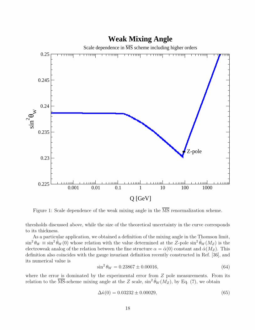
The resulting scale-dependence of sin2 θW (µ) for µ =√

|q2| with q2 being the four-momentumtransfer squared is shown in Fig. 1. The various discontinuities in the curve correspond to the

17

0.001 0.01 0.1 1 10 100 1000

Q [GeV]

0.225

0.23

0.235

0.24

0.245

0.25

sin2 θ W

Z-pole

Weak Mixing AngleScale dependence in MS scheme including higher orders

Figure 1: Scale dependence of the weak mixing angle in the MS renormalization scheme.

thresholds discussed above, while the size of the theoretical uncertainty in the curve correspondsto its thickness.

As a particular application, we obtained a definition of the mixing angle in the Thomson limit,sin2 θW ≡ sin2 θW (0) whose relation with the value determined at the Z-pole sin2 θW (MZ) is theelectroweak analog of the relation between the fine structure α = α(0) constant and α(MZ). Thisdefinition also coincides with the gauge invariant definition recently constructed in Ref. [36], andits numerical value is

sin2 θW = 0.23867 ± 0.00016, (64)

where the error is dominated by the experimental error from Z pole measurements. From itsrelation to the MS-scheme mixing angle at the Z scale, sin2 θW (MZ), by Eq. (7), we obtain

∆κ(0) = 0.03232 ± 0.00029, (65)

18

where now the error is purely theoretical. Finally, using the relation [48] between sin2 θW (MZ)and the effective leptonic mixing angle, sin2 θ eff

f , defined in Eq. (5), we obtain,

sin2 θW − sin2 θ effℓ = 0.00718 ± 0.00007. (66)

The error in this relation (which is the main result of this work) is an order of magnitude belowcurrent and anticipated experimental uncertainties and considerably smaller than the uncertaintyquoted in Refs. [15].

To illustrate the impact of this result on particular observables, we consider the weak chargeof the proton, QW (p), that will be determined using parity-violating elastic ep scattering atthe Jefferson Lab. Up-dating the recent analysis of Ref. [39], we obtain the Standard Modelprediction

QW (p) = 0.0713 ± 0.0006 (input) ± 0.0003 (∆κ) ± 0.0005 (Zγ box) ± 0.0001 (WW box)

= 0.0713 ± 0.0008, (67)

where the experimental uncertainties in sin2 θW (MZ) and mt (“input”), the theoretical hadronicuncertainties in ∆κ(0) and the Zγ box graph, and the uncertainty from unknown higher-orderperturbative QCD contributions to the WW box graphs are shown separately and combinedin quadrature in the second line. Use of the previous estimate for the uncertainty in ∆κ(0) of±0.0025 would lead to a theoretical (total) error in the QW (p) prediction roughly five (three)times larger than in Eq. (67), and in this case, one could neglect the uncertainties associated withother radiative corrections. In light of our analysis, however, the uncertainty in the StandardModel prediction is now three and a half times smaller than the anticipated experimental error,and theoretical uncertainties associated with hadronic contributions to other radiative correctionsbecome relatively more important.

In the same vein, the interpretation of the prospective parity violating deep inelastic measure-ments will require a careful analysis of higher twist and isospin breaking corrections, especiallygiven that the latter may be responsible for the present discrepancy between the NuTeV resultfor sin2 θW (µ ∼ 3 GeV) and the SM prediction. Our analysis applies to the deep inelastic regime,as well, where due to the higher energies involved, the uncertainty in sin2 θW (µ) is even muchsmaller since no complications from non-perturbative contributions arise in this case. Given thelevel of experimental effort required to carry out these precise low energy measurements, per-forming a theoretical analysis of these effects at the level we have attempted to do here for theweak mixing angle seems well-worth the effort.

Acknowledgments:

We are happy to thank Krishna Kumar, Paul Langacker, Philip Mannheim, Robert McKeown,Michael Pennington, Alberto Sirlin, and Peter Zerwas for very helpful discussions, and PeterZerwas also for a careful reading of the manuscript. We are grateful for the support from theInstitute for Nuclear Theory at the University of Washington, where this work was initiated. MR-M thanks the Physics Institute at UNAM for support and hospitality during a visit to undertake

19

this project. This work was supported in part by U.S. Department of Energy contracts DE–FG02–00ER41146, DE–FG03–02ER41215, and DE–FG03–00ER41132, by the National ScienceFoundation Award PHY00–71856, by CONACYT (Mexico) contract 42026–F, and by DGAPA–UNAM contract PAPIIT IN112902.

A Updated value for the mixing angle ǫ

Here we determine the phenomenological value of the ω-φ mixing angle, ǫ, defined by,

|ω〉 = cos ǫ|uu〉 + |dd〉√

2− sin ǫ|ss〉, |φ〉 = sin ǫ

|uu〉 + |dd〉√2

+ cos ǫ|ss〉, (68)

where ǫ = 0 is referred to as ideal mixing. One way to extract it is to use SU(3) flavor symmetryand first order breaking applied to the vector meson octet mass spectrum. An advantage ofthis method is that it can be calibrated against the ground state baryon octet, for which Fermistatistics precludes the mixing with an SU(3) singlet state. The mass of the SU(2) singlet, MΛ,is therefore predicted in terms of the masses of the other electrically neutral octet members,

MΛ =1

3(2Mn + 2MΞ0 − MΣ0) = 1105.4 MeV, (69)

which reproduces the experimental value [40], MΛ = 1115.7 MeV, within 0.93%. Analogously,the Gell-Mann-Okubo mass formula [41,42] yields the octet-octet component of the mass matrixfor the isosinglet ground state vector mesons,

M288 =

1

3(4M2

K∗0 − M2ρ0) = (933.69 MeV)2 × [1 ± 0.0008 ± 0.0020 ± 0.0121 ± 0.0093]. (70)

The first error is from the experimental uncertainty in the masses, which are taken from Ref. [40]except for the mass, Mρ0 = 775.74± 0.65 MeV, and the width, Γρ0 = 145.3± 1.4 MeV, of the ρ0

resonance for which we averaged Refs. [43,44]. The broadness of some of the resonances involvedintroduces an ambiguity as for what definition of mass one should use in the Gell-Mann-Okuboformula. For the central value we have chosen the peak position,

M =M

4

√

1 + Γ2

M2

, (71)

where M and Γ correspond to the usual definition of a relativistic Breit-Wigner resonance formwith an s-dependent width, i.e. the one used by the Particle Data Group [40]. The second errorin Eq. (70) reflects the size of the shift obtained by replacing M by M . The third error is due topossible isospin breaking effects which we estimated by using M2

K∗± in place of M2K∗0. The last

error quantifies the limitation of the method and is given by the calibration against the baryonoctet as discussed above. Adding all errors in quadrature, we obtain for the SU(3) octet-singletmixing angle [40], θV ,

tan2 θV =M2

88 − M2φ

M2ω − M2

88

= 0.646−0.081+0.090, (72)

20

which translates into the two solutions13, ǫ1 = 0.061 ∓ 0.032 and ǫ2 = −1.292 ± 0.032. Alterna-tively, one can compare the branching ratios of the ω and φ resonances decaying into π0γ [45],

tan2 ǫ =M3

φ

M3ω

(

M2ω − M2

π0

M2φ − M2

π0

)3 B(φ → π0γ)

B(ω → π0γ)

Γφ

Γω= (3.01 ± 0.26) × 10−3, (73)

which gives, |ǫ| = 0.0548±0.0024. Comparison with the previous method singles out the solution,

ǫ = +0.0548 ± 0.0024. (74)

The sign and magnitude are also consistent with various other methods [46] and the previousanalysis in Ref. [45].

B Phenomenological approach to OZI suppression

In Section 6 we argued that the OZI rule can at least partly be understood as a result ofgroup theoretical suppression factors relative to OZI allowed processes. Using the result ofAppendix A, we now wish to study OZI rule violating contributions to the mass matrix ofground state vector mesons. These mesons dominate the electromagnetic current correlatorat hadronic scales, and should therefore serve as a means to quantify OZI rule suppressionsphenomenologically. Throughout this Appendix we work in the isospin symmetric limit.

In the flavor basis, (|uu〉, |dd〉, |ss〉), we write the mass matrix in a form which is similar tothe one discussed in Ref. [47],

M =

A + B B B + CB A + B B + C

B + C B + C A + B + D

. (75)

The parameters A and B respect SU(3) symmetry, while C and D break it. The off-diagonal ele-ments, B and C, parametrize flavor transitions, and can only be generated by QCD annihilation(singlet) diagrams. The parameter D receives contributions from the strange quark mass, as wellas dynamical contributions of both singlet and non-singlet type. The difference to Ref. [47] isthat there C = 0, and B = B(µ) is a scale dependent singlet function, while we define all entriesof M as constants without specifying their relation to the scale dependent current correlators.In the isospin basis, (|(uu − dd)/

√2〉, |(uu + dd)/

√2〉, |ss〉), M reads,

M =

A 0 0

0 A + 2B√

2(B + C)

0√

2(B + C) A + B + D

, (76)

so that we can identify, A = M2ρ0 . The trace of M then yields the condition,

3B + D = M2ω + M2

φ − 2M2ρ0 , (77)

13Since Γφ ≪ Mφ and Γω ≪ Mω, the complex phase in ǫ can safely be neglected.

21

and ǫ obtained in Appendix A gives the constraint,

tan 2ǫ =√

8B + C

D − B. (78)

The final relation,

(M2φ − M2

ω)2 =[

3(B + C) − 1

3(C + D)

]2

+8

9(C + D)2, (79)

shows that in the SU(3) limit, C = D = 0, singlet diagrams associated with B would splitM2

φ from M2ρ0 = M2

ω in much the same way as triangle anomaly diagrams would split M2η′ from

M2η = M2

π . Taking into account that ǫ ≪ 1, we can approximate,

B ≈M2

ω − M2ρ0

2, D ≈ M2

φ −M2

ω + M2ρ0

2, (80)

which is correct up to O(ǫ2). Thus, in the limit of ideal mixing, B drives the splitting of M2ω

from M2ρ0 instead. In any case, the singlet contribution associated to B is very small compared

to A and D. More relevant for this work is the SU(3) breaking singlet parameter,

C ≈ M2φ − M2

ω√8

tan 2ǫ −M2

ω − M2ρ0

2, (81)

which reduces to C = −B in the ideal mixing case, ǫ = 0. Numerically, we have,

A = (769 MeV)2, B = (105 MeV)2,C = ( 74 MeV)2, D = (660 MeV)2.

(82)

There is a second solution in which |B|, |C|, and |D| are all comparable and where B ≈ −Cto ensure ǫ ≪ 1. It also has D < 0, although the strange quark mass is expected to givethe dominant (positive) contribution. Therefore we discard this solution. We can also roughlyestimate the singlet component contained in D by relating it to MK∗0,

Dsinglet ∼ D − 2(M2K∗0 − M2

ρ0) = (123 MeV)2, (83)

which is of similar size as B and C. Thus, singlet contributions to vector meson masses aregenerally suppressed by more than an order of magnitude beyond the QCD suppression factorsdiscussed in Section 6 indicating that the smallness of the known coefficient, C2 ≪ 1, may indeedbe a generic feature that persists at higher orders. Qualitatively the same results are obtainedif linear mass relations are used in place of masses squared, except that singlet contributionsappear even more suppressed.

References

[1] M. J. G. Veltman, Nucl. Phys. B 123, 89 (1977).

22

[2] W. A. Bardeen, A. J. Buras, D. W. Duke and T. Muta, Phys. Rev. D 18, 3998 (1978).

[3] S. Weinberg, Phys. Lett. B 91, 51 (1980).

[4] W. J. Marciano and A. Sirlin, Phys. Rev. Lett. 46, 163 (1981).

[5] W. J. Marciano and J. L. Rosner, Phys. Rev. Lett. 65, 2963 (1990) and Erratum ibid. 68,898 (1992).

[6] S. Fanchiotti, B. A. Kniehl and A. Sirlin, Phys. Rev. D 48, 307 (1993).

[7] C. S. Wood et al., Science 275, 1759 (1997).

[8] SLAC–E–158 Collaboration: P. L. Anthony et al., Phys. Rev. Lett. 92, 181602 (2004) andhep-ex/0504049.

[9] Qweak Collaboration: D. S. Armstrong et al., AIP Conf. Proc. 698, 172 (2004).

[10] A. Czarnecki and W. J. Marciano, Phys. Rev. D 53, 1066 (1996).

[11] A. Czarnecki and W. J. Marciano, Int. J. Mod. Phys. A 15, 2365 (2000).

[12] M. J. Musolf and B. R. Holstein, Phys. Lett. B 242, 461 (1990).

[13] M. J. Musolf and B. R. Holstein, Phys. Rev. D 43, 2956 (1991).

[14] W. J. Marciano and A. Sirlin, Phys. Rev. D 22, 2695 (1980) and Erratum ibid. 31, 213(1985).

[15] W. J. Marciano, Radiative Corrections to Neutral Current Processes, p. 170 in Ref. [35].

[16] NuTeV Collaboration: G. P. Zeller et al., Phys. Rev. Lett. 88, 091802 (2002) and Erratumibid. 90, 239902 (2003).

[17] S. G. Gorishnii, A. L. Kataev and S. A. Larin, Phys. Lett. B 212, 238 (1988) and ibid. 259,144 (1991).

[18] L. R. Surguladze and M. A. Samuel, Phys. Rev. Lett. 66, 560 (1991) and Erratum ibid. 66,2416 (1991).

[19] S. A. Larin, T. van Ritbergen and J. A. M. Vermaseren, Nucl. Phys. B 438, 278 (1995).

[20] K. G. Chetyrkin, J. H. Kuhn and M. Steinhauser, Nucl. Phys. B 482, 213 (1996).

[21] J. Erler, Phys. Rev. D 59, 054008 (1999).

[22] L. J. Hall, Nucl. Phys. B 178, 75 (1981).

[23] I. Antoniadis, C. Kounnas and K. Tamvakis, Phys. Lett. B 119, 377 (1982).

23

[24] P. Langacker and N. Polonsky, Phys. Rev. D 47, 4028 (1993).

[25] F. Jegerlehner, Renormalizing the Standard Model, p. 476 in Ref. [26].

[26] M. Cvetic and P. Langacker, Testing the Standard Model, Proceedings of the TheoreticalAdvanced Study Institute in Elementary Particle Physics, Boulder, USA, June 3–27 (1990).

[27] M. Davier and A. Hocker, Phys. Lett. B 435, 427 (1998).

[28] M. Davier, S. Eidelman, A. Hocker and Z. Zhang, Eur. Phys. J. C 31, 503 (2003).

[29] B. A. Kniehl, Phys. Lett. B 237, 127 (1990).

[30] A. H. Hoang, M. Jezabek, J. H. Kuhn and T. Teubner, Phys. Lett. B 338, 330 (1994).

[31] S. Okubo, Phys. Lett. 5, 165 (1963).

[32] G. Zweig, An SU(3) Model For Strong Interaction Symmetry And Its Breaking, 2, CERNReport No. 8419/TH 412 (1964).

[33] J. Iizuka, Prog. Theor. Phys. Suppl. 37, 21 (1966).

[34] T. van Ritbergen, A. N. Schellekens and J. A. M. Vermaseren, Int. J. Mod. Phys. A 14, 41(1999).

[35] P. Langacker, Precision Tests of the Standard Electroweak Model, Advanced series on di-rections in high energy physics: 14 (World Scientific, Singapore, Singapore, 1995).

[36] A. Ferroglia, G. Ossola and A. Sirlin, Eur. Phys. J. C 34, 165 (2004).

[37] G. Degrassi and A. Sirlin, Phys. Rev. D 46, 3104 (1992).

[38] D. R. T. Jones, Phys. Rev. D 25, 581 (1982).

[39] J. Erler, A. Kurylov and M. J. Ramsey-Musolf, Phys. Rev. D 68, 016006 (2003).

[40] Particle Data Group: S. Eidelman et al., Phys. Lett. B 592, 1 (2004).

[41] S. Okubo, Prog. Theor. Phys. 27, 949 (1962).

[42] M. Gell-Mann, Phys. Rev. 125, 1067 (1962).

[43] L. M. Barkov et al., Nucl. Phys. B 256, 365 (1985).

[44] CMD-2 Collaboration: R. R. Akhmetshin et al., Phys. Lett. B 578, 285 (2004).

[45] P. Jain et al., Phys. Rev. D 37, 3252 (1988).

[46] J. Arafune, M. Fukugita and Y. Oyanagi, Phys. Lett. B 70, 221 (1977).

[47] A. De Rujula, H. Georgi and S. L. Glashow, Phys. Rev. D 12, 147 (1975).

[48] P. Gambino and A. Sirlin, Phys. Rev. D 49, 1160 (1994).

24