Fabrication of paper-based enzyme immobilized microarray ...
Upload
vprasarnth-raajCategory
view
2.685download
419description
BK10110302 V.PRASARNTH RAAJ VEERA RAO – BIOPROCESS
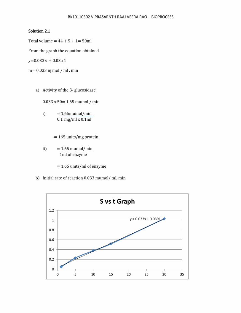
y = 0.033x + 0.0391
0
0.2
0.4
0.6
0.8
1
1.2
0 5 10 15 20 25 30 35
S vs t Graph
Solution 2.1
Total volume = 44 + 5 + 1= 50ml
From the graph the equation obtained
y=0.033× + 0.03a 1
m= 0.033 ɱ mol / ml . min
a) Activity of the β- glucosidase
0.033 x 50= 1.65 mumol / min
i) = 1.65mumol/min
0.1 mg/ml x 0.1ml
= 165 units/mg protein
ii) = 1.65 mumol/min
1ml of enzyme
= 1.65 units/ml of enzyme
b) Initial rate of reaction 0.033 mumol/ mL.min
BK10110302 V.PRASARNTH RAAJ VEERA RAO – BIOPROCESS
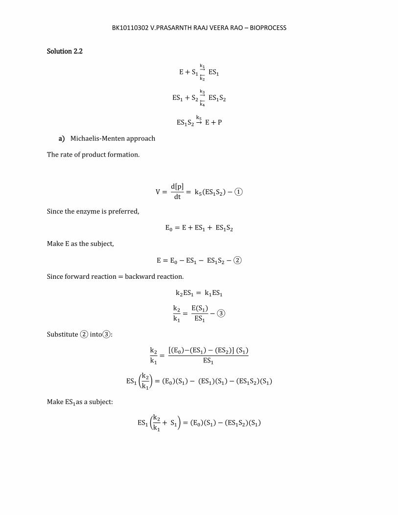
Solution 2.2
←
→
←
→
→
a) Michaelis-Menten approach
The rate of product formation.
d[p]
dt ( )
Since the enzyme is preferred,
Make E as the subject,
Since forward reaction = backward reaction.
( )
ubstitute into :
[( ) ( ) ( )] ( )
( ) ( )( ) ( )( ) ( )( )
Make as a subject:
( ) ( )( ) ( )( )

BK10110302 V.PRASARNTH RAAJ VEERA RAO – BIOPROCESS
( )( ) ( )( )
( )
( ) [( )( )]
( )( )
( )
( ) ( )( )
ub into :
( ) ( )( ) ( )( )
( ) ( )( )( ) ( )( )( )
Make as a subject,
( )( ( )( ))
( )( )( )
( ) ( )( )( )
( )(
( )( ))
( ) ( )( )( )
(
) ( ) ( )( )
ub into ,
BK10110302 V.PRASARNTH RAAJ VEERA RAO – BIOPROCESS
d[p]
dt (
( )( )( )
( ) ( )( )
)
( )( )( )
( ) ( )( )
)
Since ( )
( )( )
( ) ( )( )
)
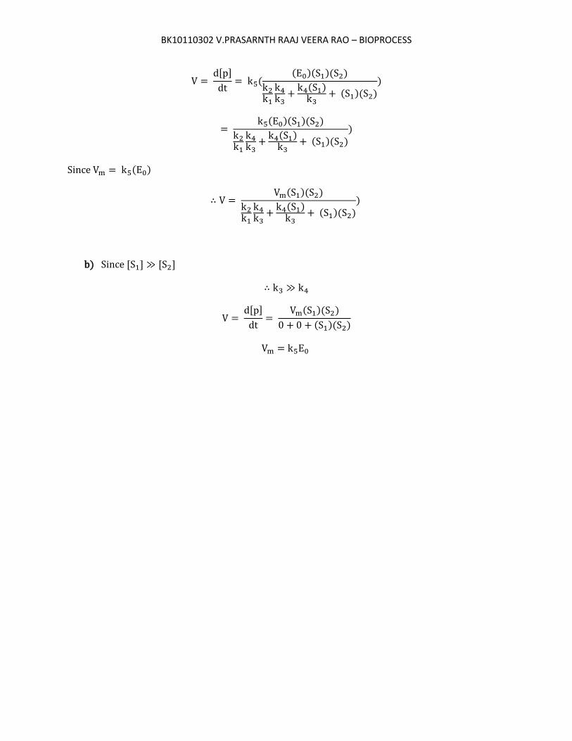
b) Since [ ] [ ]
d[p]
dt ( )( )
( )( )
BK10110302 V.PRASARNTH RAAJ VEERA RAO – BIOPROCESS
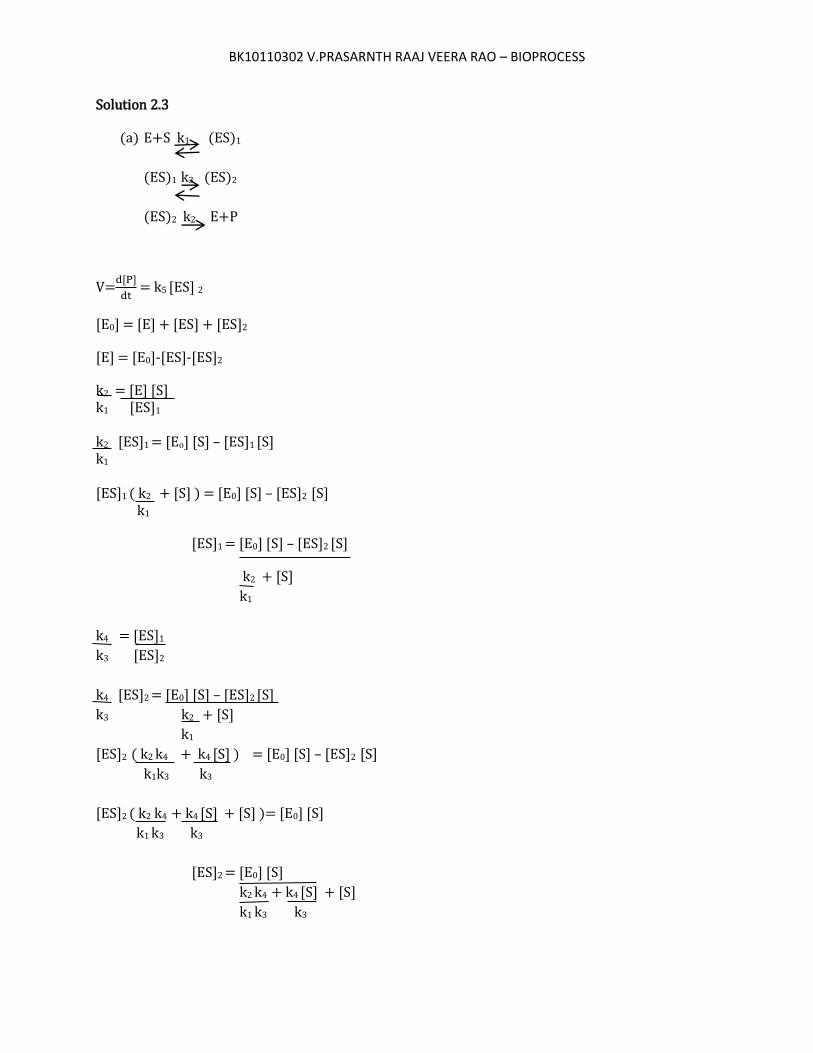
Solution 2.3
(a) E+S k1 (ES)1
(ES)1 k3 (ES)2
(ES)2 k2 E+P
V= [ ]
= k5 [ES] 2
[E0] = [E] + [ES] + [ES]2
[E] = [E0]-[ES]-[ES]2
k2 = [E] [S] k1 [ES]1
k2 [ES]1 = [Eo] [S] – [ES]1 [S] k1
[ES]1 ( k2 + [S] ) = [E0] [S] – [ES]2 [S]
k1
[ES]1 = [E0] [S] – [ES]2 [S]
k2 + [S]
k1
k4 = [ES]1
k3 [ES]2
k4 [ES]2 = [E0] [S] – [ES]2 [S]
k3 k2 + [S]
k1
[ES]2 ( k2 k4 + k4 [S] ) = [E0] [S] – [ES]2 [S]
k1k3 k3
[ES]2 ( k2 k4 + k4 [S] + [S] )= [E0] [S]
k1 k3 k3
[ES]2 = [E0] [S]
k2 k4 + k4 [S] + [S]
k1 k3 k3
BK10110302 V.PRASARNTH RAAJ VEERA RAO – BIOPROCESS
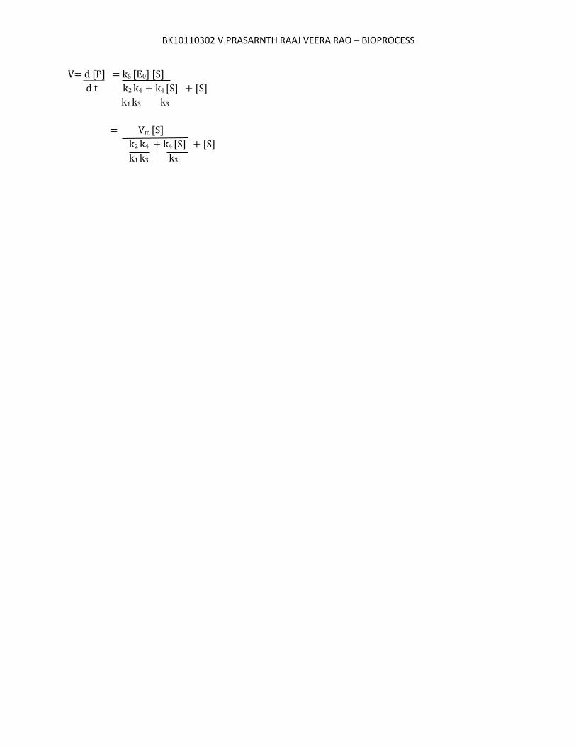
V= d [P] = k5 [E0] [S]
d t k2 k4 + k4 [S] + [S]
k1 k3 k3
= Vm [S]
k2 k4 + k4 [S] + [S]
k1 k3 k3
BK10110302 V.PRASARNTH RAAJ VEERA RAO – BIOPROCESS
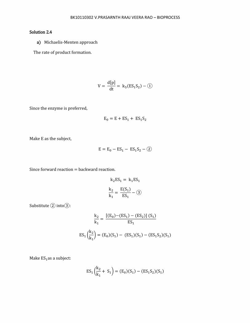
Solution 2.4
a) Michaelis-Menten approach
The rate of product formation.
d[p]
dt ( )
Since the enzyme is preferred,
Make E as the subject,
Since forward reaction = backward reaction.
( )
ubstitute into :
[( ) ( ) ( )] ( )
( ) ( )( ) ( )( ) ( )( )
Make as a subject:
( ) ( )( ) ( )( )
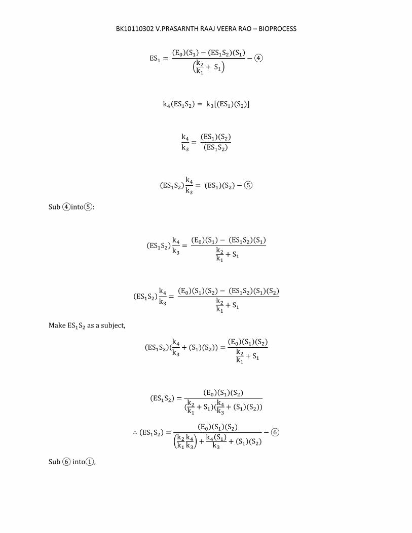
BK10110302 V.PRASARNTH RAAJ VEERA RAO – BIOPROCESS
( )( ) ( )( )
( )
( ) [( )( )]
( )( )
( )
( ) ( )( )
ub into :
( ) ( )( ) ( )( )
( ) ( )( )( ) ( )( )( )
Make as a subject,
( )( ( )( ))
( )( )( )
( ) ( )( )( )
( )(
( )( ))
( ) ( )( )( )
(
) ( ) ( )( )
ub into ,
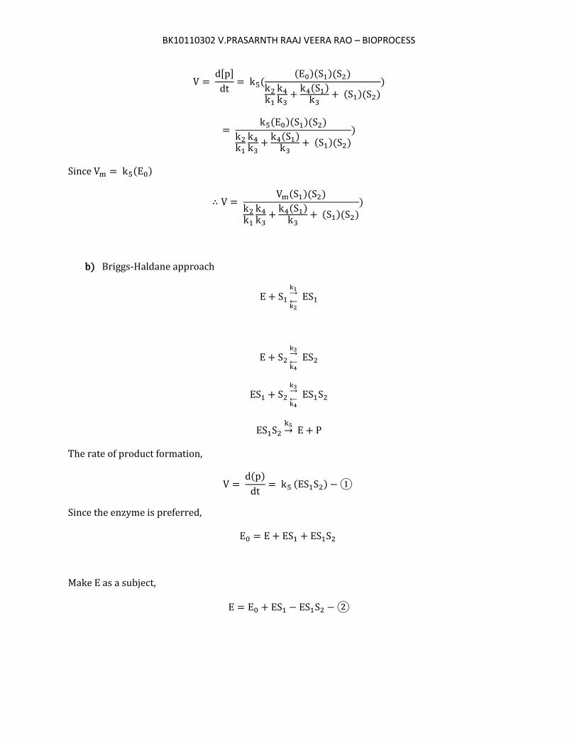
BK10110302 V.PRASARNTH RAAJ VEERA RAO – BIOPROCESS
d[p]
dt (
( )( )( )
( ) ( )( )
)
( )( )( )
( ) ( )( )
)
Since ( )
( )( )
( ) ( )( )
)
b) Briggs-Haldane approach
←
→
←
→
←
→
→
The rate of product formation,
d(p)
dt ( )
Since the enzyme is preferred,
Make as a subject,
BK10110302 V.PRASARNTH RAAJ VEERA RAO – BIOPROCESS
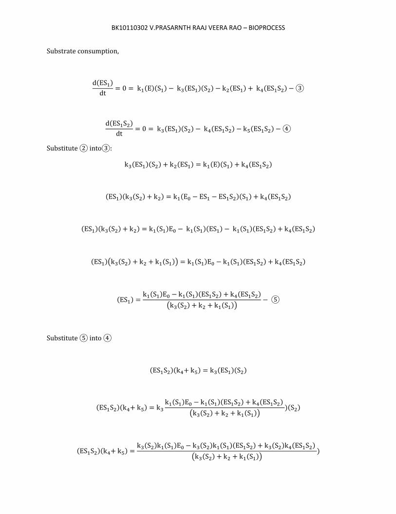
Substrate consumption,
d( )
dt ( )( ) ( )( ) ( ) ( )
d( )
dt ( )( ) ( ) ( )
ubstitute into :
( )( ) ( ) ( )( ) ( )
( )( ( ) ) ( )( ) ( )
( )( ( ) ) ( ) ( )( ) ( )( ) ( )
( )( ( ) ( )) ( ) ( )( ) ( )
( ) ( ) ( )( ) ( )
( ( ) ( ))
ubstitute into
( )( ) ( )( )
( )( ) ( ) ( )( ) ( )
( ( ) ( )))( )
( )( ) ( ) ( ) ( ) ( )( ) ( ) ( )
( ( ) ( )))

BK10110302 V.PRASARNTH RAAJ VEERA RAO – BIOPROCESS
( )( )( ( ) ( ))
( ) ( ) ( ) ( )( ) ( ) ( )
( )( ( ) ( ) ( ) )( ( ) ( )) ( ) ( )
( ) ( ) ( )
( ( ) ( ) ( ) )( ( ) ( ))
ubstitute into
d(p)
dt (
( ) ( )
( ( ) ( ) ( ) )( ( ) ( ))
v
d(p)
dt
v ( ) ( )
( ( ) ( ) ( ) )( ( ) ( ))
BK10110302 V.PRASARNTH RAAJ VEERA RAO – BIOPROCESS
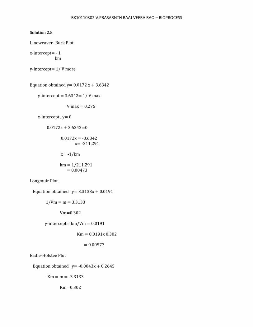
Solution 2.5
Lineweaver- Burk Plot
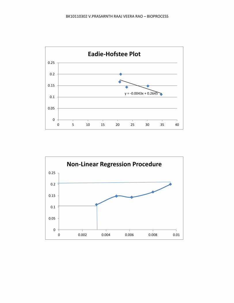
x-intercept= - 1 km y-intercept= 1/ V more Equation obtained y= 0.0172 x + 3.6342 y-intercept = 3.6342= 1/ V max V max = 0.275 x-intercept , y= 0 0.0172x + 3.6342=0 0.0172x = -3.6342 x= -211.291 x= -1/km km = 1/211.291 = 0.00473 Longmuir Plot Equation obtained y= 3.3133x + 0.0191 1/Vm = m = 3.3133 Vm=0.302 y-intercept= km/Vm = 0.0191 Km = 0,0191x 0.302 = 0.00577 Eadie-Hofstee Plot Equation obtained y= -0.0043x + 0.2645 -Km = m = -3.3133 Km=0.302
BK10110302 V.PRASARNTH RAAJ VEERA RAO – BIOPROCESS
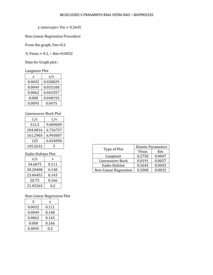
y-intercept= Vm = 0.2645 Non-Linear Regression Procedure
From the graph, Vm=0.2
½ Vmax = 0.1, Km=0.0032
Data for Graph plot :
Langmuir Plot
s s/v
0.0032 0.028829
0.0049 0.033108
0.0062 0.043357
0.008 0.048193
0.0095 0.0475
Lineweaver-Burk Plot
Eadie-Hofstee Plot
v/s v
34.6875 0.111
30.20408 0.148
23.06452 0.143
20.75 0.166
21.05263 0.2
Non-Linear Regression Plot
S v
0.0032 0.111
0.0049 0.148
0.0062 0.143
0.008 0.166
0.0095 0.2
Type of Plot Kinetic Parameters
Vmax Km Langmuir 0.2750 0.0047
Lineweaver-Burk 0.0191 0.0057 Eadie-Hofstee 0.2645 0.0043
Non-Linear Regression 0.2000 0.0032
1/s 1/v
312.5 9.009009
204.0816 6.756757
161.2903 6.993007
125 6.024096
105.2632 5
BK10110302 V.PRASARNTH RAAJ VEERA RAO – BIOPROCESS
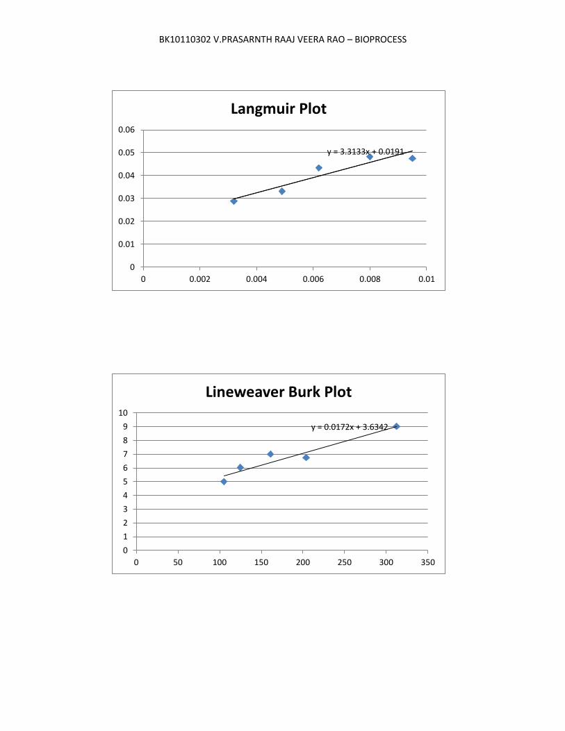
y = 3.3133x + 0.0191
0
0.01
0.02
0.03
0.04
0.05
0.06
0 0.002 0.004 0.006 0.008 0.01
Langmuir Plot
y = 0.0172x + 3.6342
0
1
2
3
4
5
6
7
8
9
10
0 50 100 150 200 250 300 350
Lineweaver Burk Plot
BK10110302 V.PRASARNTH RAAJ VEERA RAO – BIOPROCESS
y = -0.0043x + 0.2645
0
0.05
0.1
0.15
0.2
0.25
0 5 10 15 20 25 30 35 40
Eadie-Hofstee Plot
0
0.05
0.1
0.15
0.2
0.25
0 0.002 0.004 0.006 0.008 0.01
Non-Linear Regression Procedure
BK10110302 V.PRASARNTH RAAJ VEERA RAO – BIOPROCESS
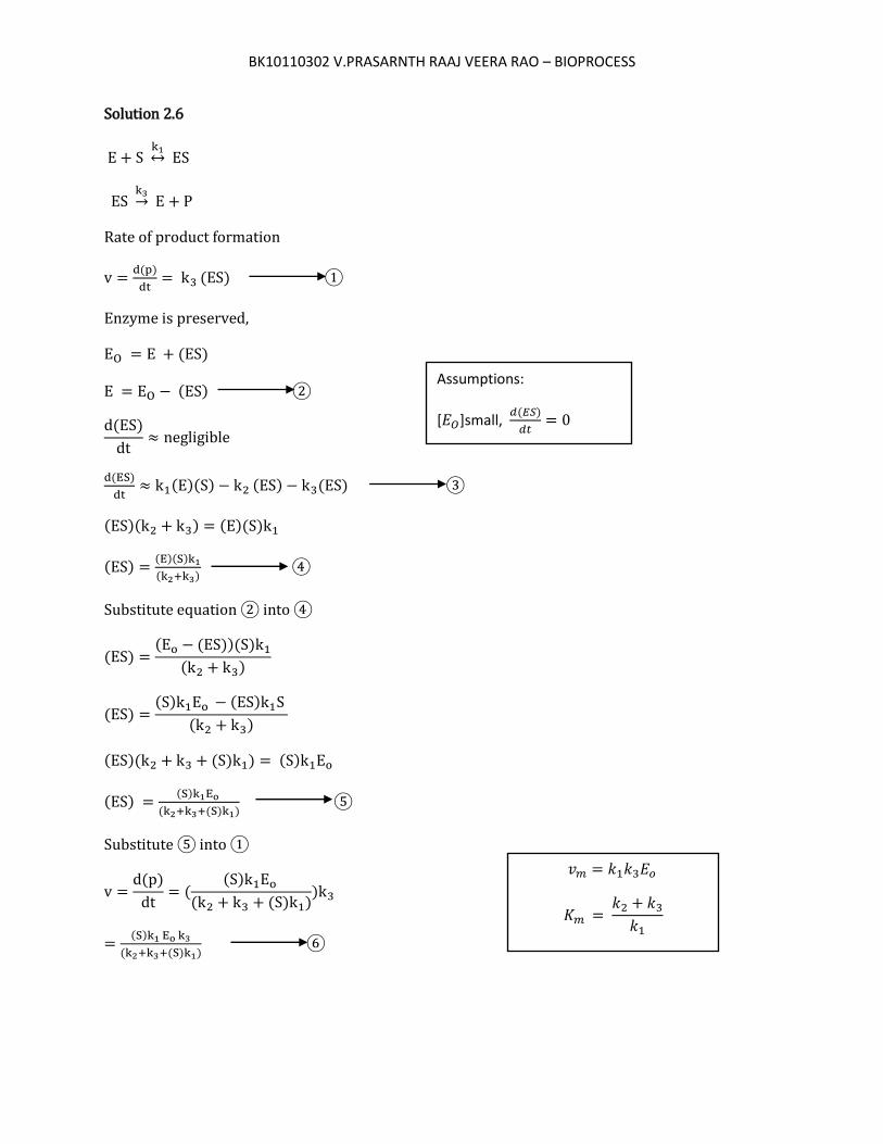
Solution 2.6
↔
→
Rate of product formation
v ( )
( )
Enzyme is preserved,
( )
( )
d( )
dt neg igib e
( )
( )( ) ( ) ( )
( )( ) ( )( )
( ) ( )( ) ( )
Substitute equation into
( ) ( ( ))( ) ( )
( ) ( ) ( )
( )
( )( ( ) ) ( )
( ) ( )
( ( ) )
Substitute into
v d(p)
dt (
( ) ( ( ) )
)
( )
( ( ) )
Assumptions:
[𝐸𝑂]small, 𝑑(𝐸𝑆)
𝑑𝑡
𝑣𝑚 𝑘 𝑘 𝐸𝑜
𝐾𝑚 𝑘 𝑘 𝑘
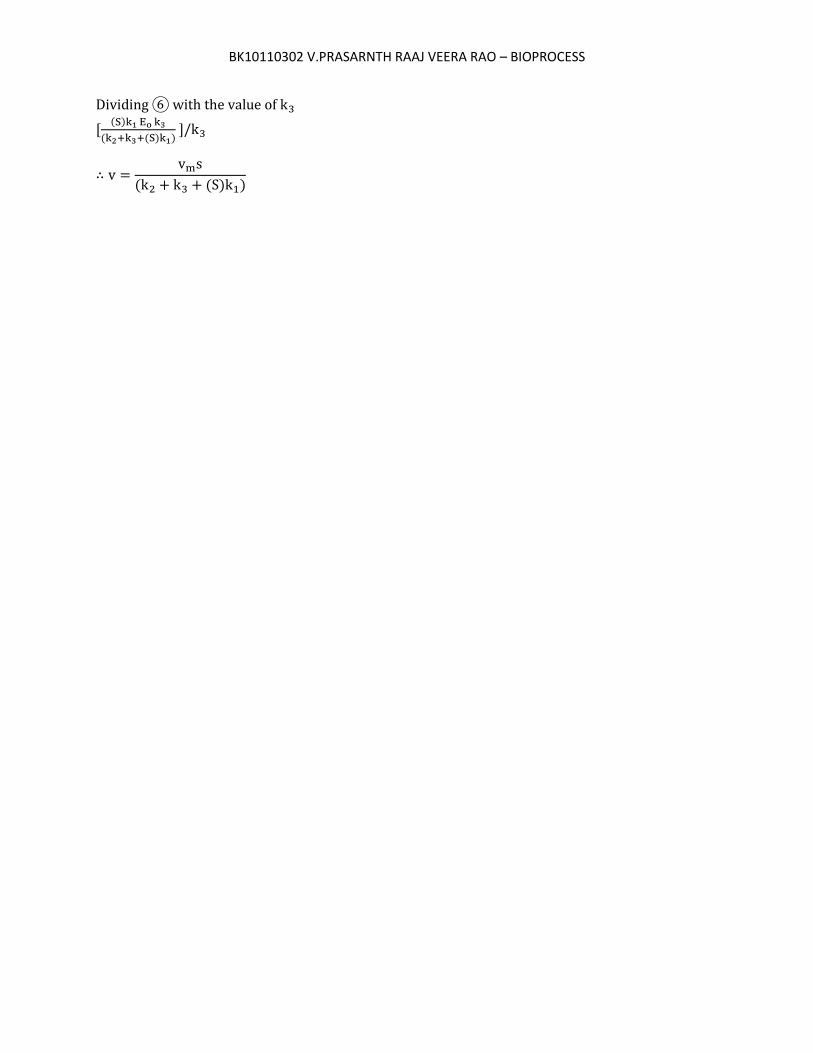
BK10110302 V.PRASARNTH RAAJ VEERA RAO – BIOPROCESS
Dividing with the value of
[( )
( ( ) ) ]/
v v s
( ( ) )
BK10110302 V.PRASARNTH RAAJ VEERA RAO – BIOPROCESS
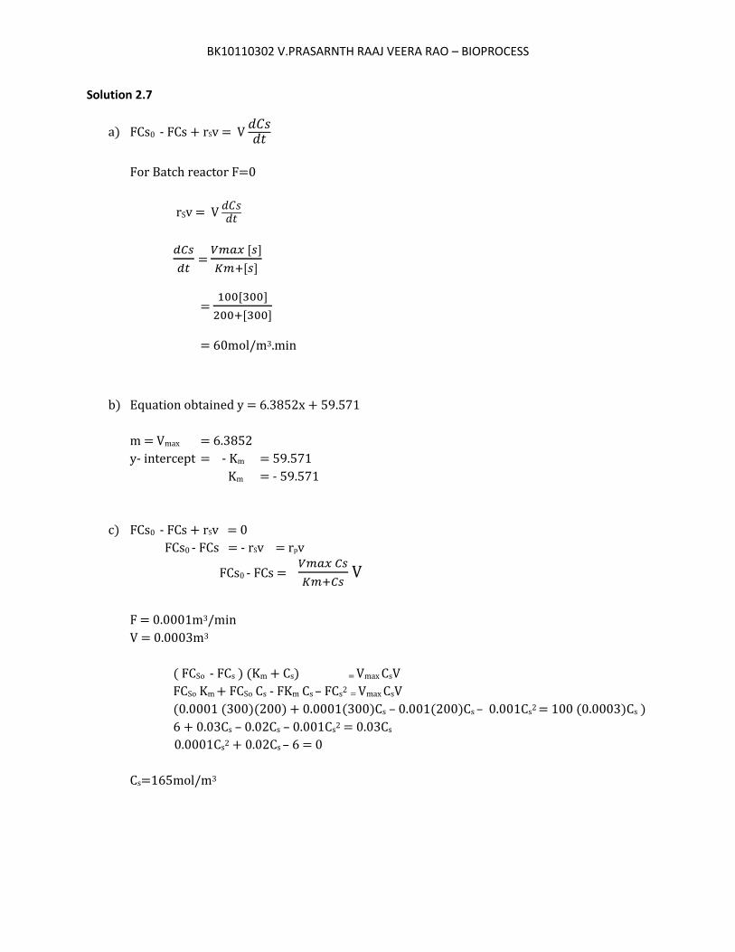
Solution 2.7
a) FCs0 - FCs + rSv = V
For Batch reactor F=0
rSv = V
= [ ]
[ ]
= [ ]
[ ]
= 60mol/m3.min
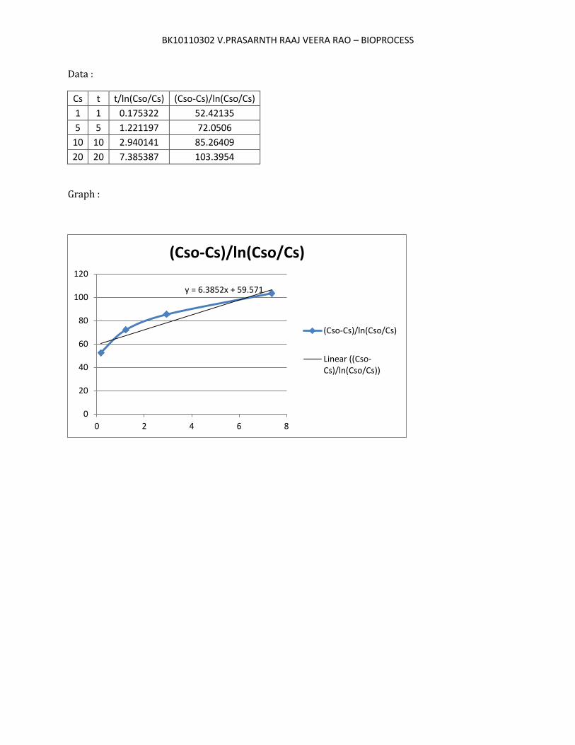
b) Equation obtained y = 6.3852x + 59.571
m = Vmax = 6.3852
y- intercept = - Km = 59.571
Km = - 59.571
c) FCs0 - FCs + rSv = 0
FCs0 - FCs = - rSv = rpv
FCs0 - FCs =
V
F = 0.0001m3/min
V = 0.0003m3
( FCSo - FCs ) (Km + Cs) = Vmax CsV
FCSo Km + FCSo Cs - FKm Cs – FCs2 = Vmax CsV
(0.0001 (300)(200) + 0.0001(300)Cs – 0.001(200)Cs – 0.001Cs2 = 100 (0.0003)Cs )
6 + 0.03Cs – 0.02Cs – 0.001Cs2 = 0.03Cs
0.0001Cs2 + 0.02Cs – 6 = 0
Cs=165mol/m3
BK10110302 V.PRASARNTH RAAJ VEERA RAO – BIOPROCESS
Data :
Cs t t/ln(Cso/Cs) (Cso-Cs)/ln(Cso/Cs)
1 1 0.175322 52.42135
5 5 1.221197 72.0506
10 10 2.940141 85.26409
20 20 7.385387 103.3954
Graph :
y = 6.3852x + 59.571
0
20
40
60
80
100
120
0 2 4 6 8
(Cso-Cs)/ln(Cso/Cs)
(Cso-Cs)/ln(Cso/Cs)
Linear ((Cso-Cs)/ln(Cso/Cs))
BK10110302 V.PRASARNTH RAAJ VEERA RAO – BIOPROCESS
Solution 2.8
a) Km =0.01 mol/L Cso = 3.4 x 10 -4 mol/L Cs = 0.9 x 3.4 x 10-4
= 3.06 x 10⁻⁴ mol/L t= 5minutes
= [ ]
[ ]
( 3.4x 10⁻⁴ – 3.06 x 10⁻⁴) = Vmax (3.06 x 10⁻⁴) S 0.01 + (3.06 x 10⁻⁴) 6.8 x 10-6 = Vmax ( 0.03) Vmax = 2.27 x 10⁻⁴ mol/L-min
b) 6.8 x 10-6 x 15 = 1.02 x 10⁻⁴ mol/L
BK10110302 V.PRASARNTH RAAJ VEERA RAO – BIOPROCESS
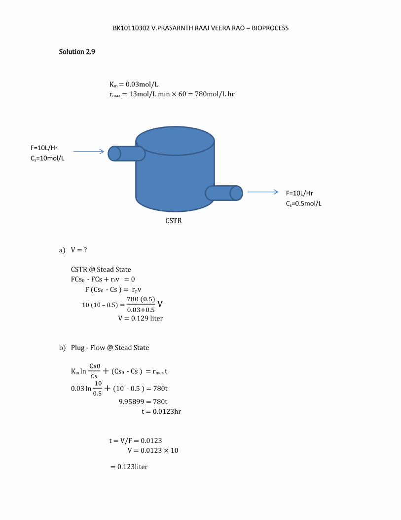
Solution 2.9
Km = 0.03mol/L
rmax = 13mol/L min × 60 = 780mol/L hr
CSTR
a) V = ?
CSTR @ Stead State
FCs0 - FCs + rSv = 0
F (Cs0 - Cs ) = rpv
10 (10 – 0.5) = ( )
V
V = 0.129 liter
b) Plug - Flow @ Stead State
Km ln
+ (Cs0 - Cs ) = rmax t
0.03 ln
+ (10 - 0.5 ) = 780t
9.95899 = 780t
t = 0.0123hr
t = V/F = 0.0123
V = 0.0123 × 10
= 0.123liter
F=10L/Hr
Cs=0.5mol/L
F=10L/Hr
Cs=10mol/L
BK10110302 V.PRASARNTH RAAJ VEERA RAO – BIOPROCESS
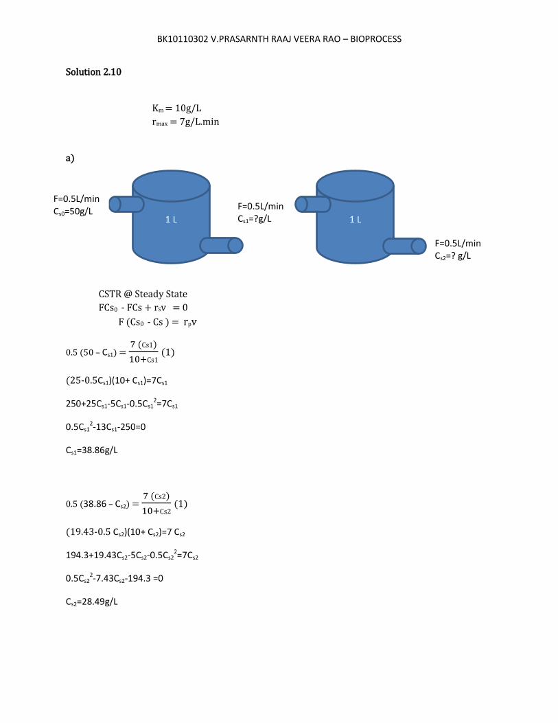
Solution 2.10
Km = 10g/L
rmax = 7g/L.min
a)
CSTR @ Steady State
FCs0 - FCs + rSv = 0
F (Cs0 - Cs ) = rpv
0.5 (50 – Cs1) = ( s )
s (1)
(25-0.5Cs1)(10+ Cs1)=7Cs1
250+25Cs1-5Cs1-0.5Cs12=7Cs1
0.5Cs12-13Cs1-250=0
Cs1=38.86g/L
0.5 (38.86 – Cs2) = ( s )
s (1)
(19.43-0.5 Cs2)(10+ Cs2)=7 Cs2
194.3+19.43Cs2-5Cs2-0.5Cs22=7Cs2
0.5Cs22-7.43Cs2-194.3 =0
Cs2=28.49g/L
1 L 1 L
F=0.5L/min Cs0=50g/L
F=0.5L/min Cs2=? g/L
F=0.5L/min Cs1=?g/L
BK10110302 V.PRASARNTH RAAJ VEERA RAO – BIOPROCESS
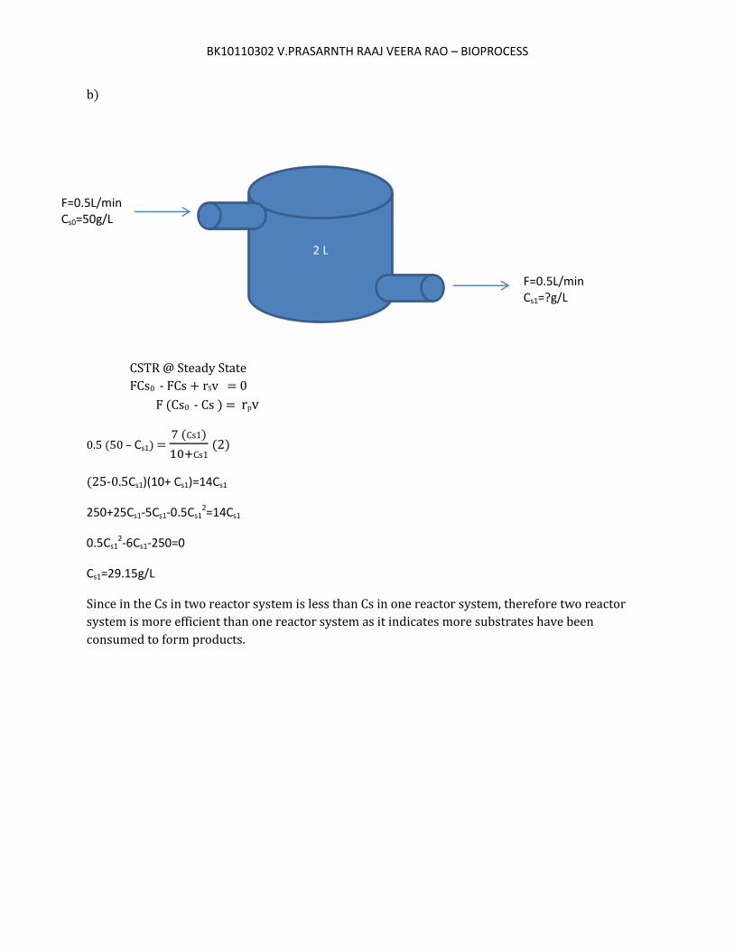
b)
CSTR @ Steady State
FCs0 - FCs + rSv = 0
F (Cs0 - Cs ) = rpv
0.5 (50 – Cs1) = ( s )
s (2)
(25-0.5Cs1)(10+ Cs1)=14Cs1
250+25Cs1-5Cs1-0.5Cs12=14Cs1
0.5Cs12-6Cs1-250=0
Cs1=29.15g/L
Since in the Cs in two reactor system is less than Cs in one reactor system, therefore two reactor
system is more efficient than one reactor system as it indicates more substrates have been
consumed to form products.
2 L
F=0.5L/min Cs0=50g/L
F=0.5L/min Cs1=?g/L
BK10110302 V.PRASARNTH RAAJ VEERA RAO – BIOPROCESS
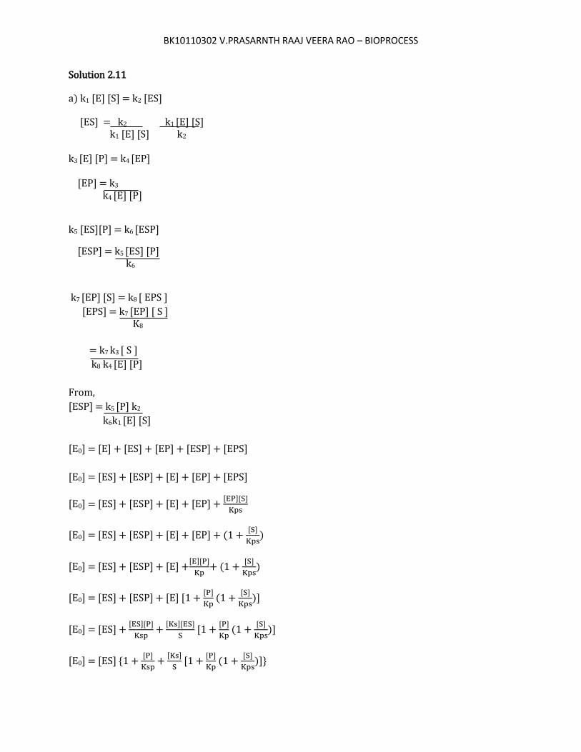
Solution 2.11
a) k1 [E] [S] = k2 [ES]
[ES] = k2 k1 [E] [S] k1 [E] [S] k2
k3 [E] [P] = k4 [EP] [EP] = k3
k4 [E] [P]
k5 [ES][P] = k6 [ESP]
[ESP] = k5 [ES] [P] k6
k7 [EP] [S] = k8 [ EPS ]
[EPS] = k7 [EP] [ S ] K8
= k7 k3 [ S ]
k8 k4 [E] [P]
From,
[ESP] = k5 [P] k2
k6k1 [E] [S]
[E0] = [E] + [ES] + [EP] + [ESP] + [EPS]
[E0] = [ES] + [ESP] + [E] + [EP] + [EPS]
[E0] = [ES] + [ESP] + [E] + [EP] + [ ][ ]
[E0] = [ES] + [ESP] + [E] + [EP] + ( [ ]
)
[E0] = [ES] + [ESP] + [E] +[ ][ ]
+ (
[ ]
)
[E0] = [ES] + [ESP] + [E] [ [ ]
(
[ ]
)]
[E0] = [ES] + [ ][ ]
+ [ ][ ]
[
[ ]
(
[ ]
)]
[E0] = [ES] {1 + [ ]
+ [ ]
[
[ ]
(
[ ]
)]}
BK10110302 V.PRASARNTH RAAJ VEERA RAO – BIOPROCESS
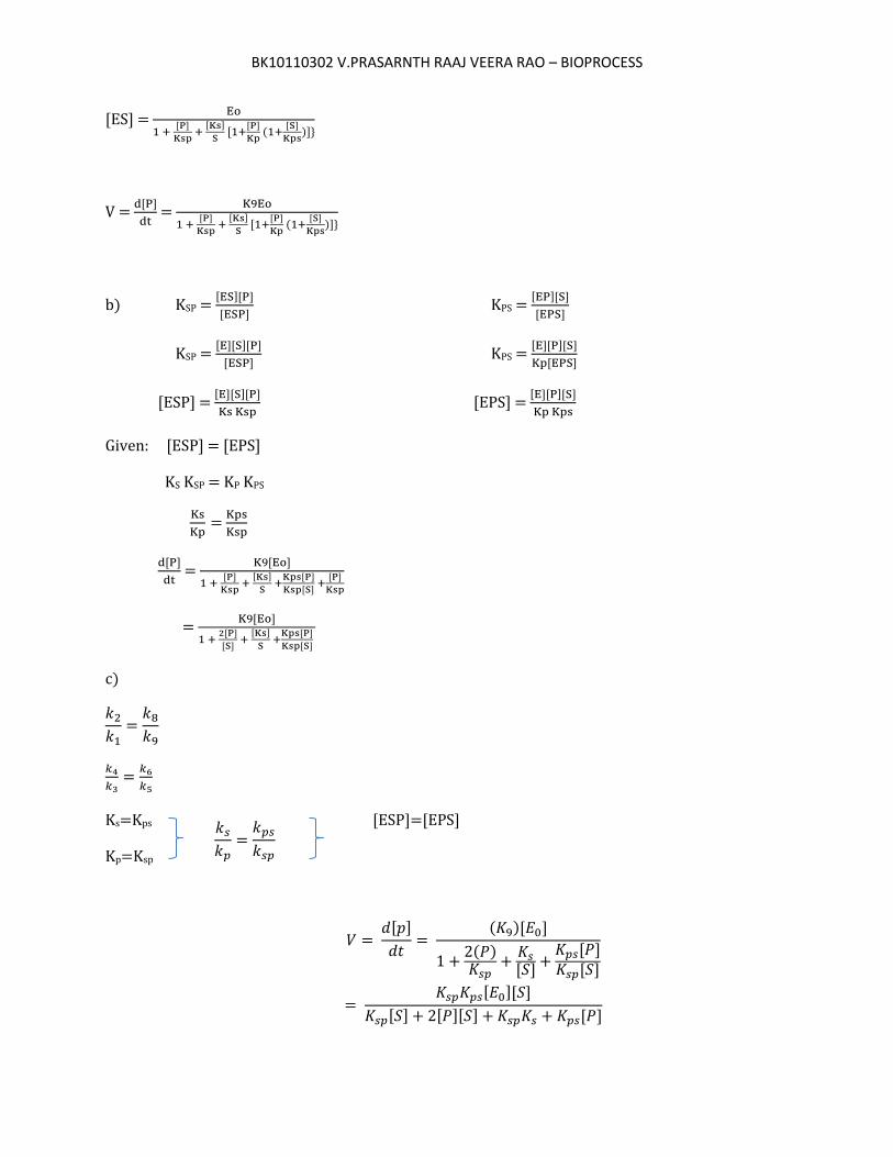
[ES] =
[ ]
[ ]
[ [ ]
(
[ ]
)]
V = [ ]
=
[ ]
[ ]
[ [ ]
(
[ ]
)]
b) KSP = [ ][ ]
[ ] KPS =
[ ][ ]
[ ]
KSP = [ ][ ][ ]
[ ] KPS =
[ ][ ][ ]
[ ]
[ESP] = [ ][ ][ ]
[EPS] =
[ ][ ][ ]
Given: [ESP] = [EPS]
KS KSP = KP KPS
=
[ ]
=
[ ]
[ ]
[ ]
[ ]
[ ] [ ]
= [ ]
[ ]
[ ] [ ]
[ ]
[ ]
c)
Ks=Kps [ESP]=[EPS]
Kp=Ksp
[ ]
( )[ ]
( ) [ ] [ ] [ ]
[ ][ ]
[ ] [ ][ ] [ ]
𝑘𝑠𝑘𝑝 𝑘𝑝𝑠𝑘𝑠𝑝
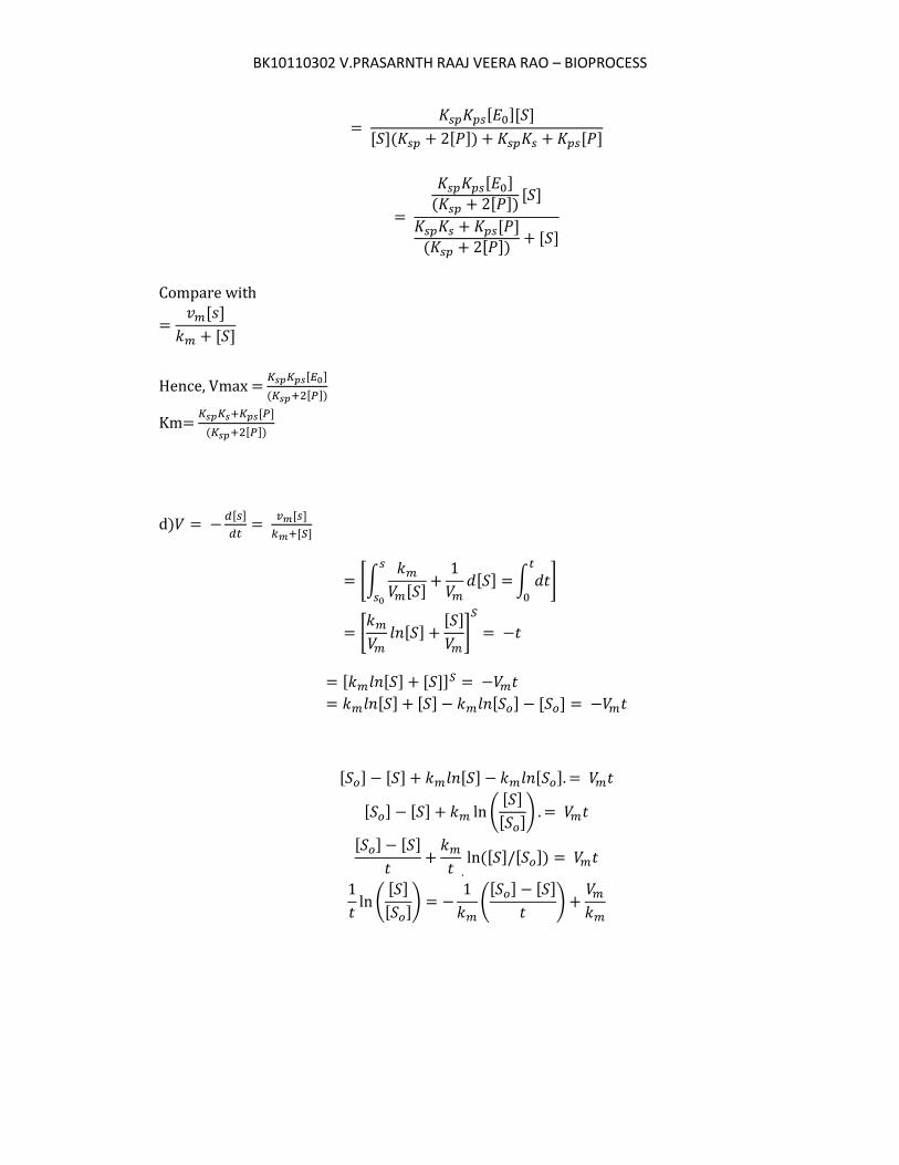
BK10110302 V.PRASARNTH RAAJ VEERA RAO – BIOPROCESS
[ ][ ]
[ ]( [ ]) [ ]
[ ]
( [ ])[ ]
[ ]
( [ ]) [ ]
Compare with
[ ]
[ ]
Hence, Vmax = [ ]
( [ ])
Km= [ ]
( [ ])
d) [ ]
[ ]
[ ]
*∫ [ ]
[ ]
∫
+
* [ ]
[ ]
+
[ [ ] [ ]]
[ ] [ ] [ ] [ ]
[ ] [ ] [ ] [ ]
[ ] [ ] n ([ ]
[ ])
[ ] [ ]
n ([ ] [ ])
n ([ ]
[ ])
([ ] [ ]
)
BK10110302 V.PRASARNTH RAAJ VEERA RAO – BIOPROCESS
Y = mx+c
Y =
n ([ ]
[ ])
M=
X= ([ ] [ ]
)
C=
So we can plot a graph of
n ([ ]
[ ]) vs (
[ ] [ ]
)
BK10110302 V.PRASARNTH RAAJ VEERA RAO – BIOPROCESS
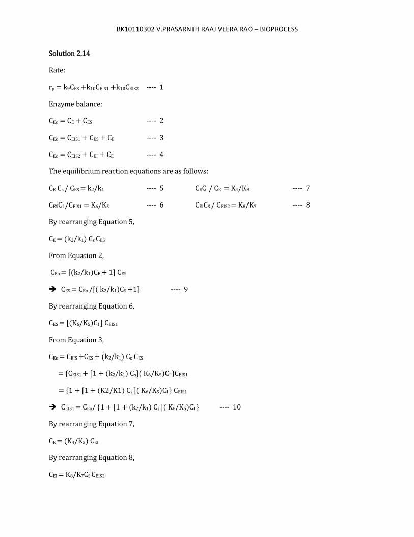
Solution 2.14
Rate:
rp = k9CES +k10CEIS1 +k10CEIS2 ---- 1
Enzyme balance:
CEo = CE + CES ---- 2
CEo = CEIS1 + CES + CE ---- 3
CEo = CEIS2 + CEI + CE ---- 4
The equilibrium reaction equations are as follows:
CE Cs / CES = k2/k1 ---- 5 CECI / CEI = K4/K3 ---- 7
CESCI /CEIS1 = K6/K5 ---- 6 CEICS / CEIS2 = K8/K7 ---- 8
By rearranging Equation 5,
CE = (k2/k1) Cs CES
From Equation 2,
CEo = [(k2/k1)CE + 1] CES
CES = CEo /[( k2/k1)CS +1] ---- 9
By rearranging Equation 6,
CES = [(K6/K5)CI ] CEIS1
From Equation 3,
CEo = CEIS +CES + (k2/k1) Cs CES
= {CEIS1 + [1 + (k2/k1) Cs]( K6/K5)CI }CEIS1
= {1 + [1 + (K2/K1) Cs ]( K6/K5)CI } CEIS1
CEIS1 = CEo/ {1 + [1 + (k2/k1) Cs ]( K6/K5)CI } ---- 10
By rearranging Equation 7,
CE = (K4/K3) CEI
By rearranging Equation 8,
CEI = K8/K7CS CEIS2
BK10110302 V.PRASARNTH RAAJ VEERA RAO – BIOPROCESS
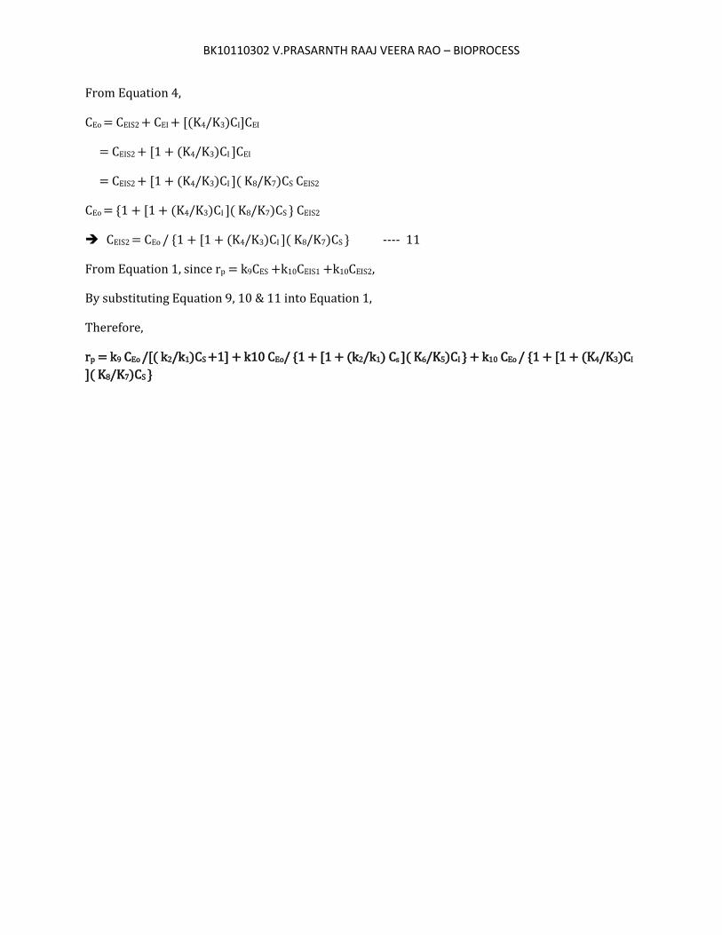
From Equation 4,
CEo = CEIS2 + CEI + [(K4/K3)CI]CEI
= CEIS2 + [1 + (K4/K3)CI ]CEI
= CEIS2 + [1 + (K4/K3)CI ]( K8/K7)CS CEIS2
CEo = {1 + [1 + (K4/K3)CI ]( K8/K7)CS } CEIS2
CEIS2 = CEo / {1 + [1 + (K4/K3)CI ]( K8/K7)CS } ---- 11
From Equation 1, since rp = k9CES +k10CEIS1 +k10CEIS2,
By substituting Equation 9, 10 & 11 into Equation 1,
Therefore,
rp = k9 CEo /[( k2/k1)CS +1] + k10 CEo/ {1 + [1 + (k2/k1) Cs ]( K6/K5)CI } + k10 CEo / {1 + [1 + (K4/K3)CI
]( K8/K7)CS }
BK10110302 V.PRASARNTH RAAJ VEERA RAO – BIOPROCESS
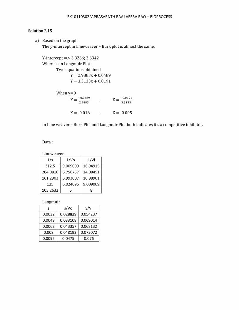
Solution 2.15
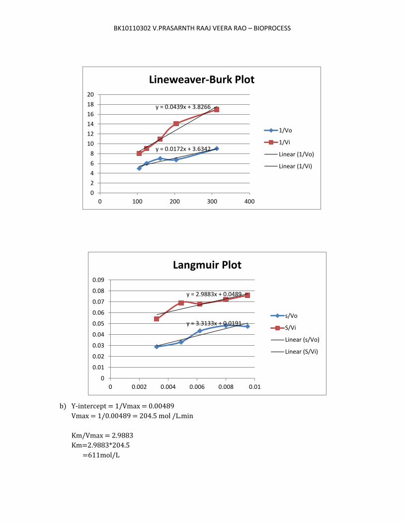
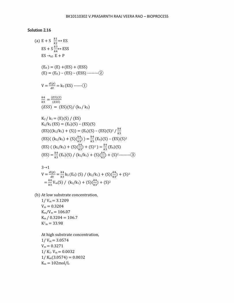
a) Based on the graphs
The y-intercept in Lineweaver – Burk plot is almost the same.
Y-intercept => 3.8266; 3.6342
Whereas in Langmuir Plot
Two equations obtained
Y = 2.9883x + 0.0489
Y = 3.3133x + 0.0191
When y=0
X =
; X =
X = -0.016 ; X = -0.005
In Line weaver – Burk Plot and Langmuir Plot both indicates it’s a competitive inhibitor
Data :
Lineweaver
1/s 1/Vo 1/Vi
312.5 9.009009 16.94915
204.0816 6.756757 14.08451
161.2903 6.993007 10.98901
125 6.024096 9.009009
105.2632 5 8
Langmuir
s s/Vo S/Vi
0.0032 0.028829 0.054237
0.0049 0.033108 0.069014
0.0062 0.043357 0.068132
0.008 0.048193 0.072072
0.0095 0.0475 0.076
BK10110302 V.PRASARNTH RAAJ VEERA RAO – BIOPROCESS
y = 0.0172x + 3.6342
y = 0.0439x + 3.8266
0
2
4
6
8
10
12
14
16
18
20
0 100 200 300 400
Lineweaver-Burk Plot
1/Vo
1/Vi
Linear (1/Vo)
Linear (1/Vi)
b) Y-intercept = 1/Vmax = 0.00489
Vmax = 1/0.00489 = 204.5 mol /L.min
Km/Vmax = 2.9883
Km=2.9883*204.5
=611mol/L
y = 3.3133x + 0.0191
y = 2.9883x + 0.0489
0
0.01
0.02
0.03
0.04
0.05
0.06
0.07
0.08
0.09
0 0.002 0.004 0.006 0.008 0.01
Langmuir Plot
s/Vo
S/Vi
Linear (s/Vo)
Linear (S/Vi)
BK10110302 V.PRASARNTH RAAJ VEERA RAO – BIOPROCESS
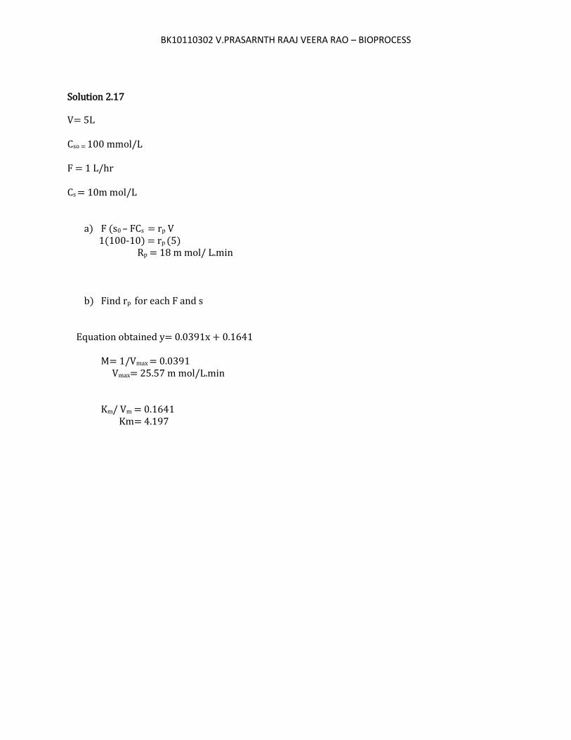
Solution 2.16
(a) E + S
↔
ES + S
↔
→k5 E + P
(E0 ) = (E) +(ES) + (ESS)
(E) = (E0 ) – (ES) – (ESS) --------
V = ( )
= k5 (ES) ------
= ( )( )
( )
( ) = (ES)(S)/ (k4 / k3)
K2 / k1 = (E)(S) / (ES)
K2/k1 (ES) = (E0)(S) – (ES)(S)
(ES)((k2/k1) + (S)) = (E0)(S) – (ES)(S)2 /
(ES)( (k2/k1) + (S)(
) ) =
(E0)(S) – (ES)(S)2
(ES) ( (k2/k1) + (S)(
) + (S)2 ) =
(E0)(S)
(ES) =
(E0)(S) / (k2/k1) + (S)(
) + (S)2 --------
3→
V = ( )
=
k5 (E0) (S) / (k2/k1) + (S)(
) + (S)2
=
Vm(S) / (k2/k1) + (S)(
) + (S)2
(b) At low substrate concentration,
1/ Vm = 3.1209
Vm = 0.3204
Km/Vm = 106.07
Km / 0.3204 = 106.7
K1m = 33.98
At high substrate concentration,
1/ Vm = 3.0574
Vm = 0.3271
1/ K1. Vm = 0.0032
1/ Km(3.0574) = 0.0032
Km = 102mol/L
BK10110302 V.PRASARNTH RAAJ VEERA RAO – BIOPROCESS
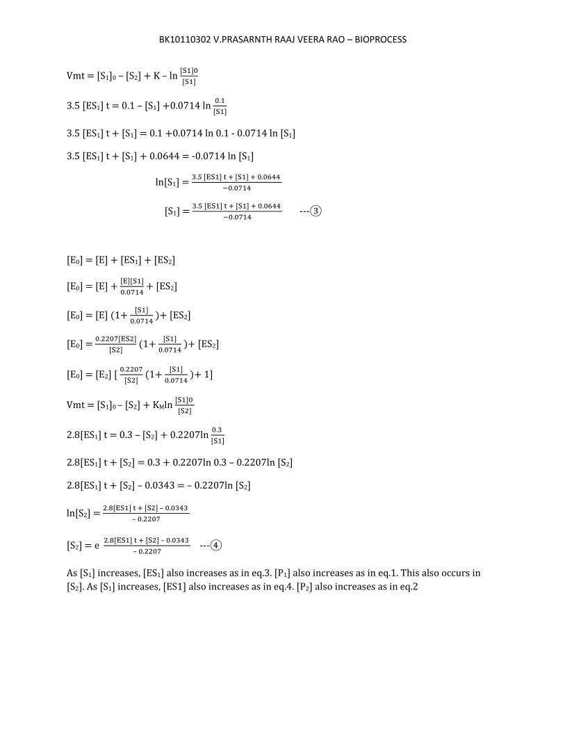
Solution 2.17
V= 5L Cso = 100 mmol/L F = 1 L/hr Cs = 10m mol/L
a) F (s0 – FCs = rp V 1(100-10) = rp (5) Rp = 18 m mol/ L.min
b) Find rp for each F and s Equation obtained y= 0.0391x + 0.1641 M= 1/Vmax = 0.0391 Vmax= 25.57 m mol/L.min Km/ Vm = 0.1641 Km= 4.197

BK10110302 V.PRASARNTH RAAJ VEERA RAO – BIOPROCESS
Solution 2.18
[SO]1 = 0.1 mol/L [S0]2 = 0.3mol/L [E0] = 0.05 mol/L
[ ][ ]
[ ]
[ ][ ]
[ ]
[ ][ ]
[ ]
[ ][ ]
[ ]
[ ][ ]
[ ]
[ ][ ]
[ ]
V1 = [ ]
= k5[ES1]
=3.5 [ES1] ---
V2 = [ ]
= k6[ES2]
=2.8 [ES2] ---
[E0] = [E] + [ES1] + [ES2]
[E0] = [E] + [ES1] + [ ][ ]
[E0] = [ES1] + [E] (1+[ ]
)
[E0] = [ES1] + [ ]
[ ] (1+
[ ]
)
[E0] = [ES1] {1 +
[ ] (1+
[ ]
)}
[ES1] = [ ]
[ ] (
[ ]
)
BK10110302 V.PRASARNTH RAAJ VEERA RAO – BIOPROCESS
Vmt = [S1]0 – [S2] + K – ln [ ]
[ ]
3.5 [ES1] t = 0.1 – [S1] +0.0714 ln
[ ]
3.5 [ES1] t + [S1] = 0.1 +0.0714 ln 0.1 - 0.0714 ln [S1]
3.5 [ES1] t + [S1] + 0.0644 = -0.0714 ln [S1]
ln[S1] = [ ] [ ]
[S1] = [ ] [ ]
---
[E0] = [E] + [ES1] + [ES2]
[E0] = [E] + [ ][ ]
+ [ES2]
[E0] = [E] (1+ [ ]
)+ [ES2]
[E0] = [ ]
[ ] (1+
[ ]
)+ [ES2]
[E0] = [E2] [
[ ] (1+
[ ]
)+ 1]
Vmt = [S1]0 – [S2] + KMln [ ]
[ ]
2.8[ES1] t = 0.3 – [S2] + 0.2207ln
[ ]
2.8[ES1] t + [S2] = 0.3 + 0.2207ln 0.3 – 0.2207ln [S2]
2.8[ES1] t + [S2] – 0.0343 = – 0.2207ln [S2]
ln[S2] = [ ] [ ] –
–
[S2] = e [ ] [ ] –
– ---
As [S1] increases, [ES1] also increases as in eq.3. [P1] also increases as in eq.1. This also occurs in
[S2]. As [S1] increases, [ES1] also increases as in eq.4. [P2] also increases as in eq.2
BK10110302 V.PRASARNTH RAAJ VEERA RAO – BIOPROCESS
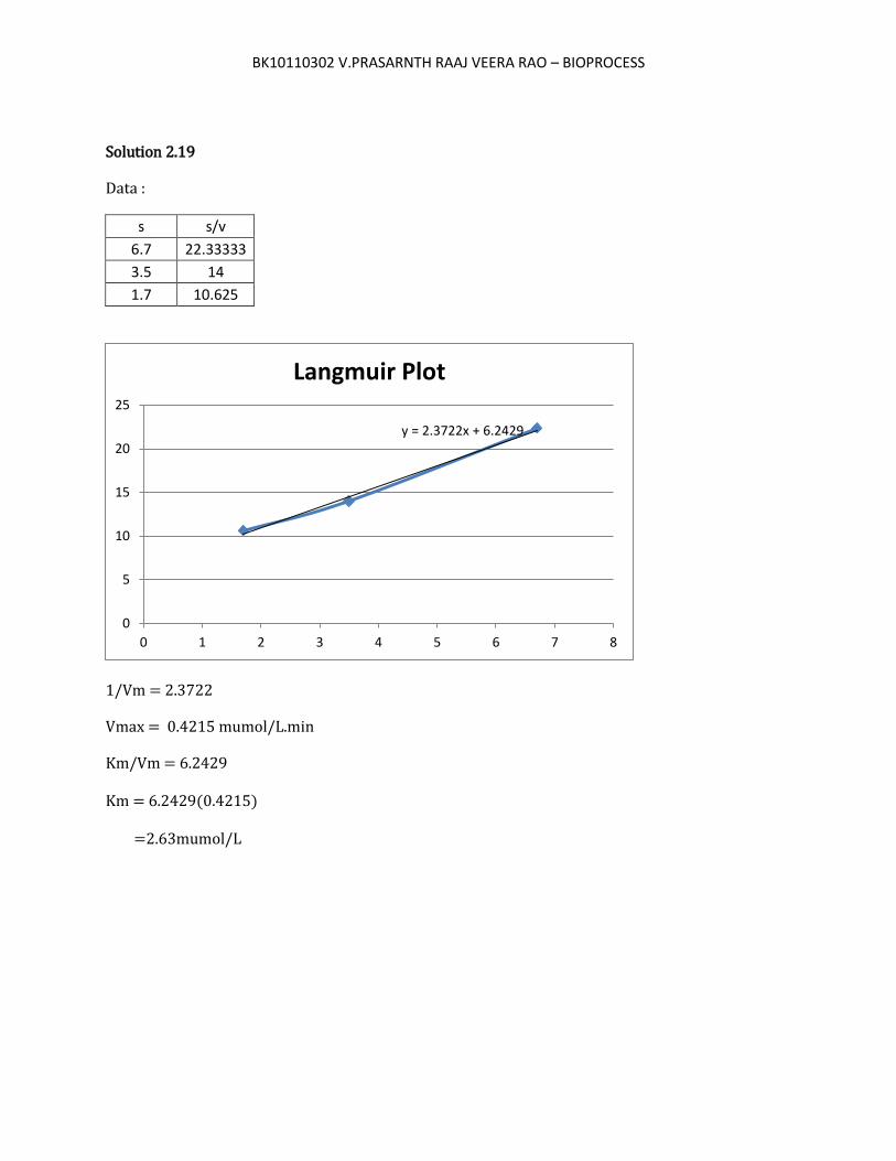
Solution 2.19
Data :
s s/v
6.7 22.33333
3.5 14
1.7 10.625
1/Vm = 2.3722
Vmax = 0.4215 mumol/L.min
Km/Vm = 6.2429 Km = 6.2429(0.4215) =2.63mumol/L
y = 2.3722x + 6.2429
0
5
10
15
20
25
0 1 2 3 4 5 6 7 8
Langmuir Plot
BK10110302 V.PRASARNTH RAAJ VEERA RAO – BIOPROCESS
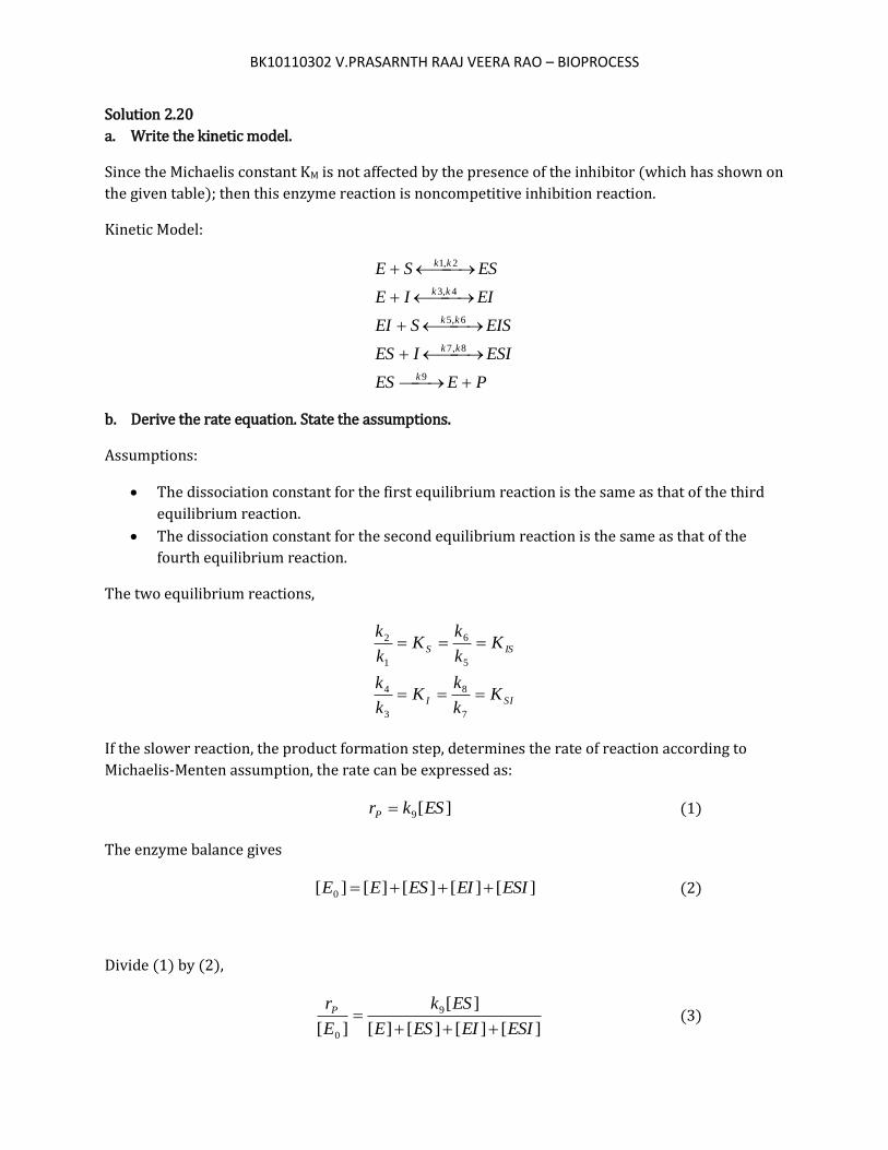
Solution 2.20
a. Write the kinetic model.
Since the Michaelis constant KM is not affected by the presence of the inhibitor (which has shown on
the given table); then this enzyme reaction is noncompetitive inhibition reaction.
Kinetic Model:
PEES
ESIIES
EISSEI
EIIE
ESSE
k
kk
kk
kk
kk
9
8,7
6,5
4,3
2,1
b. Derive the rate equation. State the assumptions.
Assumptions:
The dissociation constant for the first equilibrium reaction is the same as that of the third
equilibrium reaction.
The dissociation constant for the second equilibrium reaction is the same as that of the
fourth equilibrium reaction.
The two equilibrium reactions,
SII
ISS
Kk
kK
k
k
Kk
kK
k
k
7
8
3
4
5
6
1
2
If the slower reaction, the product formation step, determines the rate of reaction according to
Michaelis-Menten assumption, the rate can be expressed as:
][9 ESkrP (1)
The enzyme balance gives
][][][][][ 0 ESIEIESEE (2)
Divide (1) by (2),
][][][][
][
][
9
0 ESIEIESE
ESk
E
rP
(3)
BK10110302 V.PRASARNTH RAAJ VEERA RAO – BIOPROCESS
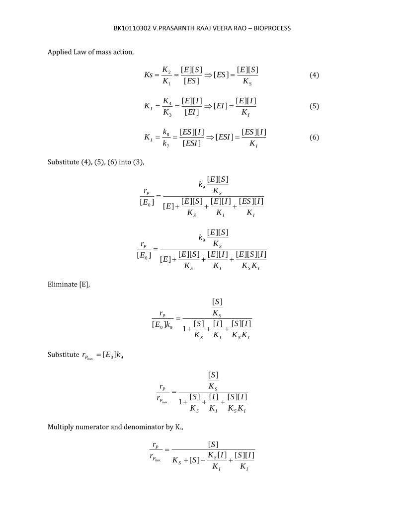
Applied Law of mass action,
SK
SEES
ES
SE
K
KKs
]][[][
][
]][[
1
2 (4)
I
IK
IEEI
EI
IE
K
KK
]][[][
][
]][[
3
4 (5)
I
IK
IESESI
ESI
IES
k
kK
]][[][
][
]][[
7
8 (6)
Substitute (4), (5), (6) into (3),
IIS
SP
K
IES
K
IE
K
SEE
K
SEk
E
r
]][[]][[]][[][
]][[
][
9
0
ISIS
SP
KK
ISE
K
IE
K
SEE
K
SEk
E
r
]][][[]][[]][[][
]][[
][
9
0
Eliminate [E],
ISIS
SP
KK
IS
K
I
K
S
K
S
kE
r
]][[][][1
][
][ 90
Substitute 90 ][max
kErP
ISIS
S
P
P
KK
IS
K
I
K
S
K
S
r
r
]][[][][1
][
max
Multiply numerator and denominator by Ks,
II
SS
P
P
K
IS
K
IKSK
S
r
r
]][[][][
][
max
BK10110302 V.PRASARNTH RAAJ VEERA RAO – BIOPROCESS
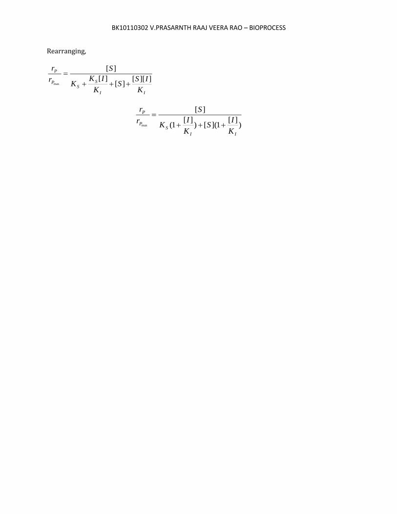
Rearranging,
II
SS
P
P
K
ISS
K
IKK
S
r
r
]][[][
][
][
max
)][
1]([)][
1(
][
max
II
SP
P
K
IS
K
IK
S
r
r