Isotropic Markov semigroups on ultra-metric spaces∗

Alexander Bendikov† Alexander Grigor’yan‡ Christophe Pittet§

Wolfgang Woess¶

Dedicated to the memories ofV.S. Vladimirov (1923–2012) and M.H. Taibleson (1929–2004)

Abstract

Let (X, d) be a separable ultra-metric space with compact balls. Given a reference mea-sure μ on X and a distance distribution function σ on [0 , ∞), we construct a symmetricMarkov semigroup {P t}t≥0 acting in L2(X,μ). Let {Xt} be the corresponding Markov pro-cess. We obtain upper and lower bounds of its transition density and its Green function,give a transience criterion, estimate its moments and describe the Markov generator L andits spectrum which is pure point. In the particular case when X = Qn

p , where Qp is the fieldof p-adic numbers, our construction recovers the Taibleson Laplacian (spectral multiplier),and we can also apply our theory to the study of the Vladimirov Laplacian. Even in this wellestablished setting, several of our results are new. We also elaborate the relation betweenthe Markov process {Xt} and Kigami’s process on the boundary of a tree, which is inducedby a random walk on the tree. In conclusion, we provide examples illustrating the interplaybetween the fractional derivatives and random walks.

Contents

1 Introduction 2

2 Isotropic semigroup and the heat kernel 72.1 Averaging operator . . . . . . . . . . . . . . . . . . . . . . . . . . . . . . . . . . . 72.2 Basic properties of isotropic semigroup . . . . . . . . . . . . . . . . . . . . . . . . 82.3 Spectral distribution function . . . . . . . . . . . . . . . . . . . . . . . . . . . . . 112.4 Estimates of the heat kernel . . . . . . . . . . . . . . . . . . . . . . . . . . . . . . 152.5 Heat kernels in Qp . . . . . . . . . . . . . . . . . . . . . . . . . . . . . . . . . . . 192.6 Green function and transience . . . . . . . . . . . . . . . . . . . . . . . . . . . . . 21

3 Isotropic Laplacian and its spectrum 243.1 Subordination . . . . . . . . . . . . . . . . . . . . . . . . . . . . . . . . . . . . . . 243.2 L2-spectrum . . . . . . . . . . . . . . . . . . . . . . . . . . . . . . . . . . . . . . . 253.3 The Dirichlet form and jump kernel . . . . . . . . . . . . . . . . . . . . . . . . . 293.4 Lp-spectrum . . . . . . . . . . . . . . . . . . . . . . . . . . . . . . . . . . . . . . . 31

4 Moments of the isotropic Markov process 33

∗Version of June 16, 2014. Mathematics Subject Classification: 05C05, 47S10, 60J25, 81Q10†Supported by the Polish Government Scientific Research Fund, Grant 2012/05/B/ST 1/00613‡Supported by SFB 701 of German Research Council§Supported by the CNRS, France¶Supported by Austrian Science Fund projects FWF W1230-N13 and FWF P24028-N18

1

5 Analysis in Qp and Qnp 39

5.1 The p-adic fractional derivative . . . . . . . . . . . . . . . . . . . . . . . . . . . . 395.2 Rotation invariant Markov semigroups . . . . . . . . . . . . . . . . . . . . . . . . 425.3 Product spaces . . . . . . . . . . . . . . . . . . . . . . . . . . . . . . . . . . . . . 45

5.3.1 The Vladimirov Laplacian . . . . . . . . . . . . . . . . . . . . . . . . . . . 475.3.2 The Taibleson Laplacian . . . . . . . . . . . . . . . . . . . . . . . . . . . . 51

6 Random walks on a tree and jump processes on its boundary 536.1 Rooted trees and their boundaries . . . . . . . . . . . . . . . . . . . . . . . . . . 536.2 Isotropic jump processes on the boundary of a tree . . . . . . . . . . . . . . . . . 556.3 Nearest neighbour random walks on a tree . . . . . . . . . . . . . . . . . . . . . . 566.4 Harmonic functions of finite energy and their boundary values . . . . . . . . . . . 576.5 Jump processes on the boundary of a tree . . . . . . . . . . . . . . . . . . . . . . 58

7 The duality of random walks on trees and isotropic processeson their boundaries 627.1 Answer to Question I . . . . . . . . . . . . . . . . . . . . . . . . . . . . . . . . . . 637.2 Answer to Question II . . . . . . . . . . . . . . . . . . . . . . . . . . . . . . . . . 657.3 The non-compact case . . . . . . . . . . . . . . . . . . . . . . . . . . . . . . . . . 68

8 Random walk associated with p-adic fractional derivative 738.1 The p-adic fractional derivative on Zp . . . . . . . . . . . . . . . . . . . . . . . . 738.2 Nearest neighbour random walk on the rooted tree To

p . . . . . . . . . . . . . . . 758.3 The random walk corresponding to Dα on Qp . . . . . . . . . . . . . . . . . . . . 77

1 Introduction

In the past three decades there has been an increasing interest in various constructions of Markovchains on ultra-metric (totally disconnected) spaces, such as the Cantor set or the field of p-adicnumbers. In this paper we introduce and study a class of symmetric Markov semigroups andtheir generators on ultra-metric spaces. Our construction is very transparent, and it leads to anumber of new results as well as to a better understanding of previously known results.

Let (X, d) be a metric space. The metric d is called an ultra-metric if it satisfies the ultra-metric inequality

d(x, y) ≤ max{d(x, z), d(z, y)}, (1.1)

that is obviously stronger than the usual triangle inequality. In this case (X, d) is called anultra-metric space.

We will always assume in addition that the ultra-metric space (X, d) in question is separable,and that every closed ball

Br(x) = {y ∈ X : d(x, y) ≤ r} (1.2)

is compact. The latter implies that (X, d) is complete.The ultra-metric property (1.1) implies that the balls in an ultra-metric space (X, d) look

very differently from familiar Euclidean balls. In particular, any two ultra-metric balls of thesame radius are either disjoint or identical. Consequently, the collection of all distinct balls ofthe same radius r forms a partition of X.

One of the best known examples of an ultra-metric space is the field Qp of p-adic numbersendowed with the p-adic norm ‖x‖p and the p-adic ultra-metric d(x, y) = ‖x − y‖p . Moreover,

2

for any integer n ≥ 1, the p-adic n-space Qnp = Qp × ... ×Qp is also an ultra-metric space with

the ultra-metric dn(x, y) defined as

dn(x, y) = max{d(x1, y1), ..., d(xn, yn)}.

If the group of isometries of an ultra-metric space (X, d) acts transitively on X, then (X, d)is in fact a locally compact Abelian group, which in particular is the case for Qn

p .In literature one distinguishes the following two subclasses of ultra-metric spaces:

(i) (X, d) is discrete and infinite.

(ii) (X, d) is perfect (that is, X contains no isolated point).

Various constructions of Markov processes in the setting (ii), when X in addition is a locallycompact Abelian group, have been developed by Evans [22], Haran [29], [30], Ismagilov [33],Kochubei [38], [39], Albeverio and Karwowski [1], [2], Albeverio and Zhao [3], Del Muto andFiga-Talamanca [42], [43], Rodrigues-Vega and Zuniga-Galindo [66], [50]. They studied X-valuedinfinitely divisible random variables and processes by using tools of Fourier analysis; for generalreferences, see Hewitt and Ross [31], Taibleson [55] and Kochubei [39]. Note that Taibleson’sspectral multipliers on Qn

p are early forerunners of the Laplacians that we are considering here.Pearson and Bellissard [45] and Kigami [36], [37] considered random walks on the Cantor

set, resp. the Cantor set minus one point. In [36], [37], a main focus is on the interplay betweenrandom walks on trees and jump process on their boundaries. In this context, we also mentionAldous and Evans [4] and Chen, Fukushima and Ying [15]. We shall come back to Kigami’swork in the last three sections of this paper.

An entirely different approach was developed by Vladimirov, Volovich and Zelenov [57], [59].They were concerned with p-adic analysis (Bruhat distributions, Fourier transform etc.) relatedto the concept of p-adic Quantum Mechanics, and introduced a class of pseudo-differentialoperators on Qp and on Qn

p . In particular, they studied the p-adic Laplacian defined on Q3p

and the corresponding p-adic Schrodinger equation. In particular, they explicitly computed (asseries expansions) certain heat kernels as well as the Green function of the p-adic Laplacian.In connection with the theory of pseudo-differential operators on general totally disconnectedgroups we mention here the pioneering work of Saloff-Coste [51].

Discrete ultra-metric spaces (X, d) (as in (i)) were treated by Bendikov, Grigor’yan andPittet [7], the direct forerunner of the present work. Among the examples of such spaces wemention the class of locally finite groups: a countable group G is locally finite if any of its finitesubsets generates a finite subgroup. Every locally finite group G is the union of an increasingsequence of finite subgroups {Gn}. An ultra-metric d in G can be defined as follows: d(x, y) isthe minimal value of n such that x and y belong to a common coset of Gn .

Since locally finite groups are not finitely generated, the basic notions of geometric grouptheory such as the word metric, volume growth, isoperimetric inequalities, etc. (cf. e.g. [16],[28], [52], [46], [47], [48], , [56], [61]), do not apply in this setting. The notion of an ultra-metriccan be used instead of the word metric in this setting (see [5], [7], [6]).

Selecting a set of generators for each subgroup Gn of a locally finite group G, one de-fines thereby a random walk, that is, a Markov kernel on Gn. Taking a convex combina-tion of the Markov kernels across all Gn, one obtains a Markov kernel on G that determinesa random walk on G . Such random walks have been studied by Darling and Erdos [17],Kesten and Spitzer [35], Flatto and Pitt [26], Fereig and Molchanov [25], Kasymdzhanova [34],Cartwright [13], Lawler [40], Brofferio and Woess [11], see also Bendikov and Saloff-Coste [9]. Inparticular, [40] has a remarkable general criterion of recurrence of such random walks. Furtherresults on Markov processes on ultra-metric spaces can be found in [18], [19], [23], [24], [41], [49].

3

Many of the results in the above-mentioned literature are covered by our approach via ultra-metrics. We develop tools to analyse a natural class of Markov processes on ultra-metric spaceswithout assuming any group structure. In particular, the nature of our argument allows us tobring into consideration an arbitrary Radon measure μ on X (instead of the Haar measure inthe case of groups), that is used as a speed measure for a Markov process.

So, given an ultra-metric space (X, d), fix a Radon measure μ on X with full support anddefine the family {Qr}r>0 of averaging operators acting on non-negative or bounded Borel func-tions f : X → R by

Qrf(x) =1

μ (Br(x))

∫

Br(x)f dμ. (1.3)

Note that 0 < μ (Br (x)) < ∞ for all x ∈ X and r > 0. The operator Qr has the kernel

Kr(x, y) =1

μ (Br(x))1Br(x)(y). (1.4)

It is symmetric in x, y because Br(x) = Br(y) for any y ∈ Br(x). Clearly, Qr is a Markovoperator on the space Bb (X) of bounded Borel functions on X, that is, Qrf ≥ 0 if f ≥ 0 andQr1 = 1. Hence, Qr extends to a bounded self-adjoint operator in L2 (X,μ) .

Let us choose a function σ that satisfies the following assumptions:

σ : [0,∞] → [0, 1] is a strictly monotone increasingleft-continuous function, such that σ (0+) = 0 and σ (∞) = 1.

(1.5)

Then the operator

Pf =∫ ∞

0Qrf dσ(r) (1.6)

is also a Markov operator in Bb (X) as well as a bounded self-adjoint operator in L2 (X,μ).The operator P determines a discrete time Markov chain {Xn}n∈N on X with the following

transition rule: a random point Xn+1 is μ-uniformly distributed in Br(Xn) where the radius ris chosen at random according to the probability distribution σ. For that reason we refer to σas the distance distribution function.

Note that the operator P is determined by the triple (d, μ, σ) . We refer to P as an isotropicMarkov operator associated with (d, μ, σ). The isotropic Markov operator P has some uniquefeatures arising from the ultra-metric property. First of all, let us mention the following simpleidentity:

Qr Qs = Qs Qr = Qmax{r,s}. (1.7)

Indeed, for any ball B of radius r, any point x ∈ B is a center of B. Since the value Qrf (x)is the average of f in B, we see that Qrf (x) does not depend on x ∈ B; that is, Qrf = conston B. Now, if s ≤ r then the application of Qs to Qrf does not change this constant, whencewe obtain QsQrf = Qrf. On the other hand, if s > r then any ball of radius s is the disjointunion of finitely many balls of radius r. Since the integrals of f and Qrf over any such ball arethe same, we obtain QsQrf = Qsf.

Since by (1.7) Q2r = Qr, we obtain that Qr is an orthoprojector 1 in L2. In particular,

specQr ⊂ [0, 1] .It follows from (1.6) that the spectral projectors in the spectral decomposition of P are

the averaging operators Qr, up to a change of variables (cf. (2.6). The fact that the spectralprojectors are themselves Markov operators brings up a new insight, new technical possibilities,and a new type of results, that have no analogue in other commonly used settings.

1Let us mention for comparison, that the analogous averaging operator in Rn is also bounded and self-adjoint,but it has a non-empty negative part of the spectrum. In particular, it is not an orthoprojector.

4

In particular, the Markov operator P is non-negative definite, which allows us to define thepowers P t for all t ≥ 0. Then

{P t}

t≥0is a symmetric strongly continuous Markov semigroup.

It follows from (1.6) that P t admits for t > 0 the following representation:

P tf(x) =∫ ∞

0Qrf(x) dσt(r) . (1.8)

Alternatively, one can define P t by (1.8) and then use formula (1.7) to derive that P sP t = P s+t.The semigroup

{P t}

t≥0determines a continuous time Markov process {Xt}t≥0 . Since the

n-step transition operator of the discrete time Markov chain {Xn}n∈N is Pn, we see that thediscrete time Markov chain coincides with the restriction of the continuous time Markov process{Xt} to integer values of t. This allows us to concentrate on the study of the continuous timeprocess {Xt}t≥0 only.

We refer to the Markov semigroup{P t}

t≥0defined by (1.3)-(1.8) as an isotropic semigroup,

and to the jump process {Xt}t≥0 as an isotropic process, associated with the triple (d, μ, σ).Let us briefly describe the content of the present paper that is devoted to the study of

isotropic semigroups.In Section 2 we construct the isotropic semigroup as above and provide explicit formulas

for its heat kernel p (t, x, y) (=the transition density of the process {Xt}). As indicated above,our approach is based upon the observation that the building blocks of the operator P , namely,the averaging operators Qr of (1.3), are orthogonal projectors in L2(X,μ), which enables us toengage at an early stage the methods of spectral theory and functional calculus.

We establish some basic properties of the heat kernel, for example, its continuity away fromthe diagonal, and prove upper and lower bounds in terms of t and d (x, y).

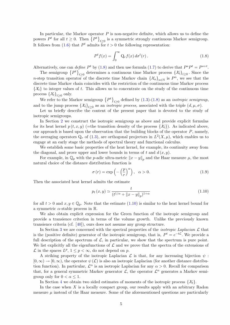
For example, in Qp with the p-adic ultra-metric ‖x − y‖p and the Haar measure μ, the mostnatural choice of the distance distribution function is

σ (r) = exp(−(p

r

)α), α > 0. (1.9)

Then the associated heat kernel admits the estimate

pt (x, y) 't

(t1/α + ‖x − y‖p)1+α

(1.10)

for all t > 0 and x, y ∈ Qp. Note that the estimate (1.10) is similar to the heat kernel bound fora symmetric α-stable process in R.

We also obtain explicit expression for the Green function of the isotropic semigroup andprovide a transience criterion in terms of the volume growth. Unlike the previously knowntransience criteria (cf. [40]), ours does not assume any group structure.

In Section 3 we are concerned with the spectral properties of the isotropic Laplacian L thatis the (positive definite) generator of the isotropic semigroup, that is, P t = e−tL. We provide afull description of the spectrum of L, in particular, we show that the spectrum is pure point.We list explicitly all the eigenfunctions of L and we prove that the spectra of the extensions ofL in the spaces Lp, 1 ≤ p < ∞, do not depend on p.

A striking property of the isotropic Laplacian L is that, for any increasing bijection ψ :[0,∞) → [0,∞), the operator ψ (L) is also an isotropic Laplacian (for another distance distribu-tion function). In particular, Lα is an isotropic Laplacian for any α > 0. Recall for comparisonthat, for a general symmetric Markov generator L, the operator Lα generates a Markov semi-group only for 0 < α ≤ 1.

In Section 4 we obtain two sided estimates of moments of the isotropic process {Xt}.In the case when X is a locally compact group, our results apply with an arbitrary Radon

measure μ instead of the Haar measure. Some of the aforementioned questions are particularly

5

sensitive to the choice of the measure μ, for example, the heat kernel and Green functionestimates. On the other hand, the spectrum of the Laplacian and the moment bounds do notdepend on μ. These quantities depend strongly on the choice of the ultra-metric d, whereas theeigenfunctions depend both on d and μ.

In Section 5 we compare our isotropic Laplacian with other previously known “differential”operators in Qp and Qn

p . The notion of fractional derivative Dα on functions on Qp was intro-duced by Vladimirov [57] by means of Fourier transform in Qp. The operator Dα coincides withthe operator of Taibleson [55], introduced in a quite different context of Riesz multipliers onQn

p . We show that Dα coincides with our isotropic Laplacian Lα associated with the distancedistribution function (1.9). In particular, this implies that the heat kernel of Dα satisfies theestimate (1.10). Note that previously only an upper bound for the heat kernel of Dα was known(cf. Kochubei [39, Ch.4.1, Lemma 4.1]). We also give a simple proof for a previously knownexplicit formula for the Green function of Dα.

Using functional calculus of the operator D1, we give a full description of the class of allrotation invariant Markov generators on Qp. This class includes but is not restricted to theisotropic Laplacians. As a consequence, we obtain that the class of all rotation invariant Markovprocesses in Qp coincides with the class of Markov processes constructed by Albeverio andKarwowski [2] by use of much more involved technical tools.

Next we consider “partial differential” operators on Qnp . The p-adic Laplacian of Vladimirov

on Qnp is defined as a direct sum of the operators Dα acting separately on each coordinate.

Although this operator is not an isotropic Laplacian, it can be studied within our setting, whichgives simple direct proofs of many results of [59], without using Fourier Analysis and the theoryof Bruhat distributions.

Another multidimensional generalization of Dα is the Taibleson operator Tα in Qnp that is

defined by means of Fourier transform in Qnp . We show that the operator Tα is an isotropic

Laplacian, which allows to obtain detailed analytic results.In Section 6 we use the fact that every locally compact ultra-metric space arises as the

boundary of a locally finite tree. Using that we relate random walks2 on the tree with isotropicjump processes on its boundary. Kigami in [36] starts with a transient nearest neighbour randomwalk on a tree and constructs a naturally associated jump process on the boundary of the tree:given the Dirichlet form of the random walk on the tree, the boundary process is induced by theDirichlet form that reproduces the energy of a harmonic function on the tree via its boundaryvalues. This is analogous to the well-known Douglas integral [21] on the unit disk. Using thisapproach, [36] undertakes a detailed analysis of the process on the boundary.

Restricting attention at first to the compact case, we answer in Section 7 the obvious questionhow the approach of Kigami and that of the present paper are related. The relation is basicallyone-to-one: every boundary process induced by a random walk is an isotropic process in oursense. Conversely, we show that, up to a unique linear time change, every isotropic process onthe boundary of a tree arises from a uniquely determined random walk on the tree as in [36]. Inaddition, we explain how the boundary process on a tree transforms into an isotropic processon the non-compact ultra-metric space given by a punctured boundary of the tree. This shouldbe compared with [37].

Finally, in Section 8 we construct explicitly the random walks on the trees, which correspondto fractional derivatives on the (compact) group Zp of p-adic integers and on the whole of Qp.

Acknowledgement. This work was begun and finished at Bielefeld University under sup-port of SFB 701 of the German Research Council. The authors thank S. Albeverio, J. Bellissard,P. Diaconis, W. Herfort, A.N. Kochubei, S.A. Molchanov, L. Saloff-Coste, I.V. Volovich andE.I. Zelenov for fruitful discussions and valuable comments.

2Discrete time random walks of nearest neighbour type on a tree are very well understood – see the book byWoess [63, Ch. 9]

6

2 Isotropic semigroup and the heat kernel

Throughout this paper, (X, d) is an ultra-metric space which is separable, and such that alld-balls Br (x) are compact.

2.1 Averaging operator

Recall that for any r > 0,

Qrf(x) =1

μ (Br(x))

∫

Br(x)f dμ

is an orthoprojector in L2 ≡ L2 (X,μ) (cf. (1.3)), and the image of Qr is the subspace Vr of L2

that consists of all functions taking constant values on each ball radius r.Clearly, the family {Vr}r>0 is monotone decreasing with respect to set inclusion. It follows

that there exists the limitQ∞ := s- lim

r→∞Qr

in the strong operator topology, which is an orthoprojector onto V∞ =⋂

r>0 Vr. It follows thatV∞ consists of constant functions. If μ (X) = ∞ then V∞ = {0} and Q∞ = 0, while in the caseμ (X) < ∞ we have dimV∞ = 1 and

Q∞f =1

μ (X)

∫

Xfdμ. (2.1)

Set also Q0 := id .

Lemma 2.1 The family {Qr}r∈[0,∞) of orthoprojectors is strongly right continuous in r.

Proof. Let us first show that r 7→ Qr is strongly continuous at r = 0, that is,

s- lims→0+

Qs = id . (2.2)

Let f be a continuous function on X with compact support. Then, for any x ∈ X,

Qsf (x) → f (x) as s → 0.

Since the family {Qsf}s∈(0,1) is uniformly bounded by sup |f | and is uniformly compactly sup-ported, it follows by the dominated convergence theorem that

‖Qsf − f‖L2 → 0 as s → 0. (2.3)

Since the space of continuous functions with compact support is dense in L2, by a standardapproximation argument (2.3) extends to all f ∈ L2, whence (2.2) follows.

Next, let us prove that r 7→ Qr is strongly right continuous at any r > 0, that is,

s- lims→r+

Qs = Qr. (2.4)

It suffices to show that, for any continuous function f with compact support,

‖Qsf − Qrf‖L2 → 0 as s → r+ . (2.5)

Indeed, for any x ∈ X, the function r 7→ Qrf (x) is right continuous by (1.3) as the balls areclosed, whence (2.5) follows by the dominated convergence theorem.

7

For any λ ∈ R set

Eλ =

{Q1/λ, λ > 0,

0, λ ≤ 0.(2.6)

Note that E0+ = Q∞. It follows from the above properties of Qr that the family {Eλ} of ortho-projectors in L2 is a left-continuous spectral resolution. Consequently, for any Borel functionϕ : [0,∞) → R, the integral ∫

[0,∞)ϕ (λ) dEλ

determines a self-adjoint non-negative definite operator, which is bounded if and only if ϕ isbounded.

2.2 Basic properties of isotropic semigroup

Consider now the operator P defined by (1.6) with a function σ as in (1.5). Observe that theintegral in (1.6) converges in the strong operator topology since, for any f ∈ L2,

∫ ∞

0‖Qrf‖L2 dσ (r) < ∞.

On the other hand, for any f ∈ Bb (X), the integral (1.6) converges pointwise. Moreover, in thiscase the function Pf is continuous, because the function x 7→

∫∞ε Qrf (x) dσ (r) is for any ε > 0

locally constant and, hence, continuous and it converges uniformly to Pf (x) as ε → 0.As it was already observed, P is a self-adjoint operator in L2 and spec P ⊂ [0, 1] . In

particular, for any t > 0, the power P t is well defined. Set also P 0 := id. In the next statementwe collect basic properties of P t.

Theorem 2.2 (a) The family {P t}t≥0 is a strongly continuous symmetric Markov semigroupon L2(X,μ).

(b) For any t > 0, the operator P t has the representation (1.8), that is,

P tf =∫

[0,∞)Qrf dσt(r) .

(c) For any t > 0, the operator P t admits an integral kernel p(t, x, y), that is, for all f ∈ Bb

and f ∈ L2,

P tf(x) =∫

Xp(t, x, y)f(y)dμ(y), (2.7)

where p (t, x, y) is given by

p(t, x, y) =∫

[d(x,y),∞)

dσt(r)μ (Br(x))

. (2.8)

The function p (t, x, y) is called the heat kernel of the semigroup{P t}. It is clear from (2.8)

that p (t, x, y) < ∞ for all t > 0 and x 6= y, whereas under certain conditions p (t, x, x) can beequal to ∞.

For f ∈ Bb the identity (2.7) holds pointwise, that is, for all x ∈ X, whereas for f ∈ L2 (2.7)is an identity of two L2-functions, that it, it holds for μ-almost all x.Proof. It follows from (1.6) by integration by parts that, for any f ∈ L2,

Pf =∫

[0,∞)Qrf dσ(r) = Q∞f −

∫

(0,∞)σ (r) dQrf. (2.9)

8

Changing λ = 1/r and using (2.6), we obtain

Pf = (E0+) f +∫

(0,∞)σ (1/λ) dEλf =

∫

[0,∞)σ (1/λ) dEλf,

using the convention σ (∞) = 1. Hence, we obtain the spectral decomposition of P in thefollowing form:

P =∫

[0,∞)σ (1/λ) dEλ. (2.10)

It follows that

P t =∫

[0,∞)σt (1/λ) dEλ. (2.11)

(a) The semigroup identity P tP s = P t+s is a straightforward consequence of (2.11) and thefunctional calculus. The strong continuity condition

s- limt→0+

P t = id

follows also from (2.11) because σ (1/λ) > 0 for λ ∈ [0,∞) and, hence, σt (1/λ) → 1 as t → 0+.(b) Reversing the argument in the derivation of (2.11) from (2.9), we obtain that (2.11)

implies

P tf =∫

[0,∞)Qrf dσt(r).

(c) It follows from (b), (1.3) and Fubini that, for any f ∈ Bb,

P tf (x) =∫

[0,∞)

(1

μ (Br(x))

∫

X1Br(x) (y) f(y)dμ(y)

)

dσt(r)

=∫

X

(∫

[d(x,y),∞)

1μ (Br(x))

dσt(r)

)

f(y)dμ(y)

=∫

Xp (t, x, y) f (y) dμ (y) .

For f ∈ L2 it follows by approximation argument.

Remark 2.3 In the proof of Theorem 2.2 we have not used at full strength the fact that σis strictly monotone increasing (cf. (1.5)). For that theorem, it suffices to assume that σ ismonotone increasing and σ (r) > 0 for r > 0.

Remark 2.4 If one takes (1.8) as definition of the operator P t, then one can prove the semi-group identity P tP s = P t+s by means of (1.7). Indeed, for any given s, t > 0 and f ∈ L2, wehave

P sP tf(x) =∫ ∞

0dσs(r)

∫ ∞

0dσt(r′)QrQr′f(x) =

=∫ ∞

0dσs(r)

∫ ∞

0dσt(r′)Qmax{r,r′}f(x).

Let ξ1 and ξ2 be two independent random variables with distributions σs and σt, respectively.Then the distribution of the random variable ξ = max{ξ1, ξ2} is σt+s. It follows that

P sP tf(x) = E(Qmax{ξ1,ξ2}f(x)

)=∫ ∞

0Qrf(x) dσt+s(r) = P t+sf(x).

9

Corollary 2.5 For all x, y ∈ X and t > 0, we have p (t, x, y) > 0,

p (t, x, y) = p (t, y, x) ,

andp(t, x, y) ≤ min{p(t, x, x), p(t, y, y)}. (2.12)

Proof. The strict positivity of p (t, x, y) follows from (2.8) and the strict monotonicity of σ.In the integral in (2.8) we have r ≥ d (x, y) whence it follows that Br (x) = Br (y) and

p (t, x, y) = p (t, y, x). Alternatively, the symmetry of the heat kernel follows also from the factthat P t is self-adjoint.

By (2.8) we have

p(t, x, y) =∫

[d(x,y),∞)

dσt(r)μ (Br(x))

≤∫

[0,∞)

dσt(r)μ (Br(x))

= p(t, x, x),

whence (2.12) follows.Note that in general, heat kernels only satisfy the estimate

p (t, x, y) ≤√

p (t, x, x) p (t, y, y).

The estimate (2.12) is obviously stronger, which reflects a special feature of ultra-metricity.

Corollary 2.6 For any t > 0, the function

x, y 7→

{ 1p(t,x,y) , x 6= y,

0, x = y,(2.13)

is an ultra-metric.

Proof. Set

F (x, r) =

(∫

[r,+∞)

dσt(s)μ (Bs(x))

)−1

for r > 0,

F (x, 0) = 0, and observe the following two properties of F :

(a) r 7→ F (x, r) is monotone increasing in r;

(b) F (x, r) = F (y, r) wherever r ≥ d (x, y) as in this case Bs (x) = Bs (y) for all s ≥ r.

For any function F with these properties, ρ (x, y) := F (x, d (x, y)) is an ultra-metric, as thesymmetry follows from (b), while the ultra-metric inequality (1.1) follows from (a) and (b): ifd (x, y) ≤ d (x, z) then

ρ (x, y) = F (x, d (x, y)) ≤ F (x, d (x, z)) = ρ (x, z) ,

and if d (x, y) ≤ d (y, z) then

ρ (x, y) = F (y, d (x, y)) ≤ F (y, d (y, z)) = ρ (y, z) .

10

2.3 Spectral distribution function

For the Markov semigroup{P t}

associated with the triple (d, μ, σ), define the intrinsic ultra-metric d∗ by

1d∗(x, y)

= log1

σ(d (x, y)). (2.14)

Since d∗ is expressed as a strictly monotone increasing function of d, which vanishes at 0, itfollows that d∗ is an ultra-metric on X. Denote by B∗

r (x) the metric balls of d∗ .

Lemma 2.7 For any r ≥ 0 set

s =1

log 1σ(r)

.

Then the following identity holds for all x ∈ X:

B∗s (x) = Br(x).

Consequently, the metrics d and d∗ determine the same set of balls and the same topology.

Proof. We have

B∗s (x) = {y ∈ X : d∗ (x, y) ≤ s}

= {y ∈ X : σ (d (x, y)) ≤ σ (r)}

= {y ∈ X : d (x, y) ≤ r}

= Br (x) ,

where we have used that σ is strictly monotone increasing.

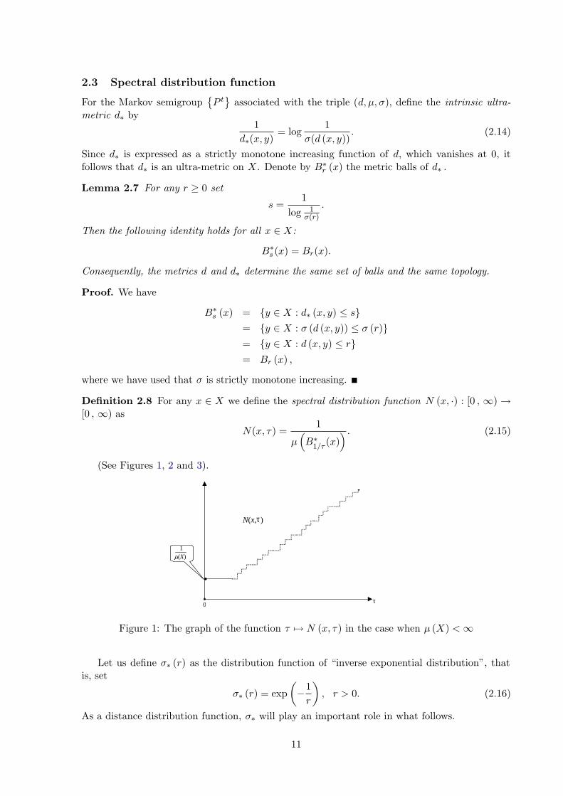
Definition 2.8 For any x ∈ X we define the spectral distribution function N (x, ∙) : [0 , ∞) →[0 , ∞) as

N(x, τ ) =1

μ(B∗

1/τ (x)) . (2.15)

(See Figures 1, 2 and 3).

0 τ

N(x, )

μ(X) 1

τ

Figure 1: The graph of the function τ 7→ N (x, τ ) in the case when μ (X) < ∞

Let us define σ∗ (r) as the distribution function of “inverse exponential distribution”, thatis, set

σ∗ (r) = exp

(

−1r

)

, r > 0. (2.16)

As a distance distribution function, σ∗ will play an important role in what follows.

11

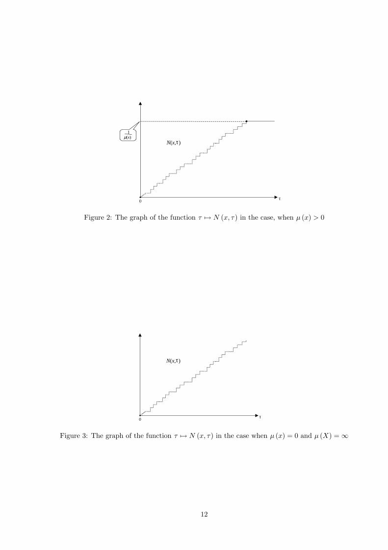
0 τ

N(x, ) μ(x)

1

τ

Figure 2: The graph of the function τ 7→ N (x, τ ) in the case, when μ (x) > 0

0 τ

N(x, ) τ

Figure 3: The graph of the function τ 7→ N (x, τ ) in the case when μ (x) = 0 and μ (X) = ∞

12

Definition 2.9 An isotropic Markov operator P associated with a triple (d, μ, σ∗) will be re-ferred to as a standard Markov operator, associated with (d, μ).

Theorem 2.10 Let d∗ and σ∗ be defined by (2.14) and (2.16).

(a) The triples (d, μ, σ) and (d∗, μ, σ∗) induce the same isotropic Markov operators.

(b) The heat kernel p (t, x, y) associated with the triple (d, μ, σ) satisfies for all x, y ∈ X andt > 0 the following identities:

p(t, x, y) =∫ t/d∗(x,y)

0N(x,

s

t

)e−sds (2.17)

and

p(t, x, y) = t

∫ 1/d∗(x,y)

0N(x, τ ) exp(−τt) dτ. (2.18)

Consequently, p (t, x, y) is a finite continuous function of t, x, y for all t > 0 and x 6= y.

As it follows from (a), any isotropic Markov operator is at the same time the standardMarkov operator, associated with (d∗, μ).Proof. (a) It suffices to show that

p (t, x, y) =∫

[d∗(x,y),∞)

dσt∗ (u)

μ (B∗u (x))

, (2.19)

where by Theorem 2.2 the right hand side represents the heat kernel associated with the triple(d∗, μ, σ∗). Consider the function

u (r) =1

log 1σ(r)

, r ∈ [0,∞)

and observe that

1. u (d (x, y)) = d∗ (x, y), u (∞) = ∞;

2. σ∗ (u (r)) = exp(− 1

u(r)

)= σ (r) ;

3. B∗u(r) (x) = Br (x) by Lemma 2.7.

Making the change u = u (r) in the integral in (2.19), we obtain∫

[d∗(x,y),∞)

dσt∗ (u)

μ (B∗u (x))

=∫

[d(x,y),∞)

dσt (r)μ (Br (x))

,

which together with (2.8) implies (2.19). Clearly, (2.20) follows from (2.17) as d∗ (x, x) = 0.

(b) The change s = t/u in (2.19) yields

p (t, x, y) =∫

[d∗(x,y),∞)

d exp(− t

u

)

μ (B∗u (x))

=∫ 0

t/d∗(x,y)

de−s

μ(B∗

t/s (x))

=∫ t/d∗(x,y)

0N(x,

s

t

)e−sds

13

which proves (2.17). Another change s = tτ transforms (2.17) to (2.18).

In the case x = y we obtain from (2.17) and (2.18)

p(t, x, x) =∫ ∞

0N(x,

s

t

)e−sds = t

∫ ∞

0N(x, τ ) exp(−τt) dτ. (2.20)

Depending on the function N (x, τ ), the on-diagonal value p (t, x, x) can be equal to ∞. For anyx ∈ X set

T (x) := lim supτ→∞

log N(x, τ )τ

. (2.21)

Corollary 2.11 The function t 7→ p (t, x, x) is monotone decreasing and p(t, x, x) < ∞ forall t > T (x) .

Proof. The monotonicity of p (t, x, x) follows from the first identity in (2.20), while the secondclaim follows from the second identity in (2.20). Observe also that if limτ→∞

log N(x,τ)τ exists

and hence is equal to T (x) then p (t, x, x) = ∞ for t < T (x).

Proposition 2.12 Assume that T (x) < ∞ for some x ∈ X.

(a) For all y ∈ X,

limt→∞

p(t, x, y) =1

μ(X),

where the convergence is locally uniform in y ∈ X.

(b) For all y ∈ X,

limt→∞

p(t, x, y)p(t, x, x)

= 1,

where the convergence is locally uniform in y ∈ X.

Proof. (a) As t → ∞ we have

N(x,

s

t

)→ N (x, 0) =

1μ (X)

and t/d∗ (x, y) → ∞. Hence, we obtain from (2.17)

limt→∞

p (t, x, y) =∫ ∞

0

1μ (X)

e−sds =1

μ (X),

provided we justify that the integral and lim are interchangeable. The latter follows from thedominated convergence theorem, because the hypothesis T (x) < ∞ implies that, for someA, a > 0 and all τ > 0,

N (x, τ ) ≤ A exp (aτ) (2.22)

whence

N(x,

s

t

)e−s ≤ A exp

((a

t− 1)

s)≤ A exp

(

−12s

)

(2.23)

for t > 2a, so that the domination condition is satisfied.

(b) Set r = d∗ (x, y). It follows from (2.17) and (2.20) that

p (t, x, x) − p (t, x, y) =∫ ∞

t/rN(x,

s

t

)e−sds.

14

Assuming t > 2a and applying (2.23), we obtain

p (t, x, x) − p (t, x, y) ≤ A

∫ ∞

t/re−

12sds = 2A exp

(

−t

2r

)

,

whereas

p(t, x, x) ≥∫ ∞

t4r

N(x,

s

t

)e−sds ≥ N

(

x,14r

)

exp

(

−t

4r

)

.

It follows thatp(t, x, x) − p(t, x, y)

p(t, x, x)≤

2A exp(− t

4r

)

N(x, 1

4r

) → 0 as t → ∞.

2.4 Estimates of the heat kernel

The purpose of this section is to provide some estimates of the isotropic heat kernel. Recall thatby Theorem 2.10

p(t, x, y) =∫ t/d∗(x,y)

0N(x,

s

t

)e−sds. (2.24)

Definition 2.13 A monotone increasing function Φ : R+ → R+ is said to satisfy the doublingproperty if there exists a constant D > 0 such that

Φ(2s) ≤ DΦ(s) for all s > 0.

It is known (Potter’s theorem) that if Φ is doubling then

Φ(s2) ≤ D

(s2

s1

)γ

Φ(s1) for all 0 < s1 < s2 , where γ = log2 D. (2.25)

Theorem 2.14 Suppose that, for some x ∈ X, the function τ 7→ N(x, τ ) is doubling. Then

c t

t + d∗(x, y)N

(

x,1

t + d∗(x, y)

)

≤ p(t, x, y) ≤C t

t + d∗(x, y)N

(

x,1

t + d∗(x, y)

)

(2.26)

for all t > 0, y ∈ X and some constants C, c > 0 depending on the doubling constant.

In what follows we will use the relation f ' g between two positive function f, g, whichmeans that the ratio f/g is bounded from above and below by positive constants, for a specifiedrange of the variables. In particular, we can write (2.26) shortly in the form

p (t, x, y) 't

t + d∗(x, y)N

(

x,1

t + d∗(x, y)

)

(2.27)

for a fixed x and all y ∈ X, t > 0.

Example 2.15 Assume that, for some x ∈ X and α > 0,

N (x, τ ) ' τα for all τ > 0.

Then by (2.27)

p(t, x, y) 't

(t + d∗(x, y))1+α 't

(t2 + d∗(x, y)2)1+α

2

,

that is, p (t, x, y) behaves like the Cauchy distribution in “α-dimensional” space.

15

Example 2.16 More generally, assume that, for some α, β ≥ 0,

N(x, τ ) '

{τα, 0 < τ ≤ 1,τβ , τ > 1.

(2.28)

Then we obtain by (2.27)

p(t, x, y) '

t

(t + d∗(x, y))1+β, t + d∗(x, y) ≤ 1,

t

(t + d∗(x, y))1+α , t + d∗(x, y) > 1.(2.29)

For example, let X be a discrete locally finite group, like X =⊕∞

k=1 Z (nk), and μ be theHaar measure, normalized to μ (x) = 1. With the discrete ultra-metric we obtain by (2.15) thatN (x, τ ) ' 1 for large enough τ . Assuming additionally that

N (x, τ ) ' τα for small τ,

we see that (2.28) and, hence, (2.29) hold with β = 0 (cf. [13]).

Example 2.17 Assume that τ 7→ N (x, τ ) is doubling and, for some α > 0,

N (x, τ ) '

(

log1τ

)−α

for τ <12.

Then by (2.27)

p (t, x, y) 't

(t + d∗(x, y)) logα (t + d∗ (x, y))

provided t + d∗ (x, y) > 2.

Example 2.18 Assume that, for some α > 0,

N (x, τ ) ' exp(−τ−α

).

In this case Theorem 2.14 does not apply. An ad hoc method of estimating the integral in (2.24)yields in this case

p (t, x, y) ≤C3t

t + d∗ (x, y)exp

(−c3

(t

αα+1 + d∗ (x, y)α

))

and

p (t, x, y) ≥C4t

t + d∗ (x, y)exp

(−c4

(t

αα+1 + d∗ (x, y)α

)),

for all x, y ∈ X, t > 0 and some positive constants C3,C4, c3, c4.

For the proof of Theorem 2.14 we need a sequence of lemmas.

Lemma 2.19 For all x, y ∈ X and t > 0 the following estimates hold.

(a)

p(t, x, y) ≤t

d∗(x, y)N

(

x,1

d∗(x, y)

)

. (2.30)

16

(b)

p(t, x, y) ≥12e

t

d∗(x, y)N

(

x,1

2d∗(x, y)

)

, t ≤ d∗ (x, y) ,

N

(

x,12t

)

, t ≥ d∗ (x, y) .

(2.31)

(c)

p(t, x, x) ≥1eN

(

x,1t

)

. (2.32)

Proof. (a) Inequality (2.30) follows from (2.24) using the monotonicity of τ 7→ N (x, τ ) thatyields

N(x,

s

t

)e−s ≤ N

(

x,1

d∗ (x, y)

)

.

(b) Set a = min(1, t

d∗(x,y)

). It follows from (2.24) that

p(t, x, y) ≥∫ a

a/2N(x,

s

t)e−s ds ≥ N

(x,

a

2t

) a

2e,

which is equivalent to (2.31).

(c) We have by (2.20)

p(t, x, x) ≥∫ ∞

1N(x,

s

t)e−sds ≥ N

(

x,1t

)∫ ∞

1e−sds,

whence (2.32) follows.

Lemma 2.20 The following inequalities hold for all x, y ∈ X and t > 0:

p(t, x, y) ≥12e

t

t + d∗(x, y)N

(

x,1

2 (t + d∗(x, y))

)

, (2.33)

and

p(t, x, y) ≤ 2et

t + d∗(x, y)p

(t + d∗(x, y)

2, x, x

)

. (2.34)

Proof. The lower bound (2.33) follows immediately from (2.31). To prove (2.34), observe thatby (2.30) and (2.32)

p (t, x, y) ≤ et

d∗ (x, y)p (d∗ (x, y) , x, x) ,

which yields (2.34) in the case t ≤ d∗ (x, y) as the function p (∙, x, x) is monotone decreasing. Inthe case t > d∗ (x, y) (2.34) follows trivially from (2.12), that is, from

p (t, x, y) ≤ p (t, x, x) ,

using again the monotonicity of p (∙, x, x).

Lemma 2.21 For any given x ∈ X, the following two properties are equivalent.

(i) For some constant C and all t > 0,

p(t, x, x) ≤ CN

(

x,1t

)

. (2.35)

17

(ii) The function τ 7→ N(x, τ ) is doubling, that is, for some constant D,

N (x, 2τ) ≤ DN (x, τ.)

Proof. (ii) ⇒ (i). The estimate (2.35) follows from (2.20) and (2.25) as follows:

p(t, x, x) = N

(

x,1t

)∫ ∞

0

N(x, s

t

)

N(x, 1

t

)e−sds

≤ DN

(

x,1t

)∫ ∞

0max{1, sγ}e−sds

= CN

(

x,1t

)

.

(i) ⇒ (ii). The upper bound (2.35) implies, for any t > 0,

CN

(

x,1t

)

≥ p(t, x, x) ≥∫ ∞

2N(x,

s

t)e−sds

≥ e−2 N

(

x,2t

)

,

whence the doubling property of N (x, ∙) follows.

Proof of Theorem 2.14. The lower bound in (2.26) follows from (2.33), the upper boundfollows from (2.34) and (2.35).

In conclusion of this section we provide practicable conditions for the validity of the doublingproperty of N (x, ∙).

Definition 2.22 A monotone increasing function Ψ : R+ → R+ is said to satisfy the reversedoubling property, if there is a constant δ ∈ (0, 1) such that for all r > 0

Ψ(r) ≥ 2Ψ(δr).

Proposition 2.23 Fix some x ∈ X. The function τ 7→ N(x, τ ) is doubling provided the follow-ing two conditions hold:

(i) The function Ψ(r) = −1/ log σ(r) satisfies the reverse doubling property.

(ii) The volume function r 7→ μ (Br(x)) satisfies the doubling property.

Proof. We use the following short notation for the balls centered at x: Br = Br (x) and B∗r =

B∗r (x). It follows from the Definition 2.8 of the spectral distribution function that τ 7→ N(x, τ )

is doubling if and only if the function s 7→ μ(B∗s ) is doubling. Set Φ = Ψ−1 and observe that the

reverse doubling property for Ψ is equivalent to the doubling property for Φ. By Lemma 2.7 wehave B∗

Ψ(r) = Br which implies that B∗s = BΦ(s). Using the hypotheses (ii) and (2.25) for the

function μ (Br), we obtain

μ (B∗2s) = μ

(BΦ(2s)

)≤ D

(Φ(2s)Φ (s)

)γ

μ(BΦ(s)

)≤ const μ (B∗

s ) ,

which was to be proved.

18

2.5 Heat kernels in Qp

Given a prime p, the p-adic norm on Q is defined as follows: if x = pn ab , where a, b are integers

not divisible by p, then‖x‖p := p−n.

If x = 0 then ‖x‖p := 0. The p-adic norm on Q satisfies the ultra-metric inequality. Indeed, ify = pm c

d and m ≤ n then

x + y = pm

(pn−ma

b+

c

d

)

whence‖x + y‖p ≤ p−m = max

{‖x‖p , ‖y‖p

}.

Hence, Q with the metric d (x, y) = ‖x − y‖p is an ultra-metric space, and so is its completionQp – the field of p-adic numbers.

Every p-adic number x has a representation

x =∞∑

k=−N

akpk = ...ak...a2a1a0∙a−1a−2...a−N (2.36)

where N ∈ N and ak ∈ {0, . . . , p − 1} are p-adic digits. The rational number 0.a−1...a−N =∑k=−1k=−N akp

k is called the fractional part of x and the rest∑∞

k=0 akpk is the integer part of x.

For any n ∈ Z, the d-ball Bp−n (x) consists of all numbers

y =∞∑

k=−N

bkpk = ...bk...b2b1b0∙b−1b−2...b−N

such that bk are arbitrary for k ≥ n and bk = ak for k < n. It follows that Bp−n (x) decomposesinto a disjoint union of p balls of radii p−(n+1) depending on the choice of bn.

For example, B1 (0) coincides with the set Zp of all p-adic integers, that is, any y ∈ B1 (0)has the form

y = ...bk...b2b1b0

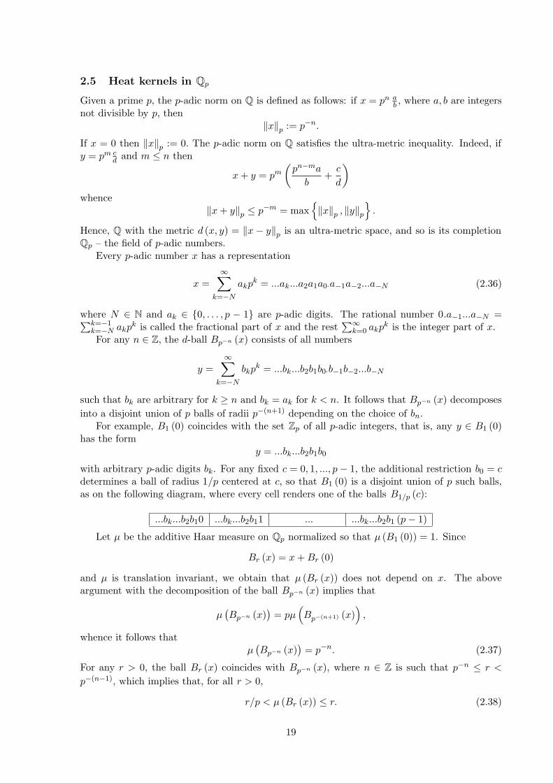
with arbitrary p-adic digits bk. For any fixed c = 0, 1, ..., p − 1, the additional restriction b0 = cdetermines a ball of radius 1/p centered at c, so that B1 (0) is a disjoint union of p such balls,as on the following diagram, where every cell renders one of the balls B1/p (c):

...bk...b2b10 ...bk...b2b11 ... ...bk...b2b1 (p − 1)

Let μ be the additive Haar measure on Qp normalized so that μ (B1 (0)) = 1. Since

Br (x) = x + Br (0)

and μ is translation invariant, we obtain that μ (Br (x)) does not depend on x. The aboveargument with the decomposition of the ball Bp−n (x) implies that

μ(Bp−n (x)

)= pμ

(Bp−(n+1) (x)

),

whence it follows thatμ(Bp−n (x)

)= p−n. (2.37)

For any r > 0, the ball Br (x) coincides with Bp−n (x), where n ∈ Z is such that p−n ≤ r <

p−(n−1), which implies that, for all r > 0,

r/p < μ (Br (x)) ≤ r. (2.38)

19

Example 2.24 Let (X, d, μ) be Qp with p-adic distance and the Haar measure μ. Consider thedistance distribution function

σ(r) = exp (−(b/r)α) ,

where α, b > 0. Since

Ψ(r) :=1

log 1σ(r)

= (r/b)α ,

we obtain by (2.14)

d∗(x, y) = Ψ (d (x, y)) =

(‖x − y‖p

b

)α

. (2.39)

By Lemma 2.7, we haveB∗

s (x) = BΨ−1(s) (x) ,

which together with (2.38) yields

μ (B∗s (x)) ' s1/α . (2.40)

Consequently, we obtainN(x, τ ) ' τ1/α.

Since this function is doubling, Theorem 2.14 (cf. also Example 2.15) yields the estimate

p(t, x, y) 't

(t + d∗(x, y))1+1/α'

t

(t1/α + ‖x − y‖p)1+α

.

In particular, for all t > 0 and x ∈ X

p (t, x, x) ' t1/α.

Example 2.25 Let X = Zp, that is, X is the unit ball B1 (0) in Qp, with the p-adic distanceand the Haar measure μ. Consider the distance distribution function

σ (r) = exp(1 − exp r−α

),

for some α > 0. Since for r ≤ 1

Ψ(r) :=1

log 1σ(r)

=1

exp r−α − 1' exp

(−r−α

),

we obtain thatd∗(x, y) = Ψ (d (x, y)) ' exp

(−‖x − y‖−α

p

).

By Lemma 2.7 and (2.38), we have, for all s ≤ 12 ,

μ (B∗s (x)) = μ

(BΨ−1(s) (x)

)' Ψ−1 (s) '

1

log1/α 1s

,

whereas for s > 12 we have μ (B∗

s (x)) ' 1. Therefore, we obtain, for all τ > 0,

N (x, τ ) =1

μ(B∗

1/τ (x)) ' log1/α (2 + τ) .

Hence, the function N (x, τ ) is doubling, and we obtain by (2.27) that

p(t, x, y) 't

t + exp(−‖x − y‖−α

p

) log1/α

2 +1

t + exp(−‖x − y‖−α

p

)

.

20

Example 2.26 Let X be the subset of Qp consisting of all p-adic fractions, that is, the numbersof the form x = 0.a−1....a−N . Then the p-adic distance d on X takes only integer values so that(X, d) is a discrete space. Let μ be the counting measure on X, that is, μ (x) = 1 for any x ∈ X.Consider the following distance distribution function

σ (r) = exp

(

−1

logα (2r)

)

for r ≥ 1, (2.41)

that is arbitrarily extended to r < 1 to be strictly monotone increasing and to have σ (0) = 0.Since

Ψ(r) :=1

log 1σ(r)

= logα (2r) for r ≥ 1,

we obtain, for x 6= y,

d∗(x, y) = Ψ (d (x, y)) = logα(2 ‖x − y‖p

). (2.42)

For s ≥ s0 := logα 2, we have

μ (B∗s (x)) = μ

(BΨ−1(s) (x)

)' Ψ−1 (s) =

12

exp(s1/α

), (2.43)

whereas for s < s0 we have μ (B∗s (x)) ' μ (x) = 1. We see that (2.43) holds for all s > 0. It

follows that, for all τ > 0,

N (x, τ ) =1

μ(B∗

1/τ (x)) ' exp

(−τ−1/α

). (2.44)

By Example 2.18, we obtain

p (t, x, y) ≤Ct

t + logα+

(2 ‖x − y‖p

) exp(−c(t

1α+1 + log+

(2 ‖x − y‖p

))),

and a similar lower bound.

2.6 Green function and transience

Given an isotropic heat semigroup{P t}, define the Green operator G on non-negative Borel

functions f on X by

Gf (x) =∫ ∞

0P tf (x) dt.

Of course, the value of Gf (x) could be ∞. By Fubini’s theorem, we obtain

Gf (x) =∫

Xg (x, y) f (y) dμ (y)

where

g (x, y) =∫ ∞

0p (t, x, y) dt.

Substituting the heat kernel from (2.18) and using again Fubini’s theorem, we obtain

g(x, y) =∫ 1/d∗(x,y)

0

N(x, τ ) dτ

τ2=∫ ∞

d∗(x,y)

ds

μ (B∗s (x))

, (2.45)

where the second identity follows from (2.15). The function g (x, y) is called the Green functionof the semigroup

{P t}. Note that the Green function can be identically equal to ∞. For

example, this is the case when μ (X) < ∞ (cf. Figure 1) and the second integral (2.45) divergesat ∞.

21

Definition 2.27 The process {Xt} and the semigroup {P t} are called transient if Gf is abounded function whenever f is bounded and has compact support, and recurrent otherwise.

Theorem 2.28 The following statements are equivalent.

(i) The semigroup {P t} is transient.

(ii) g(x, y) < ∞ for some/all distinct x, y ∈ X.

(iii) For some/all x ∈ X, ∫ ∞ ds

μ (B∗s (x))

< ∞. (2.46)

The inequality (2.46) is equivalent to∫

0

N(x, τ ) dτ

τ2< ∞ . (2.47)

Observe that, in the transient case, the function x, y 7→ 1g(x,y) determines an ultra-metric on X,

which is proved similarly to Corollary 2.6.Proof. The validity of the condition (2.46) is independent of the choice of x because for anytwo x, x′ ∈ X the balls B∗

s (x) and B∗s (x′) are identical provided s ≥ d (x, x′). The finiteness

of the second integral in (2.45) for x 6= y is clearly equivalent to (2.46), whence the equivalence(ii) ⇔ (iii) follows, with all combinations of some/all options.

The finiteness of Gf for any bounded function f with compact support clearly implies thatg (x, y) 6≡ ∞, that is, (i) ⇒ (ii). So, it remains to prove (iii) ⇒ (i). It suffices to show that Gfis bounded for f = 1A where A is a bounded Borel subset of X. Let R be the diameter of Awith respect to the distance d∗. Then we have A ⊂ B∗

R (x) for any x ∈ A whence by (2.45)

Gf (x) =∫

Ag (x, y) dμ (y) ≤

∫

B∗R(x)

g (x, y) dμ (y)

=∫

B∗R(x)

∫ ∞

01[d∗(x,y),∞) (s)

ds

μ (B∗s (x))

dμ (y)

=∫ ∞

0

1μ (B∗

s (x))

(∫

B∗R(x)

1[0,s] (d∗ (x, y)) dμ (y)

)

ds

=∫ ∞

0

1μ (B∗

s (x))μ (B∗

R (x) ∩ B∗s (x)) ds.

For s ≥ R the integrand is equal to 1μ(B∗

s (x))μ (B∗R (x)) so that the convergence at ∞ follows

from (2.46). The convergence is clearly uniform in x ∈ A because μ (B∗R (x)) and μ (B∗

s (x)) areindependent of x ∈ A for s ≥ R. For s ≤ R the integrand is equal to

1μ (B∗

s (x))μ (B∗

s (x)) = 1,

whence the uniform convergence at 0 follows. Hence, supA Gf (x) < ∞. That supX Gf (x) < ∞follows from the decay of g (x, y) in d∗ (x, y).

Let us note that if X is a locally finite group with the Haar measure μ, then the transiencecriterion (iii) of Theorem 2.28 coincides with the general sufficient condition of transience of[40].

Now let us provide some estimate of the Green function. Set

V (x, r) = μ (B∗r (x)) . (2.48)

22

Theorem 2.29 Assume that there exist constants 1 < c < c′ < c′′ such that for all r > r0 ≥ 0and some x ∈ X

c′ ≤V (x, cr)V (x, r)

≤ c′′. (2.49)

Then the semigroup{P t}

is transient and, for all y ∈ X such that r := d∗ (x, y) > r0, we have

g (x, y) 'r

V (x, r).

Note that the condition V (x,cr)V (x,r) ≤ c′′ is equivalent to the doubling property of r 7→ V (x, r)

(cf. Definition 2.13), whereas the condition V (x,cr)V (x,r) ≥ c′ with c′ > c is somewhat stronger than

the reverse doubling property (cf. Definition 2.22). For example, (2.49) holds for V (x, r) ' rα

if and only if α > 1.Proof. Set for simplicity of notation V (s) := V (x, s). For r > r0 we have

g (x, y) =∫ ∞

r

ds

V (s)=

∞∑

k=0

∫ ck+1r

ckr

ds

V (s)=

∞∑

k=0

ck

∫ cr

r

ds

V (cks)

Using the lower bound in (2.49), we obtain

∫ ∞

r

ds

V (s)≤

∞∑

k=0

ck

∫ cr

r

(c′)−k ds

V (s)≤

∞∑

k=0

( c

c′

)k cr

V (r)≤ const

r

V (r),

where the series converges due to c′ > c. Similarly, using the upper bound in (2.49), we obtain

∫ ∞

r

ds

V (s)≥∫ cr

r

ds

V (s)≥

(c − 1) r

V (cr)≥ const

r

V (r),

which finishes the proof.

Example 2.30 Let (X, d, μ) and σ be as in Example 2.24, that is, X = Qp is the field of p-adicnumbers with ultra-metric d(x, y) = ‖x − y‖p and σ(r) = exp (−(b/r)α). Then by (2.39) wehave

d∗ (x, y) = const ‖x − y‖αp

and by (2.40)V (x, r) ' r1/α.

Therefore, by Theorem 2.28, the semigroup {P t} is transient if and only if α < 1. Moreover, thecondition (2.49) is fulfilled also if and only if α < 1, and in this case we obtain by Theorem 2.29that, for all x, y,

g(x, y) ' d∗ (x, y)1−1α ' ‖x − y‖α−1

p .

Example 2.31 Let (X, d, μ) and σ be as in Example 2.26, that is, X is the set of fractionalp-adic numbers and σ is given by (2.41). By (2.42) we have, for x 6= y,

d∗(x, y) = logα(2 ‖x − y‖p

)

and by (2.43)

V (x, r) ' exp(r1/α

).

23

By Theorem 2.28 we conclude that the semigroup{P t}

is transient. Theorem 2.29 does notapply in this case, but a direct estimate of the integral in (2.45) yields, for r := d∗ (x, y) ,

g (x, y) =∫ ∞

r

ds

V (x, s)'∫ ∞

rexp

(−s1/α

)ds ' r1−1/α exp

(−r1/α

),

whence, for x 6= y,

g (x, y) ' ‖x − y‖−1p logα−1

(2 ‖x − y‖p

).

3 Isotropic Laplacian and its spectrum

In this section we are concerned with the properties of the generator of the isotropic semigroup{P t}. By definition, the generator L of a strongly continuous semigroup {Pt}t≥0 in a Banach

space is defined by

Lf = s- limt→0

f − Ptf

t

and the domain domL consists of those f for which the above limit exists. Since the isotropicsemigroup

{P t}

is symmetric and acts in a Hilbert space L2 (X,μ), the above definition isequivalent to the following: L is a self-adjoint (unbounded) operator in L2 (X,μ) such that

P t = exp (−tL) for all t > 0.

Obviously, this is equivalent to P = exp (−L), which leads to the identity

L = log1P

,

where the right hand side is understood in the sense of functional calculus of self-adjoint oper-ators. We refer to L as an isotropic Laplace operator associated with (d, μ, σ).

3.1 Subordination

Using the spectral decomposition (2.10) of P , we obtain that

L =∫

[0,+∞)log

1σ (1/λ)

dEλ

where {Eλ} is the spectral resolution defined by (2.6). Denote for simplicity

ϕ (λ) := log1

σ (1/λ)(3.1)

so that

L =∫

[0,+∞)ϕ (λ) dEλ . (3.2)

The domain domL is then given by

domL =

{

f ∈ L2 :∫ ∞

0ϕ (λ)2 d (Eλf, f) < ∞

}

.

Observe that the function ϕ has the following properties that follow from the assumptions (1.5)about σ:

ϕ : [0,∞] → [0,∞] is a strictly monotone increasingright-continuous function, such that ϕ (0) = 0 and ϕ (∞−) = ∞.

(3.3)

24

Conversely, any function ϕ satisfying (3.3) determines the function

σ (λ) = exp (−ϕ (1/λ))

that satisfies (1.5). This observation leads us to the following interesting subordination propertyof isotropic Laplacians.

Theorem 3.1 Let L be an isotropic Laplacian associated with (d, μ, σ). Let ψ be any functionsatisfying (3.3). Then ψ (L) is also an isotropic Laplacian associated with (d, μ, σ) for someother distance distribution function σ.

Proof. It follows from (3.2) that

ψ (L) =∫

[0,+∞)ψ ◦ ϕ (λ) dEλ.

Since the composition ψ ◦ ϕ also satisfies (3.3), we obtain that ψ (L) is an isotropic Laplacian.Moreover, using (3.1), we obtain the following formula for σ:

σ (r) = exp

(

−ψ

(

log1

σ (r)

))

.

Remark 3.2 Any a non-negative definite, self-adjoint operator L in L2 generates a semigroup{e−tL

}t≥0

. We refers to L as a Laplacian if the semigroup{e−tL

}is Markovian. In general, by

Bochner’s theorem, for any Laplacian L, the operator ψ(L) is again a Laplacian, provided ψ isa Bernstein function (see, for example, Schilling, Song and Vondracek [53]). It is known thatψ(λ) = λα is a Bernstein function if and only if 0 < α ≤ 1. Thus, for a general Laplacian L,the power Lα is guaranteed a Laplacian only for α ≤ 1. For example, for the classical Laplaceoperator L = −Δ in Rn, the power (−Δ)α with α > 1 is not a Laplacian. In a striking contrastto that, by Theorem 3.1, the powers Lα of the isotropic Laplacian are again Laplacians for allα > 0.

3.2 L2-spectrum

Our next goal is to give an explicit expression for Lf and to describe the spectrum of L. Recallthat by Theorem 2.10 the triples (d, μ, σ) and (d∗, μ, σ∗) induce the same Markov operator Pand, hence, the same Laplace operator L, where d∗ is the intrinsic ultra-metric defined by (2.14)and

σ∗ (r) = exp

(

−1r

)

From now on we will use only the metric d∗ and σ∗. Let the spectral resolution {Eλ} be alsodefined using the metric d∗, which means that in the definition (2.6) of Eλ we now use theaveraging operator Qr with respect to the metric d∗. The function ϕ∗ associated with σ∗ by(3.1) has especially simple form: ϕ∗ (λ) = λ. Therefore, we obtain from (3.2) the spectraldecomposition of L in the classical form

L =∫

[0,+∞)λdEλ =

∫

(0,∞)λdEλ. (3.4)

The change s = 1λ gives

L = −∫

(0,∞)

1sdQs.

25

For any x ∈ X, denote by Λ (x) the set of values of d∗ (x, y) for all y ∈ X, y 6= x, that is,

Λ (x) = {d (x, y) : y ∈ X \ {x}} . (3.5)

Lemma 3.3 The set Λ (x) has no accumulation point in (0,∞). Consequently, Λ (x) is at mostcountable.

Proof. Let r ∈ (0,∞) be an accumulation point of Λ (x), that is, there is a sequence {rk} fromΛ (x) \ {r} such that rk → r as k → ∞. Then rk = d∗ (x, yk) for some yk ∈ X. Since thesequence {yk} is bounded, by the compactness of all balls in X it has a convergent subsequence.Without loss of generality, we can then assume that {yk} converges, say to y ∈ X. Then wehave r = d (x, y). Since r > 0, we have for large enough k that rk > r/2 and d (y, yk) < r/2.Then we obtain by the ultra-metric inequality that

rk ≤ max (r, d (y, yk)) = r

and analogouslyr ≤ max (rk, d (y, yk)) = rk

whence rk = r, which contradicts the assumptions.

Definition 3.4 For any ball B in X denote by ρ (B) the minimal d∗-radius of B.

Note that ρ (B) exists because all balls are defined as closed balls, and ρ (B) coincides withthe d∗-diameter of B.

Lemma 3.5 If ρ (B) > 0 then ρ (B) ∈ Λ (x) for any x ∈ B. Conversely, any number in Λ (x)is equal to ρ (B) for some ball B containing x.

Proof. Set r = ρ (B) so that B = B∗r (x). For any y ∈ B we have d∗ (x, y) ≤ r, and we have

to show that d∗ (x, y) = r for some y. Assume that d∗ (x, y) < r for all y ∈ B. Then the set{d∗ (x, y) : y ∈ B \ {x}} is a subset of (0, r)∩Λ (x). By Lemma 3.3, the latter set has a maximalelement, say r′. Then B ⊂ B∗

r′ (x), which contradicts the minimality of radius r. Conversely, ifr ∈ Λ (x) then the ball B = Br (x) has ρ (B) = r since there exists y ∈ X with d (x, y) = r.

Definition 3.6 Let B,C be two balls in X such that C ⊂ B. We say that C is a child orsuccessor of B (and B is a parent or predecessor of C) if C 6= B and, for any ball A, such thatC ⊂ A ⊂ B we have A = C or A = B. In other words, B is a minimal ball containing C as aproper subset. If C is a child of B then we write C ≺ B.

Denote by K be the family of all balls C in X with positive radii. If C = B∗r (x) is a ball

from K with r > 0 then for the minimal radius ρ (C) we have two possibilities:

1. either ρ (C) > 0,

2. or ρ (C) = 0 and the center of C is an isolated point of X.

Lemma 3.7 For any ball C ∈ K such that C 6= X there is a unique parent ball B. For any ballB with ρ (B) > 0 the number deg (B) of its children satisfies 2 ≤ deg (B) < ∞. Moreover, allthe children of B are disjoint and their union is equal to B.

26

Proof. Fix some x ∈ C. It follows from Lemma 3.3 and the definition of K that the set(ρ (C) ,∞) ∩ Λ (x) has a minimum that we denote by r. Then the ball B∗

r (x) is a parent of C.The uniqueness of the parent follows from definition.

If C1 and C2 are two distinct children of B then C1 and C2 are disjoint. Indeed, if theyintersect then one of them contains the other, say C1 ⊂ C2. By definition of a parent/child, wemust have then C2 = C1 or C2 = B, whence C1 = C2 follows.

Let us show that for any x ∈ B there is a ball C such that x ∈ C ≺ B. Indeed, if the set(0, ρ (B)) ∩ Λ (x) is empty, then C = B∗

0 (x) = {x} is the child of B. If the set (0, ρ (B)) ∩ Λ (x)is non-empty then by Lemma 3.3 is has a maximum, say r. Then C = B∗

r (x) is a child of B.Hence, the set of all children of B is a covering of B.

Each child C of B is an open set (being also a closed ball) because C coincides with an openball of radius ρ (B). Since B is compact, it follows that the set of its children is finite, that is,deg (B) < ∞. Finally, deg (B) cannot be equal to 1 since then B would coincide with its onlychild. Hence, deg (B) ≥ 2.

For any C ∈ K define the function fC on X as follows. If C is a proper subset of X then,denoting by B the parent of C, set

fC =1

μ(C)1C −

1μ(B)

1B (3.6)

(note that always μ (C) > 0). Set also λ (C) := 1/ρ (B). If C = X (which can only be the casewhen X is compact), then set fC ≡ 1 and λ (C) = 0.

Theorem 3.8 For any C ∈ K the function fC is an eigenfunction of L with the eigenvalueλ (C). The family {fC : C ∈ K} is complete (its linear span is dense) in L2 (X,μ) . Consequently,the operator L has a complete system of compactly supported eigenfunctions.

Proof. Fix a ball C ∈ K or radius r = ρ (C), and let B be the parent of radius r′ = ρ (B).Any ball of radius s < r′ either is disjoint with C or is contained in C, which implies that 1C

is constant in any such ball. It follows that, for any s < r′, we have Qs1C = 1C and, similarlyQs1B = 1B , whence

QsfC = fC .

For s ≥ r′ any ball of radius s either contains both balls C,B or is disjoint from B. Since theaverages of the two functions 1

μ(C)1C and 1μ(B)1B over any ball containing C and B are equal,

we obtain that in this case QsfC = 0. It follows that

LfC = −∫

(0,∞)

1sQsfC ds =

1r′

fC = λ (C) fC ,

which proves that fC is an eigenfunction of L with the eigenvalue λ (C). In the case of compactX we have QsfX = fX for all s > 0, whence LfX = 0 = λ (X).

Let us show that the system {fC : C ∈ K} is complete. We assume that some function f ∈ L2

is orthogonal to all functions fC and prove that f ≡ const . We have for any r > 0,

(Qrf, fC)L2 = (f, QrfC)L2 = const (f, fC)L2 = 0,

where we have used the fact that any eigenfunction of L is also eigenfunction of Qr with aneigenvalue that we denoted by const. Hence, Qrf is also orthogonal to all fC . We will provebelow that Qrf = 0, which will imply by (2.2) that f = 0.

Since Qrf is constant in any ball of radius r, by renaming Qrf back to f we can assumefrom now on that f is constant in any ball of radius r. Fix some ball C ∈ K and its parent B.It follows from (3.6) that (f, fC)L2 = 0 is equivalent to

1μ(C)

∫

Cf dμ =

1μ(B)

∫

Bf dμ,

27

that is, the average value of f over a ball is preserved when switching to its parent. Startingwith two balls C1 and C2 of radii r, we can build a sequence of their predecessors which endup with the same (large enough) ball. This implies that the averages of f in C1 and C2 are thesame. Since f is constant in C1 and C2, it follows that the values of these constants are thesame. It follows that f ≡ const on X. If μ (X) = ∞ then we obtain f ≡ 0. If μ (X) < ∞ thenusing the orthogonality of f to fX ≡ 1 we obtain again that f ≡ 0.

For any ball B with ρ (B) > 0 define the subspace HB of L2 as follows:

HB = span{fC : C ≺ B}. (3.7)

By Theorem 3.8, all non-zero functions in HB are the eigenfunctions of L with eigenvalue 1ρ(B) .

It follows from Lemma 3.7 that the functions {1C : C ≺ B} are linearly independent and

∑

C≺B

1C = 1B .

This entails ∑

C≺B

μ(C)fC = 0 (3.8)

and that this is the only dependence between functions fC . Hence, we obtain that

dimHB = deg (B) − 1. (3.9)

Clearly, the spaces HB and HB′ are orthogonal provided the balls B,B′ are disjoint.Define the set

Λ := {d∗ (x, y) : x, y ∈ X, x 6= y} =⋃

x∈X

Λ (x) . (3.10)

Theorem 3.8 implies the following.

Corollary 3.9 The spectrum specL of the Laplacian L is pure point and

specL =

{1r

: r ∈ Λ

}

∪ {0} .

The space L2(X,μ) decomposes into an orthogonal sum of finite-dimensional eigenspaces asfollows: if μ (X) = ∞ then

L2(X,μ) =⊕

ρ(B)>0

HB ,

and if μ (X) < ∞ thenL2(X,μ) = {const} ⊕

⊕

ρ(B)>0

HB .

Example 3.10 Let (X, d, μ) and be as in Example 2.24, that is, X = Qp, d (x, y) = ‖x − y‖p

is the p-adic distance and μ be the Haar measure. Set for some α > 0

σ (r) = exp(−(p

r

)α),

so that by (2.39)

d∗ (x, y) =

(‖x − y‖p

p

)α

.

28

Since the set of non-zero values of ‖x − y‖p is{pk}

k∈Z, it follows that the set Λ of all non-zerovalues of d∗ (x, y) is

Λ ={

pαk : k ∈ Z}

.

Hence,

specL ={

pαk : k ∈ Z}∪ {0} .

Corollary 3.11 Let (X, d) be a non-compact, proper ultra-metric space. Let M ⊂ [0,∞) beany closed set (unbounded, if X contains at least one non-isolated point) that accumulates at 0.Then the following is true.

(a) There exists a proper ultra-metric d′ on X that generates the same topology as d and theisotropic Laplacian L′ of the triple (d′, μ, σ∗) has the spectrum specL′ = M .

(b) Suppose in addition that there exists a partition of X into d-balls that consists of infinitelymany non-singletons. Then the ultra-metric d′ of part (a) can be chosen so that the collectionsof d-balls and d′-balls coincide.

Proof. The setD = {x ∈ (0,∞) : x−1 ∈ M} ∪ {0}

is a closed, unbounded subset of [0 , ∞) containing 0. The the statement (a) is equivalent tothe existence of a proper ultra-metric d′ on X that generates the same topology as d and suchthat the closure of the value set {d′ (x, y)}x,y∈X of that metric coincides with D. This metricproperty is proved by Bendikov and Krupski [8, §2]. Then the isotropic Laplacian associatedwith the triple (d′, μ, σ∗) has the required property by Corollary 3.9. The proof of (b) follows inthe same way from [8, §2].

3.3 The Dirichlet form and jump kernel

Let us construct a Dirichlet form (E , domE) associated with the isotropic semigroup{P t}. It is

well known that if P t1 = 1, which is the case here, then

E (f, f) = limt→0

12t

∫

X

∫

Xpt (x, y) (f (x) − f (y))2 dμ (x) dμ (y)

anddomE =

{f ∈ L2 : E (f, f) < ∞

}

(see [27]). Using the identity (2.18), we obtain that

p (t, x, y)t

↗∫ 1/d∗(x,y)

0N(x, τ ) dτ as t ↘ 0.

Setting

J(x, y) :=∫ 1/d∗(x,y)

0N(x, τ ) dτ =

∫ ∞

d∗(x,y)

1V (x, s)

ds

s2, (3.11)

we obtain by the monotone convergence theorem that, for all f ∈ L2,

E (f, f) =12

∫

X

∫

X(f (x) − f (y))2 J (x, y) dμ (x) dμ (y) .

Note that 0 < J (x, y) = J (y, x) < ∞ for all x 6= y, while J (x, x) = ∞.The polarization identity implies then, for all f, g ∈ domE that

E (f, g) =12

∫

X

∫

X(f (x) − f (y)) (g (x) − g (y)) J (x, y) dμ (x) dμ (y) . (3.12)

29

The function J is called the jump kernel of the Dirichlet form E . We show here that it can beused also to describe the generator L of

{P t}. Recall that by the theory of Dirichlet forms,

the generator L has the following equivalent definition: it is the self-adjoint operator in L2 withdomL ⊂ domE such that

(Lf, g) = E (f, g)

for all f ∈ domL and g ∈ domE .Denote by Vr the image of the operator Qr (defined with respect to d∗), that is, the space

of all L2-functions that are constant on each ball of radius r. Set also

V :=⋃

r>0Vr

and observe that V is a linear subspace of L2. Observe also that the space Vc of all locallyconstant functions with compact support is contained in V .

Theorem 3.12 The space V is dense in L2, it is a subset of domL and, for any f ∈ V,

Lf (x) =∫

X(f (x) − f (y)) J (x, y) dμ (y) . (3.13)

Proof. That V is dense in L2 follows from (2.2). In fact, Vc is also dense in L2, which followsfrom the fact that all the eigenfunctions of L lie in Vc.

By (2.6) and (3.4) we have Qr = 1[0,1/r) (L). Therefore, LQr is a bounded operator, whichimplies that domL ⊃ Vr and, hence, domL ⊃ V .

Fix a function f ∈ Vr with r > 0, set

u (x) =∫

X|f (x) − f (y)| J (x, y) dμ (y) .

We show that u ∈ L2. Observe that f (x) = f (y) whenever d∗ (x, y) ≤ r. Hence, we can restrictthe integration to the domain {d∗ (x, y) > r}. We have by the Cauchy-Schwarz inequality

u2 (x) ≤

(∫

X|f (x) − f (y)|2 J (x, y) dμ (y)

)(∫

{y:d∗(x,y)>r}J (x, y) dμ (y)

)

. (3.14)

Let us show that ∫

{y:d∗(x,y)>r}J (x, y) dμ (y) ≤

1r.

Indeed, by (3.11) and Fubini’s theorem, the latter integral is equal to∫

{y:d∗(x,y)>r}

∫ ∞

{s:s≥d∗(x,y)}

1V (x, s)

ds

s2dμ (y) =

∫ ∞

r

ds

s2V (x, s)

∫

{y:r<d∗(x,y)≤s}dμ (y)

=∫ ∞

r

V (x, s) − V (x, r)s2V (x, s)

ds

≤∫ ∞

r

ds

s2=

1r.

It follows from (3.14) that ∫

Xu2 dμ ≤

1rE (f, f) .

Since f ∈ domL ⊂ domE , we obtain that u ∈ L2. In particular, u (x) < ∞ for almost all x ∈ X.Consequently, for almost all x ∈ X, the function

y 7→ (f(x) − f(y)) J(x, y)

30

is in L1, and its integral

v (x) =∫

X(f(x) − f(y)) J(x, y) dμ(y)

is an L2 function. We need to verify that Lf = v. For that purpose it suffices to verify that, forany g ∈ domE ,

(v, g)L2 = E (f, g) .

Indeed, using Fubini’s theorem, we obtain

(v, g)L2 =∫

X

∫

X(f(x) − f(y)) g (x) J(x, y) dμ(y) dμ (x)

=∫

X

∫

X(f(y) − f(x)) g (y) J(y, x) dμ(x) dμ (y)

=12

∫

X

∫

X(f (x) − f (y)) (g (x) − g (y)) J (x, y) dμ (x) dμ (y)

= E (f, g) ,

which was to be proved.

3.4 Lp-spectrum

It is known that any continuous symmetric Markov semigroup can be extended to all spacesLp, 1 ≤ p < ∞, as a continuous contraction semigroup. In particular, this is true for thesemigroup

{P t}

. We use the same notation for the extended semigroup, while we denote by Lp

its infinitesimal generator and by domLp its domain in Lp.

Theorem 3.13 For all 1 ≤ p < ∞ we have

specLp = specL2 .

Proof. Since by Theorem 3.8 all the eigenfunctions of L2 are compactly supported, they belongalso to Lp, which implies that

specL2 ⊂ specLp.

To prove the opposite inclusion, we choose λ0 /∈ specL2 and show that λ0 /∈ specLp. For thatpurpose it suffices to show that the resolvent operator

R := (L2 − λ0 id)−1

being a bounded operator in L2, extends to a bounded operator in Lp. The latter amounts toshowing that, for any functions f ∈ L2 ∩ Lp and g ∈ L2 ∩ Lq, where q = p

p−1 is the Holderconjugate of p, the following inequality holds:

|(Rf, g)L2 | ≤ C ‖f‖Lp ‖g‖Lq

with a constant C that does not depend on f, g.Let us restrict to the case λ0 > 0 (the case when λ0 < 0 is simpler). Choose a, b > 0 such

that a < λ0 < b and [a, b] is disjoint from specL2. Using the spectral decomposition (3.4), weobtain

R =∫

specL2

dEλ

λ − λ0=∫

[0,a)

dEλ

λ − λ0+∫

[b,∞)

dEλ

λ − λ0,

whence

(Rf, g) =∫

[0,a)

d (Eλf, g)λ − λ0

+∫

[b,∞)

d (Eλf, g)λ − λ0

.

31

Integration by parts gives

(Rf, g) =(Eaf, g)a − λ0

+∫

[0,a)

(Eλf, g)

(λ − λ0)2 dλ

−(Ebf, g)b − λ0

+∫

[b,∞)

(Eλf, g)

(λ − λ0)2 dλ.

Since Eλ = Q1/λ is a Markov operator, it standardly extends to a bounded operator in Lp withthe norm bound 1, so that

|(Eλf, g)| ≤ ‖f‖Lp ‖g‖Lq .

It follows that

|(Rf, g)| ≤ ‖f‖Lp ‖g‖Lq

(1

λ0 − a+

1b − λ0

+∫

[0,a)∪[b,∞)

dλ

(λ − λ0)2

)

,

which finishes the proof since the quantity in the large parentheses is finite.

The last theorem of this section concerns a Liouville property. Note that the semigroup{P t}

defined by (1.6) acts on the space Bb of bounded Borel functions as a contraction semigroup,but it is not continuous unless X is discrete. Define convergence of sequence in Bb as a boundedpointwise convergence, that is, a sequence {fk} ⊂ Bb converges in Bb to a function f if allsequence {fk} is uniformly bounded and fk (x) → f (x) as k → ∞ for all x ∈ X. Define a weakinfinitesimal generator L∞ of the semigroup

{P t}

in Bb as follows: the domain domL∞ consistsof functions f ∈ Bb such that the limit

L∞f := limt→0

f − P tf

t

exists in the sense of convergence in Bb. This yields L∞f ∈ Bb for any f ∈ domL∞ .

Theorem 3.14 (Strong Liouville property) Any Borel function f : X → [0 , ∞) that sat-isfies Pf = f must be constant.

Consequently, 0 is an eigenvalue of L∞ of multiplicity 1.

Proof. Since P and Qr commute, we obtain from f = Pf and

Pf =∫ ∞

0Qsf dσ∗(s), (3.15)

that, for all r ≥ 0,

Qrf = PQrf =∫

[0,∞)QsQrf dσ∗ (s) .

Observing thatQsQr = Qmax(r,s),

we obtain

Qrf =∫

[0,r)Qrf dσ∗ (s) +

∫

[r,∞)Qsf dσ∗ (s) .

The first integral here is equal to σ∗ (r)Qrf , which implies

(1 − σ∗ (r))Qrf =∫

[r,∞)Qsf dσ∗ (s) . (3.16)

32

Fix some x ∈ X. By Lemma 3.3, the set Λ (x) of all values d∗ (x, y) for y 6= x has no accumulationpoint in (0, +∞). Choose r0 as follows: if Λ (x) does not accumulate to 0, then r0 = 0, and ifΛ (x) accumulates at 0 then r0 is any value from Λ (x). In the both cases the set Λ (x) ∩ (r,∞)consists of a (finite or infinite) sequence r1 < r2 < ... that converges to ∞ in the case when it isinfinite. Applying (3.16) to r = rk and r = rk+1 instead of r, where k ≥ 0, we obtain

(1 − σ∗ (rk))Qrkf (x) − (1 − σ∗ (rk+1))Qrk+1

f (x) =∫

[rk,rk+1)Qsf (x) dσ∗ (s)

= Qrkf (x) (σ∗ (rk+1) − σ∗ (rk)) ,

whence it follows that

(1 − σ∗ (rk+1))Qrkf (x) = (1 − σ∗ (rk+1))Qrk+1

f (x)

and, hence,Qrk

f (x) = Qrk+1f (x) .

Consequently, we obtain that

Qrkf (x) = Qr0f (x) for all k ≥ 1.

Since r0 can be chosen arbitrarily close to 0, we obtain that Qrf (x) does not depend on r. Forany two points x, y ∈ X, we have Qrf (x) = Qrf (y) for r ≥ d∗ (x, y). Therefore, the functionQrf (x) is constant both in r and x. It follows from (3.15) that f = Pf is also a constant.

For the second statement of the theorem, 0 is an eigenvalue of L∞ because L∞1 = 0. Assumethat L∞f = 0 and prove that f ≡ const, which will imply that the multiplicity of 0 is 1. Byassumption we have f ∈ Bb and

f − P tf

t

Bb−→ 0 as t → 0.

Since the family{

f−P tft

}

t>0is uniformly bounded, we obtain by the dominated convergence

theorem that, for any r ≥ 0,

Qr

(f − P tf

t

)Bb−→ 0 as t → 0,

which in turn implies that, for all s ≥ 0,

P sf − P s+tf

t= P s

(f − P tf

t

)Bb−→ 0 as t → 0.

It follows that, for any x ∈ X, the function s 7→ P sf (x) has derivative 0 and, hence, is constant.It follows that f = Pf , and by the first statement of the theorem, we conclude that f = const .

4 Moments of the isotropic Markov process

Let {Xt} be the Markov process associated with the isotropic semigroup {P t}. For any γ > 0,the moment of order γ of the process is defined as

Mγ(x, t) = Ex (d∗(x,Xt)γ) ,

33

where Ex is expectation with respect to the probability measure on the trajectory space of {Xt}with X0 = x. In terms of the heat kernel p(t, x, y) the moment is given by

Mγ(x, t) =∫

Xd∗(x, y)γp(t, x, y) dμ(y). (4.1)

The aim of this section is to estimate Mγ(x, t) as a function of t and γ.Let us start with two lemmas. We use the volume function (2.48), that is

V (x, r) = μ (B∗r (x))

and its average moment function of order γ, that is

Rγ(x, τ ) =1

V (x, τ )

∫

(0,τ ]rγ dV (x, r).

Lemma 4.1 For all x ∈ X, t > 0 and γ > 0,

Mγ(x, t) = t

∫ ∞

0Rγ

(

x,1τ

)

e−τt dτ =∫ ∞

0Rγ

(

x,t

s

)

e−s ds.

Proof. Using the equations (4.1) and (2.24), as well as the Definition 2.8 of the spectraldistribution function in terms of the volume function, we obtain

Mγ(x, t) =∫

Xd∗(x, y)γ p(t, x, y) dμ(y)

=∫

(0 ,∞)rγ

(

t

∫ 1/r

0N(x, τ ) e−τt dτ

)

dV (x, r)

=∫ ∞

0

(∫

(0 , 1/τ)

rγ

V (x, 1/τ)dV (x, r)

)

t e−τt dτ =∫ ∞

0Rγ

(

x,1τ

)

t e−τt dτ.

In the 3rd identity, we have used Fubini’s theorem.The volume function r 7→ V (x, r) non-decreasing and takes values from 0 to μ(X). In the

compact case, V (x, r) = μ(X) for all r ≥ r∗max = r∗max(x), the largest value in Λ(x) (see (3.5)).When x is isolated, V (x, r) = μ{x} for all 0 ≤ r < r∗0 = r∗0(x) , the smallest positive value inΛ(x).

Lemma 4.2 For any given x ∈ X and γ > 0, the following properties hold.

(a) The function τ 7→ Rγ(x, τ ) is non-decreasing.

If X is compact Rγ(x, τ ) = Rγ (x, r∗max(x)) for all τ ≥ r∗max(x).

If X is discrete and infinite, Rγ(x, τ ) = Rγ (x, r∗0(x)) for all 0 < τ ≤ r∗0(x).

(b) For all τ > 0, we haveRγ(x, τ ) ≤ τγ

and, if the volume function r 7→ V (x, r) satisfies the reverse doubling property, then thereexists a constant c > 0, such that

Rγ(x, τ ) ≥ c τγ (4.2)

for all τ > 0. In the non-discrete compact case, if the volume function just satisfies thereverse doubling property at zero, (4.2) holds for all 0 < τ < r∗max(x). In the discreteinfinite case, if the volume function just satisfies the reverse doubling property at infinity,(4.2) holds for all τ > r∗0(x).

34

Proof. For the first part of (a), we integrate by parts:

Rγ(x, τ ) =1

V (x, τ )

(

τγ V (x, τ ) −∫

(0 , τ ]V (x, s) dsγ

)

=∫

(0 , τ ]

(

1 −V (x, s)V (x, τ )

)

dsγ ,

whence τ 7→ Rγ (x, τ ) is non-decreasing.The second part (a) is straightforward.Regarding (b), the general upper bound on Rγ(x, τ ) is obvious. If the volume function

satisfies the reverse doubling property, then in the respective range,

Rγ(x, τ ) ≥1

V (x, τ )(δτ )γ (V (x, τ ) − V (x, δτ ))

= (δτ )γ

(

1 −V (x, δτ )V (x, τ )

)

≥ δγ(1 − κ)τγ = c τγ

for suitable constants 0 < κ, c < 1.Now, in order to estimate the moment function t 7→ Mγ(x, t), we need to estimate a Laplace-

type integral as given by the formula of Lemma 4.1. We will treat such estimates in the twotechnical Propositions 4.6 and 4.7 at the end of this section. Before that, in the next threetheorems, we anticipate the statements of the results regarding the moment function.

Theorem 4.3 Assume that (X, d) is non-compact and has no isolated points. Then the follow-ing properties hold.

(1) For all x ∈ X, t > 0 and 0 < γ < 1,

Mγ(x, t) ≤tγ

1 − γ.

(2) If for some x ∈ X, the volume function satisfies the reverse doubling property, then forany 0 < γ < 1,

Mγ(x, t) ≥c

1 − γtγ ,

for all x, t > 0 and some c > 0. Moreover,

Mγ (z, t) = ∞,

for all z, t > 0 and γ ≥ 1.

Theorem 4.4 Assume that (X, d) is discrete and infinite. Then the following properties hold.

(a) For all x, t > 0 and 0 < γ < 1,

Mγ(x, t) ≤C

1 − γmin {t, tγ}

for some C > 0.

(b) If for some (equivalently, all) x ∈ X the volume function satisfies the reverse doublingproperty at infinity, then for any 0 < γ < 1,

Mγ(z, t) ≥c

1 − γmin {t, tγ}

for all z , t > 0 and for some c > 0. Moreover,

Mγ(z, t) = ∞

for all z, t > 0 and all γ ≥ 1.

35

Assume now that (X, d) is compact and let D be its d∗-diameter. By Lemmas 4.1 and 4.2,for all x ∈ X, γ > 0 and t > 0,

Mγ(x, t) ≤ Rγ(x,D) ≤ Dγ ,

whence we study the behavior of the moment function t 7→ Mγ(x, t) at zero.

Theorem 4.5 Assume that (X, d) is non-discrete and compact. Then the following propertieshold.

(1) There exists a constant C > 0 such that

Mγ(x, t) ≤ C

t if γ > 1,

t(log 1

t + 1)

if γ = 1,

tγ if γ < 1,

holds for all x and all 0 < t ≤ 1.

(2) If for some x ∈ X the volume function satisfies the reverse doubling property at zero, thenthere exists a constant c > 0 such that

Mγ(z, t) ≥ c

t if γ > 1,

t(log 1

t + 1)

if γ = 1,

tγ if γ < 1

holds for all z and all 0 < t ≤ 1.

We now provide the technical details regarding the Laplace-type estimates that imply The-orems 4.3, 4.4 and 4.5. In the following two propositions, M and R will always be two non-negative, non-decreasing functions related by the Laplace-type integral

M(t) =∫ ∞

0R

(t

τ

)

e−τ dτ .

Proposition 4.6 Let γ > 0 be given.

(1) Assume thatAsγ ≥ R(s) , or that respectively R(s) ≥ B sγ (4.3)

for some A > 0 (resp. B > 0) and all s > 0. Then the inequality

Atγ

1 − γ≥ M(t) , respectively M(t) ≥

B tγ

(1 − γ) e

holds for all 0 < γ < 1 and all t > 0.

(2) Assume that there is t0 > 0 such that R(s) = 0 for all 0 < s < t0 . Assume also that oneof the respective inequalities of (4.3) holds for all s > t0 . Then

M(t) ≤c

1 − γmin

{t

t0,

(t

t0

)γ}

, respectively M(t) ≥c′

1 − γmin

{t

t0,

(t

t0

)γ}

,

for all 0 < γ < 1, all t > 0 and some constants c, c′ > 0.

(3) The assumption γ ≥ 1 and the lower bound R(s) ≥ B sγ imply that M(t) = ∞ for allt > 0.

36

Proof. It is known that for 0 < γ < 1 the Gamma-function satisfies

1(1 − γ) e

< Γ(1 − γ) <1

1 − γ,

whence by monotonicity of the Laplace-type integral the first claim follows.To prove the second statement, we write

M(t) =∫

{t/s≥t0}R

(t

s

)

e−s ds.

First assume that R(τ) ≤ Asγ for all 0 < s < ∞ . Then we obtain

M(t) ≤ A

∫

{t/s≥t0}

(t

s

)γ

e−s ds = Atγ∫

{s≤t/t0}s−γe−s ds

≤ Atγ∫ t/t0

0s−γ ds =

(t

t0

)At−γ

0

1 − γ, and

M(t) ≤ Atγ∫ ∞

0s−γe−s ds ≤

Atγ

1 − γ=

(t

t0

)γ Atγ01 − γ

.

It follows that

M(t) ≤A max

{t0, t

−10

}

1 − γmin

{t

t0,

(t

t0

)γ}

.

Second, assume that R(s) ≥ B sγ , for all s ≥ t0 . Then for t/t0 ≥ 1

M(t) ≥ B tγ∫ t/t0

0s−γe−s ds ≥

B tγ

e

∫ 1

0s−γ ds =

B tγ

(1 − γ)e=

B tγ0(1 − γ) e

(t

t0

)γ

.

When t/t0 ≤ 1 we get

M(t) ≥ B tγ∫ t/t0

0s−γe−s ds ≥

B tγ

e

∫ t/t0

0s−γ ds =

B tγ

(1 − γ) e

(t

t0

)1−γ

=B tγ0

(1 − γ) e

(t

t0

)

.

It follows that

M(t) ≥B tγ0

(1 − γ) emin

{t

t0,

(t

t0

)γ}

≥B min{t0, 1}

(1 − γ) emin

{t

t0,

(t

t0

)γ}

.

This proves the second claim. For the third claim observe that that if R(s) ≥ B sγ for all s ≥ t0and γ ≥ 1,

M(t) ≥ B tγ∫ t/t0

0s−γe−s ds = ∞

for all t > 0.

Proposition 4.7 Assume that there is t0 > 0 such that R(s) = R(t0) for all s ≥ t0 . Assumealso that one of the respective inequalities in (4.3) holds for all 0 < s ≤ t0 . Then

M(t) ≤

c1tt0

if γ > 1,

c2 t(log t0

t + 1)

if γ = 1,

c3

(tt0

)γif γ < 1,

respectively, M(t) ≥

c′1tt0

if γ > 1,

c′2 t(log t0

t + 1)

if γ = 1,

c′3

(tt0

)γif γ < 1,

for all 0 < t ≤ t0 and some positive constants c1 , c′1 , c2 , c′2 , c3 , c′3 .

37

Proof. Let γ > 1 and 0 < t < t0. According to our assumption

M(t) =∫

{t/s≤t0}R

(t

s

)

e−s ds + R(t0)(1 − e−t/t0

).

Observe that for 0 < t < t0 ,t

2t0≤(1 − e−t/t0

)≤

t

t0.

First, if R(s) ≤ Asγ for all 0 < s < t0 , then

M(t) ≤ Atγ∫ ∞

t/t0

s−γe−s ds +R(t0)t

t0≤ Asγ

∫ ∞

t/t0

s−γ ds +R(t0)t

t0

≤Atγ

γ − 1

(t

t0

)1−γ

+R(t0)t

t0=

t

t0

(

R(t0) +Atγ0γ − 1

)

.

Second, if R(s) ≥ B sγ , for all 0 < s < t0 , then

M(t) ≥R(t0)

2t

t0.

Assume that 0 < γ < 1 and 0 < t < t0 . Again first, if R(s) ≤ Asγ for all 0 < τ < t0 , then

M(t) ≤ Atγ∫ ∞

t/t0

s−γe−s ds +R(t0)t

t0≤ Atγ Γ(1 − γ) + R(t0)

t

t0

≤Atγ

1 − γ+ R(t0)

t

t0=

Atγ01 − γ

(t

t0

)γ

+ R(t0)t

t0

≤

(t

t0

)γ (AT γ

1 − γ+ R(t0)

)

.

Second, once more, when R(s) ≥ B sγ , for all 0 < s < T , then

M(t) ≥ B tγ∫ ∞

t/t0

s−γe−s ds ≥ B tγ∫ ∞

1s−γe−s ds ≥

(t

t0

)γ (B min{t0, 1}e2

)

.

Finally, assume that γ = 1 and 0 < t < t0 . First, if R(s) ≤ Asγ for all 0 < τ < t0 , then

M(t) ≤ At

∫ ∞

t/Ts−1e−sds +

R(T )tT

= At

(∫ ∞

1s−1e−s ds +

∫ 1

t/t0

s−1e−s ds

)

+R(t0)t

t0

≤ At

(∫ ∞

1

ds

s2+∫ 1

t/t0

ds

s

)

+R(t0)t

t0=

(

A +R(t0)

t0

)

t

(

logt0t

+ 1

)

.

And at last, if R(s) ≥ B sγ for all 0 < τ < t0, then

M(t) ≥ B t

∫ ∞

t/t0

s−1e−s ds +R(t0)t

2t0

≥B t

e

∫ 1

t/t0

ds

s+

R(t0)t2t0

=B t

elog

t0t

+R(t0)t

2t0

=B t

e

(

logt0t

+R(to)e2B t0

)

≥ min

{R(t0)2t0

,B

e

}

t

(

logt0t

+ 1

)

.

The proof is finished.Theorems 4.3, 4.4 and 4.5 follow.

38

5 Analysis in Qp and Qnp

5.1 The p-adic fractional derivative

Consider the field Qp of p-adic numbers endowed with the p-adic norm ‖x‖p and the p-adicultra-metric dp(x, y) = ‖x − y‖p . Let μp be the Haar measure on Qp , normalized such thatμp(Zp) = 1. Let Vc be the space of locally constant functions on Qp with compact support whichwill be considered as test functions on Qp.

The notion of p-adic fractional derivative, closely related to the concept of p-adic QuantumMechanics, was introduced in the papers by Vladimirov [57], Vladimirov and Volovich [58]and Vladimirov, Volovich and Zelenov [59]. In particular, a one-parameter family {Dα}α>0 ofoperators, called operators of fractional derivative of order α, was introduced in [57].

Recall that the Fourier transform F : f 7→ f of a function f on the self-dual locally compactAbelian group Qp is defined by

f(θ) =∫

Qp

〈x, θ〉 f(x)dμp(x),

where x, θ ∈ Qp,〈x, θ〉 = exp

(2π

√−1 {xθ}

),

and {xθ} is the fractional part of the p-adic number xθ (cf. (2.36)). It is known that F is alinear isomorphism of Vc onto itself.

Definition 5.1 The operator (Dα,Vc), α > 0, is defined via the Fourier transform on the locallycompact Abelian group Qp by

Dαf(ξ) = ‖ξ‖αp f(ξ), ξ ∈ Qp.

It was shown by the above named authors that the operator (Dα,Vc) can be written as aRiemann-Liouville type singular integral operator

Dαf(x) =pα − 1

1 − p−α−1

∫

Qp

f(x) − f(y)

‖x − y‖1+αp

dμp(y). (5.1)

The aim of this section is in particular to show that the operator (Dα,Vc) is in fact the restrictionto Vc of an appropriate isotropic Laplacian. We use the following distance distribution function

σα(r) = exp(−(p

r

)α).

Denote by {P tα} the isotropic semigroup associated with the triple (dp, μp, σα), and let Lα be

the corresponding Laplacian.

Theorem 5.2 For any α > 0, we have

(Lα,Vc) = (Dα ,Vc). (5.2)

Proof. By Theorem 3.12, we have, for any f ∈ Vc,

Lαf(x) =∫

Qp

(f(x) − f(y)) Jα(x, y) dμp(y),

where

Jα(x, y) =∫ ∞

d∗(x,y)

s−2ds

μp (B∗s (x))

.

39

As in Example (2.24), we have

d∗(x, y) =

(‖x − y‖p

p

)α

, (5.3)

whenceB∗

s (x) = Bps1/α(x).

The change r = ps1/α yields

Jα(x, y) = pα

∫ ∞

‖x−y‖p

αr−α−1 dr

μp (Br(x)).

Since the value set of the metric ‖x − y‖p is {pn}k∈Z, we obtain from (2.37) that

μp (Br (x)) = pn if pn ≤ r < pn+1, (5.4)

which implies, for ‖x − y‖p = pk, that

∫ ∞

pk

α r−α−1 dr

μp (Br(x))=

∑

n≥k

∫ pn+1

pn

α r−α−1 dr

μp (Br(x))

=∑

n≥k

∫ pn+1

pn

−dr−α

pn=∑

n≥k

1pn

(1

pnα−

1p(n+1)α

)

=

(

1 −1pα

)∑

n≥k

1pn(α+1)

=

(

1 −1pα

)p−k(α+1)

1 − p−(α+1)

=1 − p−α

1 − p−(α+1)

(1pk

)α+1

=1 − p−α

1 − p−(α+1)

(1

‖x − y‖p

)α+1

.

Hence, we obtain the identity

Jα(x, y) =pα − 1

1 − p−α−1

1

‖x − y‖α+1p

, (5.5)

which in view of (5.1) finishes the proof.

The heat kernel for the semigroup{P t

α

}was estimated in Example 2.24. We restate this

estimate here as a theorem.

Theorem 5.3 The semigroup {P tα} admits a continuous transition density pα(t, x, y) with re-

spect to Haar measure μp, which satisfies for all t > 0 and x, y ∈ Qp the estimate

pα(t, x, y) 't

(t1/α + ‖x − y‖p)1+α

. (5.6)

The upper bound in (5.6) was also obtained by a different method by Kochubei [39, Ch.4.1,Lemma 4.1].

Theorem 5.4 The semigroup {P tα} is transient if and only if α < 1. In the transient case, its

Green function gα is given explicitly by

gα(x, y) =1 − p−α

1 − pα−1‖x − y‖α−1

p . (5.7)

40

The formula (5.7) for a fundamental solution of Dα acting in the space V ′c of Bruhat distri-

bution, was obtained by Vladimirov [57, Thm 1, p.51] and Kochubei [39, Ch.2.2].Proof. That α < 1 is equivalent to transience was shown in Example 2.30. Assuming α < 1,we obtain by (2.45)

gα(x, y) =∫ ∞

d∗(x,y)

ds

μp(B∗s (x))

=1pα

∫ ∞

‖x−y‖p

αrα−1 dr

μp (Br(x)).

Setting ‖x − y‖p = pk and using (5.4), we obtain

gα(x, y) =1pα

∑

n≥k

∫ pn+1

pn

drα

pn=

1pα

∑

n≥k

1pn

(p(n+1)α − pnα

)

=1 − p−α

1 − pα−1p(α−1)k,

which finishes the proof.

Denote by Lα,q the generator of the semigroup {P tα} acting in Lq(μp), 1 ≤ q < ∞. Applying

Corollary 3.9 and Theorem 3.13, we obtain the following.

Theorem 5.5 For any α > 0 and 1 ≤ q < ∞, we have

specLα,q = {pαk : k ∈ Z} ∪ {0}.

Each λk = pαk is an eigenvalue with infinite multiplicity.

Proof. We only need to show that the multiplicity of λk is infinite. In the general setting ofTheorem 3.8 and Corollary 3.9, some eigenvalues may well have finite multiplicity and somenot. Indeed, each ball B with the minimal positive d∗-radius ρ generates a finite dimensionaleigenspace HB that consists of eigenfunctions with the eigenvalue 1

ρ . It follows that the eigen-

value 1ρ has finite multiplicity if and only if there is only a finite number of distinct balls of

d∗-radius ρ.In the present setting in Qp there are infinitely many disjoint balls of the same radius ρ, as

they all can be obtained by translations of one such ball. Thus, all the eigenvalues have infinitemultiplicity.

Let {Xt} be the Markov process on Qp driven by the Markov semigroup {P tα}t>0. The semi-

group is translation invariant, whence the process has independent and stationary increments.For any given γ > 0 and t > 0 , consider the moment of order γ of Xt defined in terms of thep-adic distance dp(x, y):

Mγ(t) = E(‖Xt‖γp),

where E is expectation with respect to the probability measure on the trajectory space of theprocess starting at 0. Applying Theorem 4.3 and using the relation (5.3) between d∗ and ‖∙‖p,we obtain the following estimates.

Theorem 5.6 The moment Mγ(t) is finite if and only if γ < α. In that case, there exists aconstant κ = κ(α) > 0 such that

κ tγ/α

α − γ≤ Mγ(t) ≤

α tγ/α

α − γ.

41

5.2 Rotation invariant Markov semigroups

Let {Pt}t≥0 be a symmetric, translation invariant Markov semigroup on the additive Abeliangroup Qp. This semigroup acts in C0(Qp), the Banach space of continuous functions vanishing at∞. It follows that there exists a weakly continuous convolution semigroup {pt}t>0 of symmetricprobability measures on Qp such that

Ptf(x) = pt ∗ f(x). (5.8)

As the probability measures pt are symmetric, the following identity holds, which is basic in thetheory of infinite divisible distributions:

pt(ζ) = exp (−t Ψ(ζ)) ,

where Ψ : Qp 7→ R+ is a negative definite symmetric function on Qp . By the Levy-Khinchinformula,

Ψ(ζ) =∫

Qp\{0}(1 − Re〈x, ζ〉) dJ(x),

where J is a symmetric Radon measure on Qp \ {0} – the Levy measure associated with thenegative definite function Ψ (see for the details the book of Berg and Forst [10]).

Definition 5.7 For any a ∈ Qp with ‖a‖p = 1 define the rotation operator θa : Qp → Qp byθa (x) = ax. We say that the Markov semigroup {Pt} as above is rotation invariant if

θa(pt) = pt for all a ∈ Qp with ‖a‖p = 1, (5.9)

Let L be the (positive definite) generator of Pt, that is, Pt = exp (−tL). It is easy to see that(5.9) is equivalent to θa ◦ L = L ◦ θa . In this case we also say that L is rotation invariant. Byconstruction, any isotropic Markov semigroup

{P t}

defined on the ultra-metric measure space(Qp, dp, μp) is rotation invariant. As we will see the class of all isotropic Markov semigroups isindeed a proper subset of the class of rotation invariant Markov semigroups.

Assume that the semigroup {Pt} is rotation invariant. Then, for all a such that ‖a‖p = 1 wehave

Ψ(aζ) = Ψ(ζ) and θa(J) = J. (5.10)

Since the Haar measure μp of each sphere is strictly positive, (5.9) and (5.10) imply that themeasures pt and J are absolutely continuous with respect to μp and have densities pt(x) andJ(x) which depend only on ‖x‖p . The same is true for the function Ψ, so that

J(x) = j(‖x‖p) and Ψ(ζ) = ψ(‖ζ‖p).

All the above shows that, for the generator L of {Pt}, we have Vc ⊂ domL and

Lu = ψ(D)u, u ∈ Vc, (5.11)

where D = D1 is the operator of fractional derivative of order α = 1, which we identify with theisotropic Laplacian L1 by Theorem 5.2.

It follows from (5.11) and (5.2) that the eigenfunctions of the operator (L,Vc) in L2 has acomplete system of eigenfunctions {fC : C ∈ K} as described in Theorem 3.8. Associated witheach ball B of radius pm, there is the (p−1)-dimensional eigenspace HB spanned by the functionsfC , where C runs through all balls that are children of B, and the corresponding eigenvalue is

λ(m) = ψ(p−m+1).

42

Let {a(m)}m∈Z be a sequence of real numbers satisfying

a(m) ≥ a(m + 1), a(+∞) = 0 and 0 < a(−∞) = W ≤ +∞. (5.12)

Define the sequence {λ(m)}m∈Z by

λ(m) = a(m) − (p − 1)−1{a(m + 1) − a(m)}. (5.13)

Theorem 5.8 A sequence {λ (m)}m∈Z of reals represents the spectrum specL of a rotationinvariant Laplacian L on Qp if and only if it is given by (5.13) with a sequence a (m) thatsatisfies (5.12).

Proof. Consider a rotation invariant Laplacian L = ψ(D). Let us compute the negative definitefunction Ψ(ζ) = ψ(‖ζ‖p) associated with L. We have

ψ(‖ζ‖p) =∫

Qp\{0}(1 − Re〈x, ζ〉) j(‖x‖p) dμp(x)

=∑

k∈Z

j(pk)∫

{x:‖x‖p=pk}(1 − Re〈x, ζ〉) dμp(x).

According to Vladimirov [57, Example 4],

∫

{x:‖x‖p=pk}〈x, ζ〉 dμp(x) =

pk − pk−1 if ‖ζ‖p ≤ p−k,

−pk−1 if ‖ζ‖p = p−k+1,

0 if ‖ζ‖p ≥ p−k+2.

In particular, we have ∫

{x:‖x‖p=pk}dμp(x) = pk − pk−1.

Let ‖ζ‖p = p−m+1, then the above computations yield

ψ(p−m+1) = j(pm) pm +(1 − p−1

) ∑

k≥m+1

j(pk) pk. (5.14)

Define the non-increasing sequence {a(m)}m∈Z by

a(m) =(1 − p−1

) ∑

k≥m

j(pk) pk =(1 − p−1

) ∫

{x:‖x‖p≥pm}j(‖x‖p) dμp(x). (5.15)

By (5.15), the equation (5.14) will get the following form

ψ(p−m+1) =p

p − 1(a(m) − a(m + 1)) + a(m + 1) (5.16)

= a(m) − (p − 1)−1 (a(m + 1) − a(m))}.

Let λ(m) be the eigenvalue of the Laplacian (ψ(D),Vc) corresponding to the ball B of radius pm.Then λ(m) = ψ(p−m+1) and the identity (5.16) gives the desired result, namely, the equation(5.13).

Conversely, given a sequence {a(m)} as in (5.12), we define the sequence {λ(m)} by (5.13)and set

Ψ(ξ) = ψ(‖ξ‖p), where ψ(pm) = λ(−m + 1), and

J(x) = j(‖x‖p), where j(pm) = (a(m) − a(m + 1))/ (pm − pm−1) . (5.17)

43

It is straightforward to show that

Ψ(ζ) =∫

Qp\{0}(1 − Re〈x, ζ〉) J(x) dμp(x) ,

whence Ψ is a negative definite function. It follows that the function exp(−t Ψ) is positivedefinite, whence it is the Fourier transform of a probability measure pt . Clearly, {pt}t>0 isa weakly continuous convolution semigroup of probability measures. By construction, eachmeasure pt is rotation invariant. Finally, we define the translation invariant Markov semigroupby Ptf = f ∗ pt .

Corollary 5.9 In the above notation the following statements are equivalent.

(1) The sequence λ(m) is non-increasing.

(2) The sequence ψ(pm) is non-decreasing.

(3) The sequence j(pm) is non-increasing.

In particular, if the sequence a(m) is convex, then each of the equivalent properties (1)−(3)holds.

Proof. The equivalence (1) ⇐⇒ (2) follows from the relation λ(m) = ψ(p−m+1). To prove that(1) ⇐⇒ (3), we apply (5.17) and obtain

λ(m) − λ(m + 1) = (pm − pm−1)(j(pm) − j(pm+1)

).

The equivalence (1) ⇔ (2) ⇔ (3) follows. Finally, (5.13) and the convexity of a (m) yield (1).Next, we consider strict monotonicity.

Corollary 5.10 The following statements are equivalent

(i) The sequence λ(m) is strictly decreasing, and λ(−∞) = +∞ .

(ii) The sequence ψ(pm) is strictly increasing, and ψ(+∞) = +∞ .

(iii) The sequence j(pm) is strictly decreasing, and∫j(‖x‖p) dμp(x) = +∞ .

(iv) The associated rotation invariant Markov semigroup {Pt} is isotropic.

In particular, if the sequence a(m) is strictly convex and a(−∞) = +∞ , then each of theequivalent properties (i)–(iv) holds.

Proof. The equivalence (i) ⇔ (ii) ⇔ (iii) follows by the same arguments as in the proof ofCorollary 5.9. The convexity of a (m) together with a (−∞) = +∞ imply (i) following the sameargument. We are left to show that (iv) ⇐⇒ (ii).

Assume that {Pt} is a isotropic Markov semigroup as constructed in (1.3) – (1.8). Thesemigroup admits a continuous transition density p(t, x, y) = pt(x− y) with respect to the Haarmeasure μp; the function pt is given by

pt(y) =∫ ∞

0qs(y) dσt(s), where qs(y) =

1μp (Bs(0))

1Bs(0)(y) . (5.18)

To find the Fourier transform pt(ξ), we argue as follows. The ball Bs(0), pk ≤ s < pk+1, isthe compact subgroup p−kZp of Qp, whence the measure ωs = qs μp coincides with the normedHaar measure of that compact subgroup. Since for any locally compact Abelian group, the

44

Fourier transform of the normed Haar measure of any compact subgroup is the indicator of itsannihilator group and, in our particular case, the annihilator of the group p−kZp is the grouppkZp , we obtain

ωs(ξ) = 1pkZp(ξ) = 1[0,p−k](‖ξ‖p), where pk ≤ s < pk+1.

It follows that when ‖ξ‖p = p−l,

pt(ξ) =∑

k:k≤l

(σt(pk+1) − σt(pk)t

)= σt(pl+1) = exp

(−t ψ(‖ξ‖p)

),

whence

ψ(p−l) = log1

σ(pl+1).

According to (1.5), the sequence σ(pl) is assumed to be strictly increasing and to tend to zeroas l → −∞ . Thus, ψ(pm) is as claimed in (ii).

Conversely, if a strictly increasing sequence ψ(pm) as in (ii) is given, we define the strictlyincreasing sequence

σ(pm) = exp(−ψ(p−m+1)

).

Let σ : [0 , ∞) → [0 , 1) be any increasing bijection which takes the values σ(pm) at the pointspm. We define the function pt(y) by the equation (5.18). As σ(+∞) = 1, this is a probabilitydensity with respect to μp . It is straightforward that {pt}t>0 gives rise to a weakly continuousconvolution semigroup of probability measures on Qp . Moreover, each pt is rotation invariantby construction. Thus, the semigroup Ptf = f ∗ pt is isotropic.

Remark 5.11 In [2], Albeverio and Karwowski started with a sequence {a(m)}m∈Z as in (5.12)and used the classical approach of backward and forward Kolmogorov equations to constructa Markov semigroup {Pt} on the ultra-metric measure space (Qp, dp, μp). In particular, theyshowed in [2, Theorem 3.2 9] that the Laplacian L of that semigroup has a pure point spectrum{λ(m)} as in (5.13), and the λ(m)-eigenspace is spanned by the functions fB , where B runs overall balls of radius pm−1. Our Theorem 5.8 shows that in fact the class of Markov semigroupsconstructed in [2] coincides with the class of rotation invariant Markov semigroups.

5.3 Product spaces

Let {(Xi, di)}ni=1 be a finite sequence of ultra-metric spaces; we assume that all (Xi, di) are

separable and that all balls are compact. Let (X, d) be their Cartesian product: X = X1×...×Xn

and, for x = (xi) ∈ X and y = (yi) ∈ Y , we set

d(x, y) = max {di(xi, yi) : i = 1, 2, ..., n} .

Thus (X, d) is a separable ultra-metric space, all balls in (X, d) are compact, and, moreover,each d-ball Br(a) in X is a product of di-balls Bi

r(ai) in Xi of the same radius.Given a Radon measure μi on each (Xi, di) we define μ =

⊗μi on (X, d). Let Vc be the set

of all compactly supported locally constant functions on (X, d).Consider the ultra-metric measure space (X, d, μ). According to the previous sections, there

exists a rich class of isotropic Markov semigroups and corresponding Laplacians on (X, d, μ) asconstructed in (1.3) – (1.8). Thanks to the product structure of (X, d, μ) one can define in anatural way a non-trivial and interesting class of Markov semigroups and Laplacians which are

45

not isotropic. Namely, choosing on each (Xi, di, μi) an isotropic Markov semigroup {P ti }, we

define a Markov semigroup {Pt} on (X, d, μ) as the tensor product of the {P ti },

Pt =n⊗

i=1

P ti .

The semigroup {Pt} has the following heat kernel:

p(t, x, y) =n∏

i=1

pi(t, xi, yi),

where pi is the heat kernel of{P t

i

}.

The generator L of Pt can be described as follows: Vc ⊂ domL and for any f ∈ Vc we have

Lf(x) =n∑

i=1

Lif(x) (5.19)

where x = (x1, ..., xn) and Li acts on xi. It follows that

Lf(x) =∫

X(f(x) − f(y)) J(x, dy)

where

J(x, dy) =n∑

i=1

Ji(xi, yi) dμi(yi) ,

and Ji(xi, yi) is the jump kernel of Li.In particular, we see that for each x ∈ X the measures J(x, dy) and μ(dy) are not necessarily

mutually absolutely continuous (in the case when at least one of Xl is perfect, J(x, dy) is singularwith respect to μ), which implies that the semigroup {Pt} is not necessarily an isotropic Markovsemigroup.

In this paper we do not intend to develop a general theory on product spaces. Our aim is tostudy in detail two specific examples related to p-adic analysis.

In the first example we consider the Vladimirov Laplacian that matches well the above generalconstruction. In the second example we consider the Taibleson Laplacian defined in terms of themultidimensional Riesz kernels, see Taibleson [55] and Rodriguez-Vega and Zuniga-Galindo [50].We show that the Taibleson Laplacian is isotropic. This will allow us to improve the heatkernel bounds from [50] and to obtain some new results (transience/recurrence, independenceon 1 ≤ p < ∞ of the Lp-spectrum, precise bounds of the moments of the corresponding Markovprocess etc.)

Consider the linear space Qnp = Qp × ... ×Qp over the field Qp and define in Qn

p a norm

‖z‖p = max{‖zi‖p : i = 1, 2, ..., n

}. (5.20)

It clearly satisfies the ultra-metric triangle inequality (1.1) and is homogeneous in the followingsense:

‖az‖p = ‖a‖p ‖z‖p , for all a ∈ Qp, z ∈ Qnp .

Setdp (x, y) = ‖x − y‖p

so that (Qnp , dp) is an ultra-metric space.

Let μp =⊗

μp,i be the additive Haar measure on the Abelian group Qnp . As before, let Vc be

the set of all compactly supported locally constant functions on the ultra-metric space (Qnp , dp).

Recall that Vc is a dense subset in L2 = L2(Qnp , μp).

46

5.3.1 The Vladimirov Laplacian

For any given n-tuple α = (α1 , . . . , αn) with entries αi > 0 we define the ultra-metric

dp,α(x, y) = max{‖xi − yi‖

αip : i = 1, 2, ..., n

}.

In particular, the ultra-metric dp (x, y) defined above corresponds to the case α = (1, ..., 1). Theidentity map (

Qnp , dp,α

)→(Qn

p , dp

)

is a homeomorphism, but not bi-Lipschitz, unless αi = 1 for all i. This fact plays an essentialrole in the study of the class of Laplacians introduced next as a special instance of (5.19).

Definition 5.12 Let α = (α1, . . . , αn). For any function f ∈ Vc we define the operator

Vαf(x) =n∑

i=1

Dαixi

f(x),

where x = (x1, x2, ..., xn) and Dαixi

is the p-adic fractional derivative of order αi acting on xi.

The operator Vα on Q3p with α = (2, 2, 2), was introduced by Vladimirov [57] as an ana-

logue of the classical Laplace operator in R3. This operator, which we denote briefly by V2, istranslation invariant and homogeneous, that is,

V2τy(f) = τy(V2f), where τyf(x) = f(x + y).

andV2θa(f) = ‖a‖2

p θa(V2f), where θaf(x) = f(ax1, ax2, ax3).

It follows that the Green function g(x, y) of the operator V2 on Q3p is also translation invariant

and homogeneous:

g(x, y) = g(x − z, y − z) and g(ax, ay) = g(x, y)/ ‖a‖p , a ∈ Qp .

In particular, setting E(x) = g(x, 0) , we obtain for all non-zero a ∈ Qp the identity

E(a, a, a) =E(1, 1, 1)‖a‖p

.

This identity was observed in [57]. It gives an idea of how the Green function of the operatorV2 (in Vladimirov’s terminology, the fundamental solution of the equation V2 E = δ) behaves atinfinity/at zero. Below, in Proposition 5.15, we will prove that, for all non-zero a = (a1, a2, a3) ∈Q3

p,

E(a1, a2, a3) '1

‖a‖p

. (5.21)

In fact, we shall prove similar estimate for more general operators Vα without the homogene-ity property. We start by listing some properties of the operator (Vα,Vc) from Definition 5.12which follow directly from the corresponding properties of the “one-dimensional Laplacians”Dαi .

1. (Vα,Vc) is a non-negative definite symmetric operator.

2. (Vα,Vc) admits a complete system of compactly supported eigenfunctions. In particular,the operator (Vα,Vc) is essentially self-adjoint.

47

3. The semigroup exp(−tVα) is symmetric and Markovian. It admits the heat kernel pα(t, x, y)which has the following form

pα(t, x, y) =n∏

i=1

pαi(t, xi, yi).

4. The semigroup exp(−tVα) is transient if and only if A :=∑n

i=11αi

> 1.

5. For all f ∈ Vc

Vαf(x) =∫

Qnp

(f(x) − f(y)) Jα(x, dy)

where

Jα(x, dy) =n∑

i1

Jαi(xi − yi) dμp,i(yi)

and

Jαi(xi − yi) =pαi − 1

1 − p−αi−1

1

‖xi − yi‖1+αip

.

In particular, the semigroup exp(−tVα) is not an isotropic Markov semigroup, if n > 1.Observe that thanks to the group structure of Qn

p , the functions (x, y) 7→ pα(t, x, y) and(x, y) 7→ gα(x, y) are translation invariant. Hence, setting

pα(t, z) = pα(t, z, 0) and gα(z) = gα(z, 0) ,

we obtainpα(t, x, y) = pα(t, x − y) and gα(x, y) = gα(x − y).

Proposition 5.13 Set

A =n∑

i=1

1αi

.

Then the heat kernel satisfies the following estimate

pα(t, z) ' t−An∏

i=1

min

{

1,t1+1/αi

‖zi‖1+αip

}

(5.22)

uniformly for all t > 0 and z ∈ Qnp . In particular, for all t > ‖z‖p,α ,

pα(t, z) ' t−A (5.23)

Proof. By Theorem 5.3 we have

pαi(t, zi) 't

(t1/αi + ‖zi‖p

)1+αi'

1t1/αi

min

{

1,t1+1/αi

‖zi‖1+αip

}

,

whence the claim follows.

48

Proposition 5.14 The semigroup exp(−tVα) is transient if and only if A > 1. If A > 1 then,for all z ∈ Qn

p and some C1 > 0,

gα(z) ≥ C1

(1

‖z‖p,α

)A−1

.

For any κ > 0, we define the set

Ω(κ) =

{

x ∈ Qnp : max

i

{‖xi‖

αip

}≤ κ min

i

{‖xi‖

αip

}}

.

Then, for all z ∈ Ω(κ) and some constant C2 > 0 which depends on κ,

gα(z) ≤ C2

(1

‖z‖p,α

)A−1

.

Proof. The transience criterion A > 1 follows from pa (t, x, x) ' t−A. To prove the lower bound,we use (5.23) and write

gα(z) =∫ ∞

0pα(t, z) dt ≥

∫ ∞

‖z‖p,α

pα(t, z) dt ≥ C1

∫ ∞

‖z‖p,α

t−A dt = c1

(1

‖z‖p,α

)A−1

.

On the other hand we have

gα(z) =

(∫ ‖z‖p,α

0+∫ ∞

‖z‖p,α

)

pα(t, z) dt =: I + II .

To estimate the second term II , we use again (5.23):

II '∫ ∞

‖z‖p,α

t−A dt '

(1

‖z‖p,α

)A−1

.

To estimate the first term we use (5.22):

I ≤ c

∫ ‖z‖p,α

0t−A

n∏

i=1

t1+1/αi

‖zi‖1+αip

dt

= c

∫ ‖z‖p,α

0

n∏

i=1

1

‖zi‖1+αip

tn dt = c′n∏

i=1

1

‖zi‖1+αip

‖z‖n+1p,α .

When z ∈ Ω(κ), we obtain

I ≤ c′′n∏

i=1

1

‖zi‖1+αip

(min

{‖zi‖

αip

})n+1≤ c′′ min

{‖zi‖

αip

} n∏

i=1

1‖zi‖p

= c′′ min{‖zi‖

αip

} n∏

i=1

1(‖zi‖

αip )1/αi

.

Next,n∏

i=1

1(‖zi‖

αip )1/αi

≤n∏

i=1

1(min

{‖zj‖

αj

p

})1/αi=

1

min{‖zj‖

αj

p

}

A

,

49

whence

I ≤ c′′

1

min{‖zj‖

αj

p

}

A−1

.

Again using the fact that z ∈ Ω(κ), we write

1

min{‖zj‖

αj

p

}

A−1

≤

κ

max{‖zj‖

αj

p

}

A−1

= c(κ)

(1

‖z‖p,α

)A−1

.

The obtained upper bounds on the integrals I and II imply the desired upper bound for gα(z).

Proposition 5.15 Let α = (α1 , . . . , αn) = (β, . . . , β) be an n-tuple having all entries equal toβ. Assume that (n − 1)/2 < β < n. Then the semigroup exp(−tVα) is transient and the Greenfunction gα(z) satisfies the estimates

gα(z) '

(1

‖z‖p,α

)A−1

, (5.24)

for all z ∈ Qnp and some c1, c2 > 0.

Since A = nβ and ‖z‖p,α = ‖z‖β

p , the estimate (5.24) is equivalent to

gα(z) '

(1

‖z‖p

)n−β

. (5.25)

Proof. Transience follows from Proposition 5.14 because A = n/β > 1. The same Propositionyields the desired lower bound of the Green function. To prove the upper bound, we observethat the Laplacian Vα is homogeneous, that is

Vα ◦ θa = ‖a‖βp ∙ θa ◦V

α,

for all a ∈ Qp. This implies that also the Green function gα(z) is homogeneous, that is

gα(az) = ‖a‖n−βp gα(z),

for all a ∈ Qp and z ∈ Qnp .

Without loss of generality assume that ‖z‖p,α = ‖z1‖βp > 0. Then

gα(z) = gα (z1(1, z2/z1, ..., zn/z1)) = ‖z1‖n−βp gα(1, z2/z1, ..., zn/z1)

=

(1

‖z‖p,α

)A−1

gα(1, z2/z1, ..., zn/z1)

≤

(1

‖z‖p,α

)A−1

sup {gα(1, x2, ..., xn) : xi ∈ Zp} .

Next we apply our assumption β > (n − 1)/2 and obtain from (5.22)

gα(1, x2, ..., xn) =∫ ∞

0pα(t, (1, x2, ..., xn) dt

=

(∫ 1

0+∫ ∞

1

)

pα(t, (1, x2, ..., xn) dt

≤ c

∫ 1

0t−n

β t1+ 1

β dt + c′∫ ∞

1t−n

β dt = c2 < ∞,

which implies the desired upper bound.

50

5.3.2 The Taibleson Laplacian

The Fourier transform F : f 7→ f of a function f on the locally compact Abelian group Qnp is

defined by

f(θ) =∫

Qnp

〈x, θ〉 f(x)dμnp (x),

where x = (x1, ..., xn) ∈ Qnp , θ = (θ1, ..., θn) ∈ (Qn

p )∗ = Qnp ,

〈x, θ〉 =n∏

k=1

〈xk, θk〉 ,

and dμnp (x) = dμp(x1)...dμp(xn) is the Haar measure on Qn

p . It is known that F is a linearisomorphism from Vc onto itself, which justifies the following Definition (compare with Definition5.1).

Definition 5.16 The Taibleson operator Tα for α > 0 is defined on functions f ∈ Vc by

Tαf(ζ) = ‖ζ‖αp f(ζ), ζ ∈ Qn

p .

It follows that (Tα,Vc) is an essentially self-adjoint and non-negative definite operator in L2.This operator was introduced by Taibleson [55], and the associated semigroup exp(−tTα) wasstudied by Rodriguez-Vega and Zuniga-Galindo [50]. In particular, it was shown that

Tαf(x) =pα − 1

1 − p−α−n

∫

Qnp

f(x) − f(y)

‖x − y‖α+np

dμnp (y). (5.26)

The equation (5.26) implies that the operator (−Tα,Vc) satisfies the max-principle, whence itssemigroup is Markovian. Our aim is to show that exp(−tTα) is an isotropic Markov semigroupon the ultra-metric measure space (Qn

p , dp, μnp ).

Our first observation is that the spectrum of the symmetric operator (Tα,Vc) coincides withthe range of the function ζ 7→ ‖ζ‖α

p ,

specTα = {pkα : k ∈ Z} ∪ {0}.

The eigenspace H(λ) of the operator (Tα,Vc) corresponding to the eigenvalue λ = pkα, is spannedby the function

fk =1

μnp (pkZn

p )1pkZn

p−

1μn

p (pk−1Znp )

1pk−1Znp

and all its shifts fk(∙ + a) with a ∈ Qnp

/pkZn

p . Indeed, computing the Fourier transform of thefunction fk,

fk(ζ) = 1{‖ζ‖p≤pk} − 1{‖ζ‖p≤pk−1} = 1{‖ζ‖p=pk},

we obtainTαfk(ζ) = ‖ζ‖α

p fk(ζ) = pkαfk(ζ).

All the above shows that the operator Tα coincides with an isotropic Laplacian Lα on (Qnp , dp, μ

np )

associated with the distance distribution function

σα (r) = exp(−(p

r

)α),

and the semigroup exp(−tTα) coincides with the isotropic semigroup{P t

α

}.

51

Observe that the associated intrinsic ultra-metric is

dp∗(x, y) =

(‖x − y‖p

p

)α

.

The spectral distribution function Nα(x, τ ) = Nα(τ) is the non-decreasing, left-continuous stair-case function which has jumps at the points τk = pkα, k ∈ Z, and takes values Nα(τk) = p(k−1)n

at these points. It follows thatNα(τ) ' τn/α.

In particular, τ 7→ Nα(τ) is a doubling function, and Theorem 2.14 implies the following result.

Theorem 5.17 The semigroup exp(−tTα) on Qnp admits a continuous heat kernel pα(t, x, y)

that satisfies the estimate

pα(t, x, y) 't

(t1/α + ‖x − y‖p

)n+α , (5.27)

In particular, the semigroup exp(−tTα) is transient if and only if α < n. In the transient case,the Green function (=Taibleson’s Riesz kernel) satisfies the identity

gα(x, y) =1 − p−α

1 − pα−n

1

‖x − y‖n−αp

.

Note that the upper bound in (5.27) was proved in [50].Definition 5.7 of a rotation invariant Laplacian on Qp can be carried over to Qn

p . TheTaibleson operator Tα is an example of a rotation invariant Laplacian. Theorem 5.8, Corollary5.9 and Corollary 5.10 and their proofs remain valid also for Qn

p . Here we provide a short proofof a slightly weaker result that is of significance for us. Set T = T1.

Theorem 5.18 The equation (L,Vc) = (ψ(T),Vc), where ψ is an arbitrary increasing bijection[0 , ∞) → [0 , ∞), gives a complete description of the class of isotropic Laplacians on the ultra-metric measure space (Qn

p , dp, μnp ).

Proof. Let ψ : [0,∞) 7→ [0,∞) be an increasing bijection. By Theorem 3.1, the operator(ψ(T),Vc) is an isotropic Laplacian.

Conversely, let (L,Vc) be an isotropic Laplacian on (Qnp , dp, μ

np ). Let dp∗ be the intrinsic

distance associated with L. By construction, dp∗ is an increasing function of dp , see (2.14).Since the range of dp is the set {pk : k ∈ Z} ∪ {0}, one can choose an increasing bijectionϕ : [0 , ∞) → [0 , ∞) such that dp∗ = φ(dp). Let λ(B) and τ(B) be the eigenvalues of (L,Vc) and(T,Vc), respectively, corresponding to the ball B ⊂ Qn

p . Since the intrinsic distance associatedwith T is p−1dp , we get

λ(B) =1

diamp∗(B)=

1ϕ (diamp(B))

=1

ϕ (p/τ(B))=: ψ (τ(B)) ,

where ψ(s) = 1/φ(p/s), an increasing bijection of [0 , ∞) onto itself.Since both (L,Vc) and (ψ(T),Vc) are isotropic Laplacians defined on the ultra-metric measure

space (Qnp , dp, μ

np ) whose sets of eigenvalues coincide, we get

(L,Vc) = (ψ(T),Vc),

or equivalently, in terms of the Fourier transform,

Lf(ζ) = ψ(‖ζ‖p) f(ζ),

for all f ∈ Vc and ζ ∈ Qnp , which finishes the proof.

52

6 Random walks on a tree and jump processes on its boundary

6.1 Rooted trees and their boundaries

A tree is a connected graph T without cycles (closed paths of length ≥ 3). We tacitly identify Twith its vertex set, which is assumed to be infinite. We write u ∼ v if u, v ∈ T are neighbours.For any pair of vertices u, v ∈ T , there is a unique shortest path, called geodesic segment

π(u, v) = [u = v0 , v1 , . . . , vk = v]

such that vi−1 ∼ vi and all vi are disctinct. If u = v then this is the empty or trivial path. Thenumber k is the length of the path (the graph distance between u and v). In T we choose andfix a root vertex o. We write |v| for the length of π(o, v). The choice of the root induces a partialorder on T , where u ≤ v when u ∈ π(o, v). Every v ∈ T \ {o} has a unique predecessor v− withrespect to o, which is the unique neighbour of v on π(o, v). Thus, the set of all (unoriented)edges of T is

E(T ) = {[v−, v] : v ∈ T , v 6= o} .

For u ∈ T , the elements of the set{v ∈ T : v− = u}

are the successors of u, and its cardinality deg+(u) is the forward degree of u.In this and the next section, we assume that

2 ≤ deg+(u) < ∞ for every u ∈ T . (6.1)

........................................................................................................................................................................................................................................................................................................................................................................................................................................................................................................................................................................................................................................

................................................................................................................................................

................................................................................................................................................

..............................................................

..............................................................

..............................................................

...................................................................................

..........................................

..........................................

..........................................

........................∂T

•o

•u•v

•u ∧ v

Figure 4

A (geodesic) ray in T is a one-sided infinite path π = [v0 , v1 , v2 , . . . ] such that vn−1 ∼ vn

and all vn are disctinct. Two rays are equivalent if their symmetric difference (as sets of vertices)is finite. An end of T is an equivalence class of rays. We shall typically use letters x, y, z todenote ends (and letters u, v, w for vertices). The set of all ends of T is denoted ∂T . This isthe boundary at infinity of the tree. For any u ∈ T and x ∈ ∂T , there is a unique ray π(u, x)which is a representative of the end x and starts at u. We write

T = T ∪ ∂T.

For u ∈ T , the branch of T rooted at u is the subtree Tu that we identify with its set of vertices

Tu = {v ∈ T : u ≤ v} , (6.2)

so that To = T . We write ∂Tu for the set of all ends of T which have a representative pathcontained in Tu, and Tu = Tu ∪ ∂Tu .

53

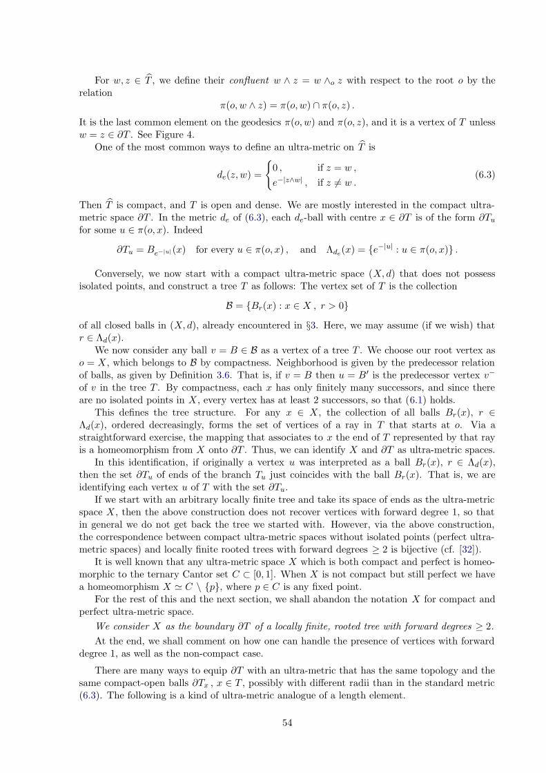
For w, z ∈ T , we define their confluent w ∧ z = w ∧o z with respect to the root o by therelation

π(o, w ∧ z) = π(o, w) ∩ π(o, z) .

It is the last common element on the geodesics π(o, w) and π(o, z), and it is a vertex of T unlessw = z ∈ ∂T . See Figure 4.

One of the most common ways to define an ultra-metric on T is

de(z, w) =

{0 , if z = w ,

e−|z∧w| , if z 6= w .(6.3)

Then T is compact, and T is open and dense. We are mostly interested in the compact ultra-metric space ∂T . In the metric de of (6.3), each de-ball with centre x ∈ ∂T is of the form ∂Tu

for some u ∈ π(o, x). Indeed

∂Tu = Be−|u|(x) for every u ∈ π(o, x) , and Λde(x) = {e−|u| : u ∈ π(o, x)} .

Conversely, we now start with a compact ultra-metric space (X, d) that does not possessisolated points, and construct a tree T as follows: The vertex set of T is the collection

B = {Br(x) : x ∈ X , r > 0}

of all closed balls in (X, d), already encountered in §3. Here, we may assume (if we wish) thatr ∈ Λd(x).

We now consider any ball v = B ∈ B as a vertex of a tree T . We choose our root vertex aso = X, which belongs to B by compactness. Neighborhood is given by the predecessor relationof balls, as given by Definition 3.6. That is, if v = B then u = B′ is the predecessor vertex v−

of v in the tree T . By compactness, each x has only finitely many successors, and since thereare no isolated points in X, every vertex has at least 2 successors, so that (6.1) holds.

This defines the tree structure. For any x ∈ X, the collection of all balls Br(x), r ∈Λd(x), ordered decreasingly, forms the set of vertices of a ray in T that starts at o. Via astraightforward exercise, the mapping that associates to x the end of T represented by that rayis a homeomorphism from X onto ∂T . Thus, we can identify X and ∂T as ultra-metric spaces.

In this identification, if originally a vertex u was interpreted as a ball Br(x), r ∈ Λd(x),then the set ∂Tu of ends of the branch Tu just coincides with the ball Br(x). That is, we areidentifying each vertex u of T with the set ∂Tu.

If we start with an arbitrary locally finite tree and take its space of ends as the ultra-metricspace X, then the above construction does not recover vertices with forward degree 1, so thatin general we do not get back the tree we started with. However, via the above construction,the correspondence between compact ultra-metric spaces without isolated points (perfect ultra-metric spaces) and locally finite rooted trees with forward degrees ≥ 2 is bijective (cf. [32]).

It is well known that any ultra-metric space X which is both compact and perfect is homeo-morphic to the ternary Cantor set C ⊂ [0, 1]. When X is not compact but still perfect we havea homeomorphism X ' C \ {p}, where p ∈ C is any fixed point.

For the rest of this and the next section, we shall abandon the notation X for compact andperfect ultra-metric space.

We consider X as the boundary ∂T of a locally finite, rooted tree with forward degrees ≥ 2.

At the end, we shall comment on how one can handle the presence of vertices with forwarddegree 1, as well as the non-compact case.

There are many ways to equip ∂T with an ultra-metric that has the same topology and thesame compact-open balls ∂Tx , x ∈ T , possibly with different radii than in the standard metric(6.3). The following is a kind of ultra-metric analogue of a length element.

54

Definition 6.1 Let T be a locally finite, rooted tree with deg+(x) ≥ 2 for all x. An ultra-metricelement is a function φ : T → (0 ,∞) with

(i) φ(v−) > φ(v) for every v ∈ T \ {o} ,

(ii) lim φ(vn) = 0 along every geodesic ray π = [v0 , v1 , v2 , . . . ] .

It induces the ultra-metric dφ on ∂T given by

dφ(x, y) =

{0 , if x = y ,

φ(x ∧ y) , if x 6= y .

The balls in this ultra-metric are again the sets

∂Tu = Bφ(u)(x) , x ∈ ∂Tu .

Note that condition (ii) in the definition is needed for having that each end of T is non-isolatedin the metric dφ . The metric de of (6.3) is of course induced by φ(x) = e−|x|.

Lemma 6.2 For a tree as in Definition 6.1, every ultra-metric on ∂T whose closed balls arethe sets ∂Tu , u ∈ T , is induced by an ultra-metric element on T .

Proof. Given an ultra-metric d as stated, we set φ(v) = diam(∂Tv), the diameter with respectto the metric d. Since deg+(v−) ≥ 2 for any v ∈ T \ {o}, the ball ∂Tv− is the disjoint unionof at least two balls ∂Tu with u− = v−. Therefore we must have diam(∂Tv) < diam(∂Tv−),and property (i) holds. Since no end is isolated, φ satisfies (ii). It is now straightforward thatdφ = d.

In view of the correspondence between the ultra-metric and the ultra-metric element, in thesequel we shall replace in the notation the subscript d referring to the metric d = dφ by thesubscript φ referring to the ultra-metric element. We note that

diamφ(∂T ) = φ(o) , Λφ(x) = {φ(u) : u ∈ π(o, x)} and Λφ = {φ(v) : v ∈ T}. (6.4)

We also note that, for any x ∈ ∂T and v ∈ π(o, x), the balls of the metric dφ satisfy the identity

Br(x) = Bφr (x) =

{∂Tv for φ(v) ≤ r < φ(v−) , if v 6= o

∂T for r ≥ φ(o) , if v = o .(6.5)

6.2 Isotropic jump processes on the boundary of a tree

In view of the explanations given above, we can consider the isotropic jump processes of (1.3)–(1.8) on the space X = ∂T . Since this space is compact, we may assume that the referencemeasure μ is a probability measure on ∂T . Given a measure μ on ∂T , a distance distributionfunction σ with properties (1.5), and an ultra-metric element φ on T , we obtain the (dφ, μ, σ)-process on ∂T , that will be referred to as the (φ, μ, σ)-process on ∂T . We can write the semigroupand its transition probabilities in detail as follows. For x ∈ ∂T and π(0, x) = [o = v0 , v1 , v2 , . . . ],using (6.5),

P tf(x) =∞∑

n=0

ctn Qφ(vn)f(x) ,

where ct0 = 1 − σt (φ(v0)) and ct

n = σt (φ(vn−1)) − σt (φ(vn)) for n ≥ 1 .

Thus, for arbitrary u ∈ T and x ∈ ∂T as above

P[Xt ∈ ∂Tu | X0 = x] =∞∑

n=0

ctn

μ(∂Tvn ∩ ∂Tu)μ(∂Tvn)

. (6.6)

The standard (d, μ)-process in the sense of Definition 2.9 in the case of metric d = dφ willbe referred to as the standard (φ, μ)-process.

55

6.3 Nearest neighbour random walks on a tree

On trees there is a class of well-studied stochastic processes, namely random walks. Our aim is toanalyze how random walks on a tree are related with isotropic jump processes on the boundaryof the tree. A good part of the material outlined next is taken from the book of Woess [63]. Anolder, recommended reference is the seminal paper of Cartier [12].

A nearest neighbour random walk on the locally finite, infinite tree T is induced by itsstochastic transition matrix P = (p(u, v))u,v∈T with the property that p(u, v) > 0 if and only ifu ∼ v. The resulting discrete-time Markov chain (random walk) is written (Zn)n≥0 . Its n-steptransition probabilities

p(n)(u, v) = Pu[Zn = v], u, v ∈ T,

are the elements of the nth power of the matrix P . The notation Pu refers to the probabilitymeasure on the space of trajectories starting at u. We assume that the random walk is transient,i.e., with probability 1 it visits any finite set only finitely often. Thus, 0 < G(u, v) < ∞ for allu, v ∈ T , where

G(u, v) =∞∑

n=0

p(n)(u, v)

is the Green kernel of the random walk. In addition, we shall also make crucial use of thequantities

F (u, v) = Pu[Zn = v for some n ≥ 0] and U(v, v) = Pv[Zn = v for some n ≥ 1] .

We shall need several identities relating them and start with a few of them, valid for all u, v ∈ T .

G(u, v) = F (u, v)G(v, v) (6.7)

G(v, v) =1

1 − U(v, v)(6.8)

U(v, v) =∑

u

p(v, u)F (u, v) (6.9)

F (u, v) = F (u,w)F (w, v) whenever w ∈ π(u, v) (6.10)

The first three identities hold for arbitrary denumerable Markov chains, while (6.10) is truespecifically for trees. The identities show that the quantities G,U, F are completely determinedjust by the values of F (u, v) for u ∼ v. More identities from [63, Chapter 9] will be cited andused later on.

By transience, the random walk Zn must converge to a random end (see e.g. [12] or [63,Theorem 9.18]).

Lemma 6.3 There is a ∂T -valued random variable Z∞ such that for every starting point u ∈ T ,

Pu[Zn → Z∞ in the topology of T ] = 1.

In brief, the argument is as follows: by transience, random walk trajectories must accumulateat ∂T almost surely. If such a trajectory had two distinct accumulation points, say x and y,then by the nearest neighbour property, the trajectory would visit the vertex x ∧u y infinitelyoften, which can occur only with probability 0.

For any u ∈ T consider the limit distribution νu that is a Borel measure on ∂T defined forany Borel set B ⊂ ∂T by

νu(B) = Pu[Z∞ ∈ B] .

56

The sets ∂Tu , u ∈ T (plus the empty set), form a semi-algebra that generates the Borel σ-algebraof ∂T . Thus, each measure νu is determined by the values on those sets. There is an explicitformula (cf. [12] or [63, Proposition 9.23]) that holds for v 6= o:

νu(∂Tv) =

F (u, v)1 − F (v, v−)

1 − F (v−, v)F (v, v−), if u ∈ {v} ∪ (T \ Tv) ,

1 − F (u, v)F (v, v−) − F (v−, v)F (v, v−)

1 − F (v−, ν)F (v, v−), if u ∈ Tv .

(6.11)

A harmonic function is a function h : T → R with Ph = h, where

Ph(u) =∑

v

p(u, v)h(v) .

For any Borel set B ⊂ ∂T , the function u 7→ νu(B) is a bounded harmonic function. It ispossible to prove that all νu are comparable in the following sense: p(k)(u, v) νu ≤ νv , where kis the length of π(u, v). Thus, for any function ϕ ∈ L1(∂T, νo), the function hϕ defined by

hϕ(u) =∫

∂Tϕdνu

is finite and harmonic on T . It is often called the Poisson transform of ϕ.Next we define a measure m on T as follows: m(o) = 1, and for v ∈ T \ {o} with π(o, v) =

[o = v0 , v1 , . . . , vk = v],

m(v) =p(v0, v1)p(v1, v2) ∙ ∙ ∙ p(vk−1, vk)p(v1, v0)p(v2, v1) ∙ ∙ ∙ p(vk, vk−1)

. (6.12)

Then, for all u, v ∈ T ,

m(u)p(u, v) = m(v)p(v, u) , and consequently m(u)G(u, v) = m(v)G(v, u) . (6.13)

Hence, the random walk is reversible. This will allow us to use the electrical network inter-pretation of (T,P , m): see e.g. Yamasaki [65], Soardi [54], or – with notation as used here –[63, Chapter 4]. Each edge e = [v−, v] ∈ E(T ) is thought of as an electric conductor withconductance

a(v−, v) = m(v)p(v, v−).

The Dirichlet form ET = ET,P for functions f, g : T → R is defined by

ET (f, g) =∑

[v−,v]∈E(T )

(f(v) − f(v−)

) (g(v) − g(v−)

)a(v−, v) . (6.14)

The domain of this Dirichlet form is the following space:

D(T ) = D(T,P) = {f : T → R | ET (f, f) < ∞}. (6.15)

6.4 Harmonic functions of finite energy and their boundary values

We are interested in the subspace

HD(T ) = HD(T,P) = {h ∈ D(T,P) : Ph = h}

of harmonic functions with finite energy. The terminology comes from the interpretation of sucha function as the potential of an electric flow (current), and then ET (h, h) is the energy of thatflow.

Every function in HD(T,P) is the Poisson transform of some function ϕ ∈ L2(∂T, νo). Thisis valid not only for trees, but for general finite range reversible Markov chains, and follows fromthe following facts.

57

(1) Every function in HD is the difference of two non-negative functions in HD.

(2) Every non-negative function in HD can be approximated by a monotone increasing se-quence of non-negative bounded functions in HD.

(3) Every bounded harmonic function is the Poisson transform of a bounded function on theboundary.

The boundary ∂T is the (active part of) the Martin boundary, with νu being the limitdistribution on ∂T of the Markov chain, starting at u. The facts (1) and (2) are contained in[65] and [54], while (3) is part of general Martin boundary theory, see e.g. [63, Theorem 7.61].

Thus, we introduce a form EHD on ∂T by setting

D(∂T,P) = {ϕ ∈ L1(∂T, νo) : ET (hϕ, hϕ) < ∞} ,

EHD(ϕ,ψ) = ET (hϕ, hψ) for ϕ,ψ ∈ D(∂T,P).(6.16)

6.5 Jump processes on the boundary of a tree

Kigami [36] elaborates an expression for the form EHD(ϕ,ψ) of (6.16) by considerable effort,shows its regularity properties and then studies the jump process on ∂T induced by this Dirichletform. We call this the boundary process associated with the random walk on T .

Let us show that there is a rather simple expression for EHD . Define the Naım kernel on∂T × ∂T by

Θo(x, y) =

m(o)G(o, o)F (o, x ∧ y)F (x ∧ y, o)

, if x 6= y ,

+∞ , if x = y .(6.17)

In our case m(o) = 1, but we do not use this to ensure the applicability of (6.17) in more generalcases (think of a different choice of the base point, or a different normalization of the measurem).

Theorem 6.4 For any transient nearest neighbour random walk on the tree T with root o, andall functions ϕ, ψ in D(∂T,P),

EHD(ϕ,ψ) =12

∫

∂T

∫

∂T(ϕ(x) − ϕ(y)) (ψ(x) − ψ(y))Θo(x, y) dνo(x) dνo(y) .

A proof of Theorem 6.4 is given in [20] in a setting of potential theory on Green spaces,which are locally Euclidean. The definition of the Naım kernel in [44] refers to the same type ofsetting. However, the trees, even when seen as metric graphs, are not locally Euclidean. In thissense, so far the definition of the Naım kernel and a proof of Theorem 6.4 in a suitable for ussetting have not been well accessible in the literature. In a forthcoming paper, Georgakopoulosand Kaimanovich will provide those “missing links” in full generality.

We give here a direct and simple proof of Theorem 6.4 for the specific case of trees. We startwith the following observation.

Lemma 6.5 The measure Θo(x, y) dνo(x) dνo(y) on ∂T ×∂T is invariant with respect to chang-ing the base point (root) o.

Proof. We want to replace the base point o with some other u ∈ T . We may assume thatu ∼ o. Indeed, then we may step by step replace the current base point by one of its neighboursto obtain the result for arbitrary u.

58

Recall that the confluent that appears in the definition (6.17)) of Θo depends on the root o,while for Θx it becomes the one with respect to x as the new root. It is a well-known fact that

dνu

dνo(x) = K(u, x) :=

G(u, u ∧o x)G(o, u ∧o x)

,

where K is called the Martin kernel. Thus, we have to show that for all x, y ∈ ∂T (x 6= y)

m(o)G(o, o)F (o, x ∧o y)F (x ∧o y, o)

=m(u)K(u, x)K(u, y)

G(u, u)F (u, x ∧u y)F (x ∧u y, u).

Consider four cases.Case 1. x, y ∈ ∂Tu. Then x ∧o y = x ∧u y =: v ∈ Tu, and u ∧o x = u ∧o y = u. Thus, using

(6.7), (6.10) and the fact that by (6.13)

m(u)/G(o, u) = m(o)/G(u, o),

we obtain

m(u)K(u, x)K(u, y)G(u, u)F (u, x ∧u y)F (x ∧u y, u)

=m(u)

G(u, u)F (u, v)F (v, u)

(G(u, u)G(o, u)

)2

=m(o)G(u, u)

F (u, v)F (v, u)G(o, u)G(u, o)

=m(o)

F (u, v)F (v, u)F (o, u)F (u, o)G(o, o)

=m(o)

F (o, v)F (v, o)G(o, o),

as required.

Case 2. x, y ∈ ∂T \ ∂Tu . Then

x ∧o y = x ∧u y =: w ∈ T \ Tu, and u ∧o x = u ∧o y = o.

Case 3. x ∈ ∂Tu , y ∈ ∂T \ ∂Tu . Then

x ∧o y = o, x ∧u y = u, u ∧o x = u and u ∧o y = o.

Case 4. x ∈ ∂T \ ∂Tu , y ∈ ∂Tu . This is similar to Case 3, exchanging the roles of x and y.

In all cases 2–4, the proof is done similarly to Case 1.For the proof of Theorem 6.4, we need a few more facts related with the network setting;

compare e.g. with [63, §4.D].The space D(T ) of (6.15) is a Hilbert space when equipped with the inner product

(f, g) = ET (f, g) + f(o)g(o) .

The subspace D0(T ) is defined as the closure of the space of finitely supported functions inD(T ). It is a proper subspace if and only if the random walk is transient, and then the functionGv(u) = G(u, v) is in D0(T ) for any v ∈ T [65], [54]. We need the formula

ET (f,Gv) = m(v)f(v) for every f ∈ D0(T ) . (6.18)

59

Given a branch Tw of T (for w ∈ T \ {o}), we can consider it as a subnetwork equipped withthe same conductances a(u, v) for [u, v] ∈ E(Tw). The associated measure on Tw is

mTw(u) =∑

v∈Tz :v∼u

a(u, v) =

{m(u) if u ∈ Tw \ {w} ,

m(w) − a(w,w−) if u = w .

The resulting random walk on Tw has transition probabilities

pTw(u, v) =a(v, w)mTw(u)

=

p(u, v) if u ∈ Tw \ {w} , v ∼ u ,

p(w, v)1 − p(w,w−)

if u = w , v ∼ u .

We have FTw(u, u−) = F (u, u−) and thus also FTw(u,w) = F (u,w) for every u ∈ Tw \ {w},because before its first visit to w, the random walk on Tw obeys the same transition probabilitiesas the original random walk on T . It is then easy to see [63, p. 241] that the random walk onTw is transient if and only if for the original random walk, F (w,w−) < 1, which in turn holdsif and only if νo(∂Tw) > 0. (In other parts of this and the preceding two sections, this is alwaysassumed, but for the proof of Theorem 6.4, we just assume the random walk on the whole of Tto be transient.) Conversely, if F (w,w−) = 1 then F (u,w) = 1 for all u ∈ Tw .

Below, we shall need the following formula for the limit distributions.

Lemma 6.6 For u ∈ T \ {o},

νu(∂Tu) = 1 − p(u, u−)(G(u, u) − G(u−, u)

).

Proof. By (7.7),

G(u, u)p(u, u−) =F (u, u−)

1 − F (u, u−)F (u−, u)

Thus,

p(u, u−)(G(u, u) − G(u−, u)

)=(1 − F (u−, u)

)G(u, u)p(u, u−) = 1 − νu(∂Tu)

after a short computation using (6.11)

Proof of Theorem 6.4. We first prove the Doob-Naım formula (shortly, D-N-formula) forthe case when ϕ = 1∂Tv and ψ = 1∂Tw for two proper branches Tv and Tw of T . They are eitherdisjoint, or one of them contains the other.

Case 1. Tw ⊂ Tv . (The case Tv ⊂ Tw is analogous by symmetry.)This means that w ∈ Tv . For x, y ∈ ∂T we have

(ϕ(x) − ϕ(y)) (ψ(x) − ψ(y)) = 1

if x ∈ ∂Tw and y ∈ ∂T \ ∂Tv or conversely, and

(ϕ(x) − ϕ(y)) (ψ(x) − ψ(y)) = 0

otherwise. By Lemma 6.5, we may choose v as the base point. Thus, the right hand side of theidentity is

∫

∂T\∂Tv

∫

∂Tw

Θv(x, y) dνv(x) dνv(y) =m(v)

G(v, v)νv(∂T \ ∂Tv)νv(∂Tw) ,

since x ∧v y = v and F (v, v) = 1.

60

Let us now turn to the left hand side of the D-N-formula. The Poisson transforms of ϕ andψ are

hϕ(u) = νu(∂Tv) and hψ(u) = νu(∂Tw).

By (6.11),

hϕ(u) = F (u, v)νv(∂Tv) , u ∈ {v} ∪ (T \ Tv)

1 − hϕ(u) = F (u, v)νv(∂T \ ∂Tv) , u ∈ Tv .

We set Fv(u) = F (u, v) and write

hϕ(u) − hϕ(u−) =(1 − hϕ(u−)

)− (1 − hϕ(u))

whenever this is convenient, and analogously for hψ . Then we get

ET (hϕ , hψ)

=∑

[u,u−]∈E(T )\E(Tv)

a(u, u−)(F (u, v) − F (u−, v)

)νv(∂Tv)

(F (u, v) − F (u−, v)

)νv(∂Tw)

−∑

[u,u−]∈E(Tv)\E(Tw)

a(u, u−)(F (u, v) − F (u−, v)

)νv(∂T \ ∂Tv)

(F (u, v) − F (u−, v)

)νv(∂Tw)

+∑

[u,u−]∈E(Tw)

a(u, u−)(F (u, v) − F (u−, v)

)νv(∂T \ ∂Tv)

(F (u, v) − F (u−, v)

)νv(∂T \ ∂Tw)

= ET (Fv , Fw)νv(∂Tv)νv(∂Tw) − ETv(Fv , Fw)νv(∂Tw) + ETw(Fv , Fw)νv(∂T \ ∂Tv) ,

where of course ETv is the Dirichlet form of the random walk on the branch Tv , as discussedabove, and analogously for ETw . Now Fv = Gv/G(v, v) by (6.7), whence (6.18) yields

ET (Fv, Fw) =ET (Gv, Fw)

G(v, v)=

m(v)F (v, w)G(v, v)

. (6.19)

Recall that for the random walk on Tv , we have FTv(u, v) = F (u, v) for every u ∈ Tv . Also,

mTv(v) = m(v) − a(v, v−) = m(v)(1 − p(v, v−)

).

We apply (6.19) to that random walk and obtain

ETv(Fv, Fw) =m(v) (1 − p(v, v−)) F (v, w)

GTv(v, v).

Applying (6.8), (6.9) and

pTv(v, u) =p(v, u)

1 − p(v, v−)

for u ∈ Tv , we obtain

1 − p(v, v−)GTv(v, v)

= 1 − p(v, v−) −(1 − p(v, v−)

)UTv(v, v)

= 1 − p(v, v−) −∑

u:u−=v

p(v, u)F (u, v)

= 1 − p(v, v−) −(U(v, v) − p(v, v−)F (v−, v)

)

=1

G(v, v)− p(v, v−)

(1 − F (v−, v)

)=

νv(∂Tv)G(v, v)

,

61

where in the last step we have used Lemma 6.6. It follows that

ETv(Fv, Fw) =m(v)F (v, w)

G(v, v)νv(∂Tv).

In the same way, exchanging roles between Tw and Tv and using reversibility (6.13),

ETw(Fv, Fw) =m(w)F (w, v)

G(w,w)νw(∂Tw) =

m(v)F (v, w)G(v, v)

νw(∂Tw) =m(v)

G(v, v)νv(∂Tw)

Putting things together, we get that

ET (hϕ , hψ) = ETw(Fv , Fw)νv(∂T \ ∂Tv) =m(v)

G(v, v)νv(∂Tw)νv(∂T \ ∂Tv),

as proposed.

Case 2. Tw ∩ Tv = ∅ .In view of Lemma 6.5, both sides of the D-N-formula are independent of the root o. Thus

we may declare our root to be one of the neighbours of v that is not on π(v, w). Also, let v bethe neighbour of v on π(w, v). Then, with our chosen new root, the complement of the “old” Tv

is Tv, which contains Tw (The latter remains the same with respect to the new root).Thus, we can apply the result of case 1 to Tv and Tw. This means that we have to replace

the functions ϕ and hϕ with 1−ϕ and 1−hϕ, respectively, which just means that we change thesign on both sides of the identity. We are re-conducted to Case 1 without further computations.

We deduce from what we have done so far, and from linearity of the Poisson transform as wellof bilinearity of the forms on both sides of the D-N-formula , that it holds for linear combinationsof indicator functions of sets ∂Tv . Those indicator functions are dense in the space C(∂T ) withrespect to the max-norm. Thus, the D-N-formula holds for all continuous functions on ∂T . Theextension to all of D(∂T,P) is by standard approximation.

7 The duality of random walks on trees and isotropic processeson their boundaries

When looking at our isotropic processes and at the boundary process of Kigami [36], it is naturalto ask the following two questions.

Question I. Given a transient random walk on T associated with the Dirichlet form ET of(6.14), does the boundary process on ∂T induced by the form EHD of (6.16) coincide with anisotropic process (1.8) on ∂T with transition probabilities (6.6), induced by the measure μ = νo

on ∂T , some ultra-metric element φ on T and a suitable distance distribution function σ on[0 , ∞) ?

Question II. Conversely, given data μ, φ and σ, is there a random walk on T with limitdistribution νo = μ such that the isotropic process induced by μ, φ and σ is the boundaryprocess with Dirichlet form EHD?

Before answering both questions, we need to specify the assumptions more precisely. Whenstarting with (φ, μ, σ), we always assume as before that μ is supported by the whole of ∂T .

Thus, on the side of the random walk, we also want that supp(νo) = ∂T . This is equivalentwith the requirement that νo(∂Tv) > 0 for every v ∈ T . By (6.11) this is in turn equivalent with

F (v, v−) < 1 for every v ∈ T \ {o}. (7.1)

62

Indeed, we shall see that we need a bit more, namely that

limv→∞

G(v, o) = 0 , (7.2)

that is, for every ε > 0 there is a finite set A ⊂ T such that G(v, o) < ε for all v ∈ T \ A. Thiscondition is necessary and sufficient for solvability of the Dirichlet problem: for any ϕ ∈ C(∂X),its Poisson transform hϕ provides the unique continuous extension of ϕ to T which is harmonicin T . See e.g. [63, Corollary 9.44].

We shall restrict attention to random walks with properties (7.1) and (7.2) on a rooted treewith forward degrees ≥ 2.

7.1 Answer to Question I

We start with a random walk that fulfills the above requirements. We know from §1 that each(μ, φ, σ)-process arises as the standard process of Definition 2.9 with respect to the intrinsicmetric (cf. Theorem 2.10): given φ and σ, the intrinsic metric is induced by the ultra-metricelement

φ∗(u) = −1/

log σ (φ(u)) . (7.3)

Thus, we can eliminate σ from our considerations by just looking for an ultra-metric element φsuch that the boundary process is the standard process on ∂T associated with (φ, ν0).

Since the processes are determined by the Dirichlet forms, we infer from Theorems 3.12 and6.4 that we are looking for φ such that J(x, y) = Θo(x, y) for all x, y ∈ ∂T with x 6= y, whereJ(x, y) is given by (3.11). Rewriting J(x, y) in terms of φ, νo and the tree structure, this becomes

1φ(o)

+∫ 1/φ(x∧y)

1/φ(o)

dt

νo

(Bφ

1/t(x)) =

m(o)G(o, o)F (o, x ∧ y)F (x ∧ y, o)

. (7.4)

In our case, m(o) = 1, but we keep track of what happens when one changes the root or thenormalisation of m. First of all, since deg+(o) ≥ 2, there are x, y ∈ ∂T such that x ∧ y = o. Weinsert these two boundary points in (7.4). Since F (o, o) = 1, we see that we must have

φ(o) = G(o, o)/m(o) .

Now take v ∈ T \ {o}. Since forward degrees are ≥ 2, there are x, y, y′ ∈ ∂T such that x∧ y = vand x ∧ y′ = v−. We write (7.4) first for (x, y′) and then for (x, y) and then take the difference,leading to the equation

∫ 1/φ(v)

1/φ(v−)

dt

νo

(Bφ

1/t(x)) =

m(o)G(o, o)F (o, v)F (v, o)

−m(o)

G(o, o)F (o, v−)F (v−, o). (7.5)

By (6.5), within the range of the last integral we must have Bφ1/t(v) = ∂Tv , whence that integral

reduces to (1

φ(v)−

1φ(v−)

)1

νo(∂Tv).

We multiply equation (7.5) by νo(∂Tv) and simplify the resulting right hand side(

m(o)G(o, o)F (o, v)F (v, o)

−m(o)

G(o, o)F (o, v−)F (v−, o)

)

νo(∂Tv)

by use of the identities (6.7) – (6.10)) and the first of the two formulas of (6.11) (for νo). Weobtain that the ultra-metric element that we are looking for should satisfy

1φ(v)

−1

φ(v−)=

m(o)G(v, o)

−m(o)

G(v−, o)for every v ∈ T \ {o} . (7.6)

63

This determines 1/φ(v) recursively, and with m(o) = 1, we obtain

φ(v) = G(v, o) .

Since by (6.7) and (6.10)G(v, o) = F (v, v−)G(v−o),

the assumptions (7.1) and (7.2) yield that φ is an ultra-metric element. Reversing the lastcomputations, we see that with this choice of φ, we have indeed that J(x, y) = Θo(x, y) for allx, y ∈ ∂T with x 6= y. Hence, we have proved the following result.

Theorem 7.1 Let T be a locally finite, rooted tree with forward degrees ≥ 2. Consider a tran-sient nearest neighbour random walk on T that satisfies (6.7) and (6.10). Then the boundaryprocess on ∂T induced by the Dirichlet form (6.16) coincides with the standard process associatedwith ultra-metric element φ = G(∙, o) and the limit distribution νo of the random walk.

Let L be the Laplacian associated with the boundary process of Theorem 7.1. L acts onlocally constant functions f by

Lf(x) =∫

∂T(f(x) − f(y))Θo(x, y) dνo(y).

In view of the identification of balls in ∂T with vertices of T, the eigenfunctions of (3.6) nowbecome

fv =1∂Tv

νo(∂Tv)−

1∂Tv−

νo(∂Tv−), v ∈ T\{o}.

In addition, we set fo = 1 and note that it is an eigenfunction of L with eigenvalue 0. ApplyingTheorem 3.8 we obtain the following.

Corollary 7.2 For v ∈ T \ {o}, we have Lfv = G(v−, o)−1fv and the set of eigenfunctions{fv}v∈T is complete. In particular, we have

specL = {G(v, o)−1 : v ∈ T} ∪ {0}.

Remark 7.3 For any two vertices v and w in T \ {o} such that v− = w− = u the functionsfv and fw are eigenfunctions of L corresponding to the eigenvalue λ = 1/G(u, o). Hence theeigenspace H(u) corresponding to the vertex u is spanned by functions {fv : v− = u}. Since therank of the system {fv : v− = u} is deg+(u)− 1, where deg+(u) ≥ 2 is the forward degree of thevertex u, we obtain

dimH(u) = deg+(u) − 1

(cf. (3.9)).

Remark 7.4 Given the random walk on T and the associated boundary process on ∂T , wemight want to realize the latter as the (νo, φ, σ)-process for an ultra-metric element φ differentfrom G(∙, o). This means that we have to look for a suitable distance distribution σ on [0 , ∞),different from the inverse exponential distribution (2.16). In view of (7.3), we are looking for σsuch that for our given generic φ,

σ (φ(v)) = e−1/G(v,o).

For this it is necessary that φ(u) = φ(v) whenever G(u, o) = G(v, o): we need φ to be constanton equipotential sets. In that case, the distribution function σ(r) is determined by the aboveequation for r in the value set Λφ of the ultra-metric dφ . Then that function can be extendedto [0, +∞).

64

7.2 Answer to Question II

Answering Question II means that we start with φ and μ and then look for a random walkwith limit distribution νo = μ such that the standard (φ, μ)-process is the boundary processassociated with the random walk. We know from Theorem 7.1 that in this case, we should haveφ(v) = G(v, o), whence in particular, φ(o) > 1. Thus we cannot expect that every φ is suitable.The most natural choice is to replace φ by C ∙ φ for some constant C > 0. For the standardprocesses associated with φ and C ∙ φ, respectively, this just gives rise of a linear time change:if the old process is {Xt}t>0, then the new one is {Xt/C}t>0 .

Theorem 7.5 Let T be a locally finite, rooted tree with forward degrees ≥ 2. Consider an ultra-metric element φ on T and a fully supported probability measure μ on ∂T . Then there are aunique constant C > 0 and a unique transient nearest neighbour random walk on T that satisfies(6.7) and (6.10) with the following properties:

1. μ = νo is the limit distribution of the random walk.

2. The associated boundary process coincides with the standard process on ∂T induced by theultra-metric element C ∙ φ and the given measure μ.

For the proof, we shall need three more formulas. The first two are taken from [63, Lemma9.35], while the third is immediate from (6.11) and (6.10)

G(u, u) p(u, v) =F (u, v)

1 − F (u, v)F (v, u)if u ∼ v , and (7.7)

G(u, u) = 1 +∑

v:v∼u

F (u, v)F (v, u)1 − F (u, v)F (v, u)

(7.8)

F (v−, v) =νo(∂Tv)/F (o, v−)

1 − F (v, v−) + F (v, v−) νo(∂Tv)/F (o, v−). (7.9)

Proof of Theorem 7.5. We proceed as follows: we start with φ and μ and replace φ by anew ultra-metric element C ∙ φ, with C to be determined, and μ being the candidate for thelimit distribution of the random walk that we are looking for.

Using the various formulas at our disposal, we first construct in the only possible way thequantities F (u, v) , u, v,∈ T , in particular when u ∼ v. In turn, they lead to the Green kernelG(u, v). So far, these will be only “would-be” quantities whose feasibility will have to be verified.Until that verification, we shall denote them F (u, v) and G(u, v). Via (7.7), they will lead todefinitions of transition probabilities p(u, v). Stochasticity of the resulting transition matrix Pwill also have to be verified.

Only then, we will use a potential theoretic argument to show that G(u, v) really is the Greenkernel associated with P , so that the question mark that is implicit in the “ ˜ ” symbol can beremoved.

First of all, in view of Theorem 7.1, we must have

C ∙ φ(v) = G(v, o) ,

whence by (6.7) and (6.10)

F (v, v−) = φ(v)/φ(v−) for v ∈ T \ {o} , (7.10)

and more generallyF (v, u) = φ(v)/φ(u) when u ≤ v .

65

We note immediately that 0 < F (v, u) < 1 when u < v, and that F (u, u) = 1.Next, we use (7.9) to construct recursively F (v−, v) and F (o, v). We start with F (o, o) = 1.

If v 6= o and F (o, v−) is already given, with

μ(∂Tv−) ≤ F (o, v−) ≤ 1

(the lower bound is required by (6.11)), then we have to set

F (v−, v) =μ(∂Tv)/F (o, v−)

1 − F (v, v−) + F (v, v−) μ(∂Tv)/F (o, v−)(7.11)

andF (o, v) = F (o, v−)F (v−, v) .

SinceF (o, v−) ≥ μ(∂Tv−) ≥ μ(∂Tv),

we see that0 < F (v−, v) ≤ 1.

We set – as imposed by (6.10) –

F (o, v) = F (o, v−)F (v−, v).

Formula (7.11) transforms into

μ(∂Tv) = F (o, v−)F (v−, v)1 − F (v, v−)

1 − F (v, v−)F (v−, v)≤ F (o, v) ≤ 1 , (7.12)

as needed for our recursive construction. At this point, we have all values of F (u, v), initiallyfor u ∼ v, and consequently for all u, v by taking products along geodesic paths.

We now can compute the constant C: (7.8), combined with (7.10) and (7.12) for u ∼ o forces

Cφ(o) = G(o, o) = 1 +∑

u:u∼o

F (o, u)F (u, o)

1 − F (o, u)F (u, o)

= 1 +∑

u:u∼o

F (u, o)

1 − F (u, o)μ(∂Tu)

= 1 +∑

u:u∼o

φ(u)/φ(o)1 − φ(u)/φ(o)

μ(∂Tu)

Therefore, we have

C =1

φ(o)+∑

u:u∼o

φ(u)/φ(o)φ(o) − φ(u)

μ(∂Tu) . (7.13)

We now construct G(u, u) via (7.8):

G(u, u) = 1 +∑

v:v∼u

F (u, v)F (v, u)

1 − F (u, v)F (v, u). (7.14)

For u = o, we know that this is compatible with our choice of C. At last, our only choice forthe Green kernel is

G(u, v) = F (u, v)G(v, v) , u, v ∈ T .

66

Now we finally arrive at the only way how to define the transition probabilities, via (7.7):

p(u, v) =1

G(u, u)

F (u, v)

1 − F (u, v)F (v, u). (7.15)

Claim 1. P is stochastic.

Proof of Claim 1. Combining (7.15) with (7.14), we deduce that we have to verify that for everyu ∈ T ,

∑

v:v∼u

F (u, v)(1 − F (v, u)

)

1 − F (u, v)F (v, u)= 1 . (7.16)

If u = o, then by (7.12) this is just∑

v:v∼o

μ(∂Tv) = 1.

If u 6= o then, again by (7.12), the left hand side of (7.16) is

∑

v:v−=u

F (u, v)(1 − F (v, u)

)

1 − F (u, v)F (v, u)+

F (u, u−)(1 − F (u−, u)

)

1 − F (u, u−)F (u−, u)

=∑

v:v−=u

μ(∂Tv)

F (o, u)+ 1 −

1 − F (u−, u)

1 − F (u, u−)F (u−, u)= 1.

This proves Claim 1.

Claim 2. For any u0 ∈ T , the function gu0(u) = G(u, u0) satisfies P gu0 = gu0 − 1u0 .

Proof of Claim 2. First, we combine (7.14) with (7.15) to get

P gu0(u0) =∑

v:v∼u0

p(u0, v)F (v, u0)G(u0, u0) =∑

v:v∼u0

F (u0, v)F (v, u0)

1 − F (u0, v)F (v, u0)= gu0(u0) − 1 ,

and Claim 2 is true at u = u0 . Second, for u 6= u0, let w be the neighbour of u on π(u, u0).Then

P gu0(u) =∑

v:v∼u,v 6=w

p(u, v)F (v, u)G(u, u0) + p(u,w)G(w, u0)

=∑

v:v∼u

F (u, v)F (v, u)

1 − F (u, v)F (v, u)︸ ︷︷ ︸

G(u,u)−1

G(u, u0)

G(u, u)− p(u,w)F (w, u)G(u, u0) + p(u,w)G(w, u0)

= G(u, u0)

(

1 −1

G(u, u)− p(u,w)F (w, u) + p(u,w)

1

F (u,w)

)

= gu0(u)

sincep(u,w)/F (u,w) − p(u,w)F (w, u) = 1/G(u, u)

by (7.15). This completes the proof of Claim 2.

Now we can conclude: the function gu0 is non-constant, positive and superharmonic. There-fore the random walk with transition matrix P given by (7.15) is transient and does posses aGreen function G(u, v). Furthermore, by the Riesz decomposition theorem, we have

gu0 = Gf + h ,

67

where h is a non-negative harmonic function and the charge f of the potential

Gf(u) =∑

v

G(u, v)f(v)

is f = gu0 − P gu0 = 1u0 . That is,

G(u, u0) = G(u, u0) + h(x) for all u ∈ T.

Now let x ∈ ∂T and v = u0 ∧ x. If u ∈ Tv then by our construction

G(u, u0) = G(u, o)G(v, u0)

φ(v)φ(u) → 0 as u → x .

Therefore G(∙, u0) vanishes at infinity, and the same must hold for h. By the Maximum Principle,h ≡ 0.

We conclude that G(u, v) = G(u, v) for all u, v ∈ T . But then, by our construction, alsoF (u, v) = F (u, v). Comparing (7.12) with (6.11), we see that μ = νo . This completes the proof.

7.3 The non-compact case

The approach of the present work is not restricted to compact spaces. In case of a non-compact,locally compact ultra-metric space without isolated points, one constructs the tree in the sameway: the vertex set corresponds to the collection of all closed balls, and neighbourhood in theresulting tree is defined as above: if a vertex v corresponds to a ball B, then the predecessorv− is the vertex corresponding to the ball B′ (see Definition 3.6), and there is the edge [v−, v].Now every vertex has a predecessor (while in the compact case, the root vertex has none), andthe tree has its root at infinity, i.e., the ultra-metric space becomes ∂∗T = ∂T \ {$}, where $is a fixed reference end of T . See Figure 5 below.

We now start with this situation: given a tree T and a reference end $ ∈ ∂T , the predecessorv− = v−$ of a vertex v with respect to $ is the neighbour of v on the geodesic π(v,$). Giventwo elements w, z ∈ T \ {$}, their confluent wf z with respect to $ is again defined as the lastcommon element on the geodesics π($,w) and π($, z), a vertex, unless v = w ∈ ∂∗T (Figure 5).Again, it is natural to assume that each vertex has at least two forward neighbours.

In this situation, for the Definition 6.1 of an ultra-metric element φ : T → (0 ,∞), we needbesides monotonicity [φ(v) < φ(v−)] that φ tends to ∞ along π(o,$), while it has to tend to 0along any geodesic going to ∂∗T . The associated ultra-metric on ∂∗T is then given in the sameway as before:

dφ(x, y) =

{0 , if x = y ,

φ(xf y) , if x 6= y .

Let us note here that also when φ does not tend to ∞ along π(x,$), this does define an ultra-metric, but then (∂∗T, dφ) will not be complete. Also, if the inequality φ(v) ≤ φ(v−) is notstrict, one gets an ultra-metric, but then the above construction of the tree of closed balls doesnot recover the original tree from (∂∗T, dφ). Finally, if φ does not tend to 0 along some geodesicπ(o, x), x ∈ ∂∗T , then x will be an isolated point in (∂∗T, dφ). (The last two observations arealso true in the compact case, for a tree with a root vertex.)

Returning to our setting, the reference measure μ of a (φ, μ, σ)-process may have infinitemass: a Radon measure supported on the whole of ∂∗T . Again, we know that it is sufficientto study the standard (φ, μ)-process. We give a brief outline of the duality of such processeswith random walks on T . This should be compared with the final part of Kigami’s second paper

68

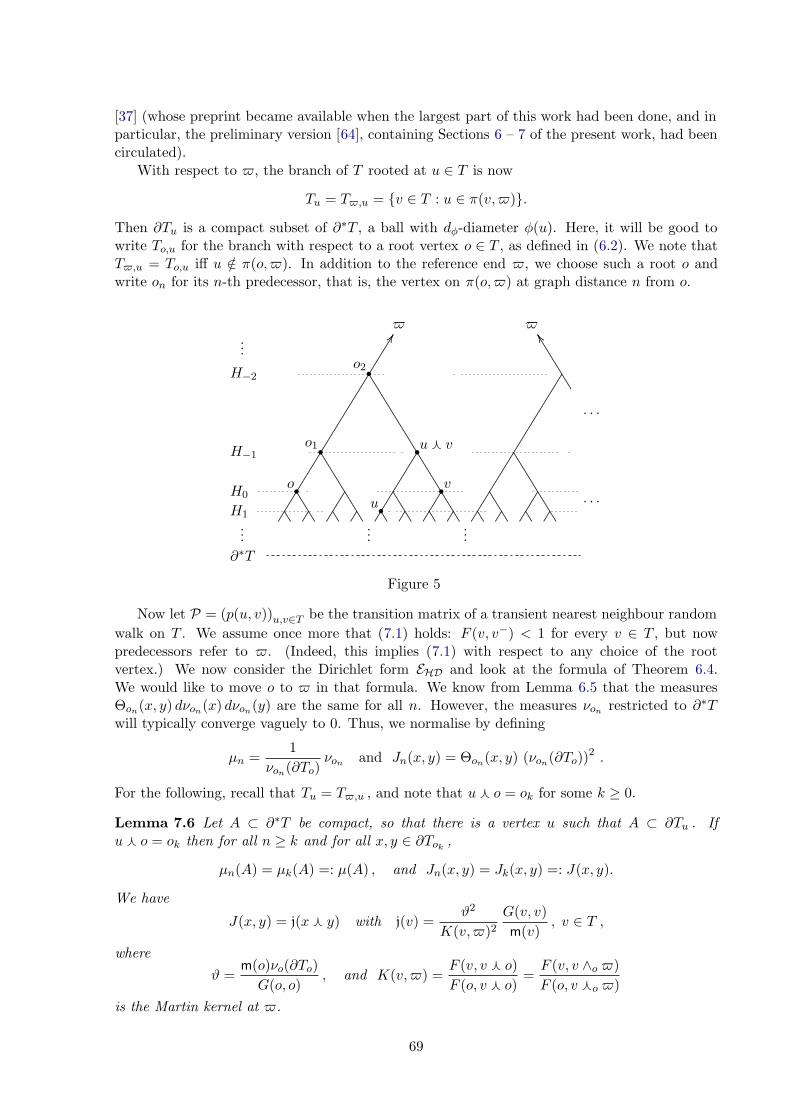
[37] (whose preprint became available when the largest part of this work had been done, and inparticular, the preliminary version [64], containing Sections 6 – 7 of the present work, had beencirculated).

With respect to $, the branch of T rooted at u ∈ T is now

Tu = T$,u = {v ∈ T : u ∈ π(v,$)}.

Then ∂Tu is a compact subset of ∂∗T , a ball with dφ-diameter φ(u). Here, it will be good towrite To,u for the branch with respect to a root vertex o ∈ T , as defined in (6.2). We note thatT$,u = To,u iff u /∈ π(o,$). In addition to the reference end $, we choose such a root o andwrite on for its n-th predecessor, that is, the vertex on π(o,$) at graph distance n from o.

.............................................................................................................................................................................................................................................................................................................................................................................................................................................................

......................................................................................................................................................................................................................................................................................................................................

.........................................................................................................................................................

.........................................................................................................................................................

..................................................................

..................................................................

..................................................................

..................................................................

......................

......................

......................

......................

......................

......................

......................

......................

........................................................................................................................................................

......................................................................................................................................................................................................................................................................................................................................

......................

......................

..................................................................

..................................................................

......................

......................

.........................................................................................................................................................

......

. . .

. . .

H−2

H−1

H0

H1

∂∗T

...

...

•o

•o1

•o2

•u

•v

•uf v

$ $

Figure 5

Now let P = (p(u, v))u,v∈T be the transition matrix of a transient nearest neighbour randomwalk on T . We assume once more that (7.1) holds: F (v, v−) < 1 for every v ∈ T , but nowpredecessors refer to $. (Indeed, this implies (7.1) with respect to any choice of the rootvertex.) We now consider the Dirichlet form EHD and look at the formula of Theorem 6.4.We would like to move o to $ in that formula. We know from Lemma 6.5 that the measuresΘon(x, y) dνon(x) dνon(y) are the same for all n. However, the measures νon restricted to ∂∗Twill typically converge vaguely to 0. Thus, we normalise by defining

μn =1

νon(∂To)νon and Jn(x, y) = Θon(x, y) (νon(∂To))

2 .

For the following, recall that Tu = T$,u , and note that uf o = ok for some k ≥ 0.

Lemma 7.6 Let A ⊂ ∂∗T be compact, so that there is a vertex u such that A ⊂ ∂Tu . Ifuf o = ok then for all n ≥ k and for all x, y ∈ ∂Tok

,

μn(A) = μk(A) =: μ(A) , and Jn(x, y) = Jk(x, y) =: J(x, y).

We have

J(x, y) = j(xf y) with j(v) =ϑ2

K(v,$)2G(v, v)m(v)

, v ∈ T ,

where

ϑ =m(o)νo(∂To)

G(o, o), and K(v,$) =

F (v, v f o)F (o, v f o)

=F (v, v ∧o $)F (o, v fo $)

is the Martin kernel at $.

69

Proof. Since ∂Tokcontains both ∂To and A, we have for n ≥ k

μn(A) =νon(A)

νon(∂To)=

F (on, ok)νok(A)

F (on, ok)νok(∂To)

= μk(A).

Analogously, Let x, y ∈ ∂Tokand xfy = v, an element of Tok

. We use the identity m(v)G(v, w) =m(w)G(w, v), which implies m(on)F (on, o) = m(on)G(on, o)/G(o, o) = m(o)G(o, on)/G(o, o),and compute for n ≥ k

Jn(x, y) =νon(∂To)2 m(on)F (on, v)G(v, on)

= νo(∂To)2 m(on)2F (on, o)2

m(on)F (on, v)G(v, on)

=νo(∂To)2m(o)2

G(o, o)2G(o, on)2

G(v, on)2G(v, v)m(v)

,

which yields the proposed formula, since G(o, on) = F (o, o f v)G(o f v, on) and G(v, on) =F (v, o f v)G(of v, on).

Now its is not hard to deduce the following.

Theorem 7.7 Let T and its reference end $ be as outlined above. Consider a nearest neighbourrandom walk on T that satisfies F (v, v−) < 1 for every v ∈ T . Let μ and J be as in Lemma 7.6.Then for all compactly supported continuous functions ϕ,ψ on ∂∗T , the Dirichlet form (6.16)can be written as

EHD(ϕ,ψ) = EJ(ϕ,ψ) + ϑ ∙ νo({$})∫

∂∗Tϕ(x)ψ(x) dμ(x) , where

EJ(ϕ,ψ) =12

∫

∂∗T

∫

∂∗T(ϕ(x) − ϕ(y)) (ψ(x) − ψ(y)) J(x, y) dμ(x) dμ(y) .

When the random walk is regular, that is, νo({$}) = 0, the form EJ = EHD induces the standard(μ, φ)-process, where the ultra-metric element φ with respect to $ is given by

φ(v) =1ϑ

K(v,$) ,

and ϑ and the Martin kernel K(v,$) are as defined in Lemma 7.6.In particular, the (μ, φ)-process is the boundary process with a time-change.

Proof. There is k such that the compact supports of ϕ and ψ are contained in ∂Tok. Let n ≥ k.

Using lemmas 6.5 and 7.6,

EHD(ϕ,ψ) =12

∫

∂T

∫

∂T(ϕ(x) − ϕ(y)) (ϕ(x) − ϕ(y)) Jn(x, y) dμn(x) dμn(y)

=12

∫

∂Ton

∫

∂Ton

(ϕ(x) − ϕ(y)) (ϕ(x) − ϕ(y)) J(x, y) dμ(x) dμ(y)

+∫

∂Ton

ϕ(x)ψ(x)∫

∂T\∂Ton

Jn(x, y) dμn(y)

︸ ︷︷ ︸=:fn(x)

dμ(x)

As n → ∞,

12

∫

∂Ton

∫

∂Ton

(ϕ(x) − ϕ(y)) (ϕ(x) − ϕ(y)) J(x, y) dμ(x) dμ(y) → EJ (ϕ,ψ) .

70

Let us look at the second term. We have

fn(x) =∫

∂T\∂Ton

Θon(x, y) νon(∂To) dνon(y).

For x ∈ ∂Ton and y ∈ ∂T \ ∂Ton , their confluent with respect to on is on itself. Therefore, using(6.17) and (6.11)

Θon(x, y) νon(∂To) =m(on)

G(on, on)F (on, o) νo(∂To) =

m(on)G(on, o)G(on, on)G(o, o)

νo(∂To)

=m(o)G(o, on)

G(on, on)G(o, o)νo(∂To) =

m(o)G(o, o)

νo(∂To) F (o, on) = ϑF (o, on) .

Now note that for y ∈ ∂T \ ∂Ton , we have F (o, on) dνon(y) = dνo(y). Therefore

fn(x) = ϑ

∫

∂T\∂Ton

F (o, on) dνon(y) = ϑ ∙ νo(∂T \ ∂Ton) → ϑ ∙ νo({$}) ,

and as n → ∞ , we can use dominated convergence to get that∫

∂Ton

ϕ(x)ψ(x)∫

∂T\∂Ton

Jn(x, y) dμn(y) dμ(x) =∫

∂∗Tϕ(x)ψ(x) fn(x) dμ(x)

→ ϑ ∙ νo({$})∫

∂∗Tϕ(x)ψ(x) dμ(x) ,

as proposed. To prove the formula for the associated ultra-metric element, we proceed as in theproof of Theorem 7.1, see (7.4) and the subsequent lines. We find that the ultra-metric elementmust satisfy

1φ(v)

−1

φ(v−)=(j(v) − j(v−)

)μ(∂Tv) .

The right hand side of this equation can be computed: we have v−f o = ok for some k ≥ 0, andcombining the arguments after (7.4) with those of the proof of Lemma 7.6,

(j(v) − j(v−)

)μ(∂Tv) =

(m(ok)

F (ok, v)G(v, ok)−

m(ok)F (ok, v−)G(v−, ok)

)

νok(∂Tv) νok

(∂To)

=

(m(ok)

G(v, ok)−

m(ok)G(v−, ok)

)

F (ok, o) νo(∂To)

=

(G(o, ok)G(v, ok)

−G(o, ok)

G(v−, ok)

)m(o)νo(∂To)

G(o, o)=

ϑ

K(v,$)−

ϑ

K(v−, $)

We infer that 1/φ(∙) − ϑ/K(∙, $) must be constant. By the regularity of the random walk,K(v,$) → ∞ as v → $. On the other hand, also φ(on) must tend to infinity. Thus, theconstant is 0, and φ has the proposed form.

Lemma 7.6 and Theorem 7.7 lead to clearer insight and simpler proofs concerning the materialon random walks in [37, §10 – §11], in particular [37, Theorem 11.3]. Namely, our limit measureμ coincides with the ν∗ of [37]. Note, that there are examples where μ(∂∗T ) = ∞, as well asexamples where μ(∂∗T ) < ∞, even though the ultra-metric space is non-compact.

Remark 7.8 In Sections 6 – 7, we have always assumed that the ultra-metric space has noisolated points, which for the tree means that deg+ ≥ 2. Theme of [7] is the opposite situation,where all points are isolated, i.e., the space is discrete. In that case the ultra-metric space isalso the boundary of a tree, which does not consist of ends, but of terminal vertices, that is,vertices with only one neighbour.

71

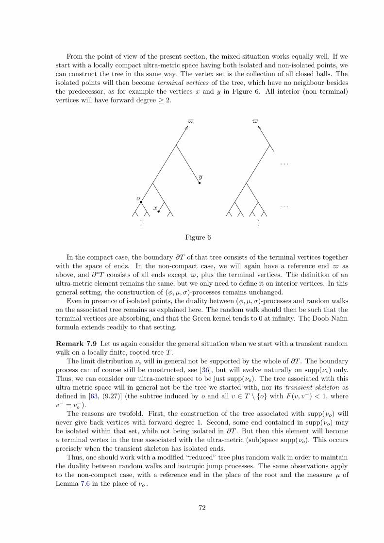
From the point of view of the present section, the mixed situation works equally well. If westart with a locally compact ultra-metric space having both isolated and non-isolated points, wecan construct the tree in the same way. The vertex set is the collection of all closed balls. Theisolated points will then become terminal vertices of the tree, which have no neighbour besidesthe predecessor, as for example the vertices x and y in Figure 6. All interior (non terminal)vertices will have forward degree ≥ 2.

.............................................................................................................................................................................................................................................................................................................................................................................................................................................................

.......................................................................................................................................................................................................................................................................................................................................

..................................................................

..................................................................

......................

......................

........................................................................................................................................................

......................................................................................................................................................................................................................................................................................................................................

......................

......................

..................................................................

..................................................................

......................

......................

.........................................................................................................................................................

......

. . .

. . .

•o

•

$ $

•x

y

Figure 6

In the compact case, the boundary ∂T of that tree consists of the terminal vertices togetherwith the space of ends. In the non-compact case, we will again have a reference end $ asabove, and ∂∗T consists of all ends except $, plus the terminal vertices. The definition of anultra-metric element remains the same, but we only need to define it on interior vertices. In thisgeneral setting, the construction of (φ, μ, σ)-processes remains unchanged.

Even in presence of isolated points, the duality between (φ, μ, σ)-processes and random walkson the associated tree remains as explained here. The random walk should then be such that theterminal vertices are absorbing, and that the Green kernel tends to 0 at infinity. The Doob-Naımformula extends readily to that setting.

Remark 7.9 Let us again consider the general situation when we start with a transient randomwalk on a locally finite, rooted tree T .

The limit distribution νo will in general not be supported by the whole of ∂T . The boundaryprocess can of course still be constructed, see [36], but will evolve naturally on supp(νo) only.Thus, we can consider our ultra-metric space to be just supp(νo). The tree associated with thisultra-metric space will in general not be the tree we started with, nor its transient skeleton asdefined in [63, (9.27)] (the subtree induced by o and all v ∈ T \ {o} with F (v, v−) < 1, wherev− = v−o ).

The reasons are twofold. First, the construction of the tree associated with supp(νo) willnever give back vertices with forward degree 1. Second, some end contained in supp(νo) maybe isolated within that set, while not being isolated in ∂T . But then this element will becomea terminal vertex in the tree associated with the ultra-metric (sub)space supp(νo). This occursprecisely when the transient skeleton has isolated ends.

Thus, one should work with a modified “reduced” tree plus random walk in order to maintainthe duality between random walks and isotropic jump processes. The same observations applyto the non-compact case, with a reference end in the place of the root and the measure μ ofLemma 7.6 in the place of νo .

72

Remark 7.10 Given a transient random walk on the rooted tree T , [36] also recovers an in-trinsic metric of the boundary process on ∂T (compact case !) in terms of what is called anultra-metric element in the present paper. This is of course φ(x) = G(x, o), denoted Dx in [36],where it is shown that for νo-almost every ξ ∈ ∂T , Dx → 0 along the geodesic ray π(o, ξ). Thishas the following potential theoretic interpretation.

A point x ∈ ∂T is called regular for the Dirichlet problem, if for every ϕ ∈ C(∂T ), its Poissontransform hϕ satisfies

limv→x

hϕ(v) = ϕ(x).

It is known from Cartwright, Soardi and Woess [14, Remark 2] that x is regular if and onlyif limu→x G(u, o) = 0 (as long as T has at least 2 ends), see also [63, Theorem 9.43]. By thelatter theorem, the set of regular points has νo-measure 1. That is, the Green kernel vanishesat νo-almost every boundary point.

Remark 7.11 In the proof of Theorem 7.5, we have reconstructed random walk transitionprobabilities from C ∙ φ(u) = G(u, o) and μ = νo .

A similar (a bit simpler) question was addressed by Vondracek [60]: how to reconstruct thetransition probabilities from all limit distributions νu , u ∈ T , on the boundary. The method of[60] as well as our method basically come from (6.11) and (7.7)-(7.8), which can be traced backto Cartier [12].

8 Random walk associated with p-adic fractional derivative

In this section we consider a two-fold specific example which unites the approaches of Section 5and Sections 6–7. We start with the compact case.

8.1 The p-adic fractional derivative on Zp

Let Zp ⊂ Qp be the group of p-adic integers. As a counterpart of the operator Dα we introducethe operator Dα of fractional derivative on Zp . We show that it is the Laplacian of an appropriateisotropic Markov semigroup. Then we construct a random walk associated with Dα in the senseof Sections 6–7.

Since Zp is a compact Abelian group, its dual Zp is a discrete Abelian group. It is knownthat the group Zp can be identified with the group

Z(p∞) = {p−nm : 0 ≤ m < pn, n = 1, 2, ...}

equipped with addition of numbers mod 1 as the group operation. As sets (but not as groups)Z(p∞) ⊂ Qp , whence the function ξ 7→ ‖ξ‖p is well-defined on the group Z(p∞).

Definition 8.1 The operator (Dα,Vc), α > 0, is defined via the Fourier transform on thecompact Abelian group Zp by

Dαf(ξ) = ‖ξ‖αp f(ξ), ξ ∈ Z(p∞) ,

where Vc is the space of locally constant functions on Zp .

Compare with the Definition 5.1 of the operator Dα.An immediate consequence is that the operator Dα is a non-negative definite self-adjoint

operator whose spectrum coincides with the range of the function

ξ 7→ ‖ξ‖αp : Z(p∞) → R+,

73

that is,specDα = {0, pα, p2α, ...}.

The eigenspace H(λ) of the operator Dα corresponding to the eigenvalue λ = pkα, k ≥ 1, isspanned by the function

fk =1

μp(pkZp)1pkZp

−1

μp(pk−1Zp)1pk−1Zp

and its shifts fk(∙ + a) with any a ∈ Zp/pkZp.Indeed, computing the Fourier transform of the function fk,

fk(ξ) = 1{‖ξ‖p≤pk} − 1{‖ξ‖p≤pk−1} = 1{‖ξ‖p=pk},

we obtainDαfk(ξ) = ‖ξ‖α

p fk(ξ) = pkαfk(ξ).

The maximal number of linearly independent functions in the set {fk(∙ + a) : a ∈ Zp/pkZp} ispk−1( p − 1), whence

dimH(λ) = pk−1(p − 1).

All the above shows that Dα coincides with the Laplacian of some isotropic Markov semigroup(Pt

α)t>0 on the ultra-metric measure space (Zp, dp, μp). In particular, using the complete de-scription of specDα we compute the intrinsic distance, call it dp,α(x, y),

dp,α(x, y) =

(‖x − y‖p

p

)α

.

It is now straightforward to compute the spectral distribution function Nα(x, τ ) ≡ Nα(τ) andthen the jump-kernel Jα(x, y) ≡ Jα(x − y) of the operator Dα. We claim that

Jα(x, y) =pα − 1

1 − p−α−1

(p−α − p−α−1

1 − p−α+

1

‖x − y‖1+αp

)

. (8.1)

Recall for comparison that according to (5.5) the jump-kernel Jα(x, y) of the operator Dα isgiven by

Jα(x, y) =pα − 1

1 − p−α−1

1

‖x − y‖1+αp

.

To prove (8.1), we compute Jα(z). Let ‖z‖p = p−l, then dp,α(0, z) = p−(l+1)α and

Jα(z) =

1/dp,α(0,z)∫

0

Nα(τ)dτ =

p(l+1)α∫

0

Nα(τ)dτ.

The function Nα(τ) is a non-decreasing, left-continuous staircase function having jumps at thepoints τk = pkα, k = 1, 2, ..., and taking values at these points Nα(τk) = pk−1, whence

Jα(z) = 1 ∙ pα + p(p2α − pα) + p2(p3α − p2α) + ... + pl(p(l+1)α − plα)

=1 − p−1

1 − p−α−1+

pα − 11 − p−α−1

pl(α+1)

=pα − 1

1 − p−α−1

(p−α − p−α−1

1 − p−α+

1

‖z‖1+αp

)

74

as desired. Next, we apply Theorem 3.12 and obtain

Dαf(x) =∫

Zp

(f(x) − f(y)) Jα(x − y) dμp(y). (8.2)

The equations (8.1)–(8.2) and (5.1) now yield the following result.

Corollary 8.2 For any function f defined on Zp ⊂ Qp we set f = f on Zp and 0, otherwise.Then

f ∈ dom(Dα) =⇒ f ∈ dom(Dα),

Dαf(x) = Dαf(x) and (Dαf, f) =(Dαf , f

)(8.3)

whenever x ∈ Zp, f ∈ dom(Dα) and (1, f) = 0.

8.2 Nearest neighbour random walk on the rooted tree Top

As an illustration of Theorem 7.5 we construct a random walk on the rooted tree associated withZp whose boundary process coincides with the isotropic process driven by the operator C ∙ Dα,where C = p−α(1 − p−α).

The Abelian group Zp can be identified with the boundary of the tree Top with root o where

every vertex v has p forward neighbours. In our identification, this is the tree of balls of theultra-metric space (Zp, dp) with root o corresponding to the whole of Zp and the ultra-metricdp(x, y) = ‖x − y‖p . See Figure 4 above, where p = 2. We fix a constant c ∈ (0, 1) and considerthe nearest neighbour random walk on To

p with

p(v, v−) = 1 − c and p(v−, v) =

{1/p if v− = oc/p otherwise

. (8.4)

Using [63, Thm. 1.38 and Prop. 9.3 ] one can compute precisely the Green function G(v, o), thehitting probability F (v, o) and other quantities associated with our random walk. In particular,choosing c = (1 + p−α)−1, we obtain

F (v, o) = p−α|v| and G(v, o) =p−α|v|

1 − p−α, (8.5)

where |v| is the graph distance from v to o. We see that the Green function vanishes at infinity,whence the random walk is Dirichlet regular.

The transition probabilities are invariant with respect to all automorphisms of the tree. Everysuch automorphism must fix o and every level of the tree. Let ν = νo be the limit distribution on∂To

p of the random walk starting at o. Then also ν is invariant under the automorphism groupof the tree (whose action extends to the boundary). In particular it is invariant under the actionof Zp. Thus, under the identification of ∂To

p with Zp, we have that ν = μp , the normalized Haarmeasure of Zp .

We now look at the boundary process induced by our random walk as a jump process on Zp .By Theorem 7.1, the boundary process arises as an isotropic jump process with the referencemeasure μp. Let L be its Laplacian. By Corollary 7.2, the set specL coincides with the range ofthe function v 7→ 1/G(v, o), v ∈ To

p , together with {0}. In view of the above formula for G(v, o)this means that

specL = {0, (1 − p−α), pα(1 − p−α), p2α(1 − p−α), . . . }.

Remember that

specDα = {0, pα, p2α, . . . } =pα

1 − p−αspecL.

75

Since both Dα and L have the same orthonormal basis of eigenfunctions, we conclude that theyare proportional, that is,

Dα =pα

1 − p−αL. (8.6)

Thus, finally we come to the following conclusion

Proposition 8.3 The boundary process {Xt}t>0 associated with the random walk defined in(8.4) with parameter c = (1 + p−α)−1 and the isotropic jump process {Xα

t }t>0 driven by theoperator Dα are related by the linear time change Xt/C = Xα

t , where C = p−α(1 − p−α).

The equation (8.6) implies that the jump kernel Jα(x, y) of operator Dα and the Doob-Naımkernel Θo(x, y) of operator L are related by

Jα(x, y) =pα

1 − p−αΘo(x, y). (8.7)

We now show how to compute the Doob-Naım kernel

Θo(x, y) =1

G(o, o)F (o, v)F (v, o), where v = x ∧ y,

directly, using the data of (8.5). We do not yet have F (o, v). We shall compute

N(v) =1

F (o, v)F (v, o).

Since it depends only on the level k of v, we consider an arbitrary geodesic ray [o = v0, v1, ...]and set up a linear recursion for N(vk). Denoting by w1 an arbitrary neighbour of o differentfrom v1 and applying [63, Prop. 9.3(b)] and (8.5), we obtain

F (o, v1) =1p

+p − 1

pF (w1, o)F (o, v1) =

1p

+(p − 1)p−α

pF (o, v1),

whence

F (o, v1) =pα

pα+1 − p + 1.

Thus, we get the initial values

N(v0) = 1 and N(v1) = pα+1 − p + 1.

Next, for k ≥ 1, we let wk+1 be a forward neighbour of vk different from vk+1. Applying onceagain [63, Prop. 9.3(b)] and (8.5), we obtain

F (vk, vk+1) =pα

p(pα + 1)+

(p − 1)pα

p(pα + 1)F (wk+1, vk)F (vk, vk+1)

+1

pα + 1F (vk−1, vk)F (vk, vk+1).

We insert the value F (wk+1, vk) = p−α and divide by

F (o, vk+1) = F (o, vk)F (vk, vk+1) = F (o, vk−1)F (vk−1, vk)F (vk, vk+1).

Then we get

1F (o, vk)

=pα

p(pα + 1)1

F (o, vk+1)+

p − 1p(pα + 1)

1F (o, vk)

+1

pα + 11

F (o, vk−1).

76

Now we multiply both sides with 1/F (vk, o) = pαk and get

N(vk) =1

p(pα + 1)N(vk+1) +

p − 1p(pα + 1)

N(vk) +pα

pα + 1N(vk−1).

This is a homogeneous second order linear recursion with constant coefficients. Its characteristicpolynomial has roots 1 and pα+1. Therefore

N(vk) = A + Bp(α+1)k.

Inserting the initial values we easily find the values of A and B. In order to get the Naım kernel,we have to multiply by 1/G(o, o) = 1 − p−α. Thus, we get

Θo(x, y) =(1 − p−α)(p − 1)

pα+1 − 1+

(1 − p−α)(pα+1 − p)pα+1 − 1

p(α+1)k =1 − p−α

pαJα(x, y) ,

as desired.

8.3 The random walk corresponding to Dα on Qp

Now we construct the random walk corresponding to the fractional derivative on the whole ofQp using Lemma 7.6 and Theorem 7.7 concerning the duality between isotropic processes andrandom walks in the non-compact case.

The tree associated with Qp is the homogenous tree T = Tp with degree p + 1. We have tochoose a reference end $. Then we can identify its lower boundary ∂∗Tp with the field of p-adicnumbers. With respect to $, every vertex v has its predecessor v− and p successors. Everysubtree Tv = T$,v is isomorphic with the rooted tree To

p considered above in the compact case ofthe p-adic integers. In particular, we choose the root vertex o such that ∂To = Zp . See Figure 5above, where p = 2.

We now define the random walk on Tp as in (8.4), but with predecessors referring to $ :

p(v, v−) = 1 − c and p(v−, v) = c/p , where c = (1 + p−α)−1. (8.8)

For the following quantities, see e.g. [62, pp. 423-424]. For all v ∈ Tp ,

F (v, v−) = p−α , F (v−, v) = p−1 , G(v, v) =1 + p−α

1 − p−α−1and νv(∂Tv) =

1 − p−α

1 − p−α−1.

This yields that the reference measure μ of the boundary process with respect to $, as given byLemma 7.6, is the standard Haar measure of Qp .

We compute ϑ = (1− p−α)/(1+ p−α). Furthermore, let us set h(v) = d(v, vf o)− d(o, vf o)(where d is the graph metric). This is the horocycle number of v. That is, the vertices withh(v) = k, k ∈ Z, are the elements in the k-th generation Hk of the tree (see Figure 5), and ∂Tv

corresponds to a ball with radius p−k in the standard ultra-metric of Qp . Then

K(v,$) = pα h(v) and m(v) = p(α−1)h(v).

Putting things together, we get

φ(v) =1 + p−α

1 − p−αp−α h(v) and j(v) =

(1 − p−α)2

(1 + p−α)(1 − p−α−1)p(α+1) h(v)

Retranslating this into p-adic notation, we conclude that the intrinsic metric and jump kernelof the boundary process with respect to $ are given by

dφ(x, y) =1 − p−α

1 + p−α‖x − y‖α

p and

J(x, y) =(1 − p−α)2

(1 + p−α)(1 − p−α−1)1

‖x − y‖α+1p

=1 − p−α

pα + 1Jα(x, y) ,

where Jα is the jump kernel associated with Dα. So at last, we get the following.

77

Proposition 8.4 The boundary process {Xt}t>0 with respect to the reference end $ associatedwith the random walk (8.8) on Tp and the isotropic jump process {Xα

t }t>0 driven by the operatorDα on Qp are related by the linear time change Xt/C∗ = Xα

t , where C∗ = (1 − p−α)/(pα + 1).

References

[1] S. Albeverio and W. Karwowski, Diffusion on p-adic numbers, Gaussian random fields(Nagoya, 1990), Ser. Probab. Statist., vol. 1, World Sci. Publ., River Edge, NJ, 1991,pp. 86–99.

[2] , A random walk on p-adics: generator and its spectrum, Stochastic Processes andtheir Applications 53 (1994), 1–22.

[3] S. Albeverio and X. Zhao, On the relation between different constructions of random walkson p-adics, Markov Process. Related Fields 6 (2000), 239–255.

[4] D. Aldous and St. N. Evans, Dirichlet forms on totally disconnected spaces and bipartiteMarkov chains, J. Theoret. Probab. 12 (1999), 839–857.

[5] A. Bendikov, B. Bobikau, and Ch. Pittet, Some spectral and geometric aspects of count-able groups, Random Walks, Boundaries and Spectra, Progress in Probability, vol. 64,Birkhauser, Basel, 2011, pp. 227–234.

[6] A. Bendikov, B. Bobikau, and Ch. Pittet, Spectral properties of a class of random walks onlocally finite groups, Groups, Geometry and Dynamical Systems 7 (2013), 791–820.

[7] A. Bendikov, A. Grigor’yan, and Ch. Pittet, On a class of Markov semigroups on discreteultra-metric spaces, Potential Anal. 37 (2012), 125–169.

[8] A. Bendikov and P. Krupski, On the spectrum of the hierarchical Laplacian,arXiv:1308.4883v2, to appear in POTA (2014).

[9] A. Bendikov and L. Saloff-Coste, Random walks on some countable groups, preprint (2011).

[10] C. Berg and G. Forst, Potential theory on locally compact abelian groups, Springer-Verlag,1975.

[11] S. Brofferio and W. Woess, On transience of card shuffling, Proc. Amer. Math. Soc. 129(2001), 1513–1519.

[12] P. Cartier, Fonctions harmoniques sur un arbre, Symposia Math. 9 (1972), 203–270.

[13] D. I. Cartwright, Random walks on direct sums of discrete groups, J. Theoret. Probab. 1(1988), 341–356.

[14] D. I. Cartwright, P. M. Soardi, and W. Woess, Martin and end compactifications of nonlocally finite graphs, Transactions Amer. Math. Soc. 338 (1993), 670–693.

[15] Z.-Q. Chen, M. Fukushima, and J. Ying, Traces of symmetric Markov processes and theircharacterizations, Ann. Probab. 34 (2006), 1052–1102.

[16] T. Coulhon, A. Grigor’yan, and Ch. Pittet, A geometric approach to on-diagonal heat kernellow bounds on groups, Ann. Inst. Fourier (Grenoble). 51 (2001), 1763–1827.

78

[17] D. A. Darling and P. Erdos, On the recurrence of a certain chain, Proc. Amer. Math. Soc.13 (1962), 447–450.

[18] C. Dellacherie, S. Martinez, and J. San Martin, Ultrametric matrices and induced Markovchains, Adv. Appl. Math. 17 (1996), 169–183.

[19] , Ultrametric and tree potential, J. Theoret. Probab. 22 (2009), 311–347.

[20] J. L. Doob, Boundary properties for functions with finite Dirichlet integrals, Ann. Inst.Fourier (Grenoble) 12 (1962), 573–621.

[21] J. Douglas, Solution of the problem of Plateau, Trans. Amer. Math. Soc. 33 (1931), 263–321.

[22] St. N. Evans, Local properties of Levy processes on a totally disconnected group, J. Theoret.Probab. 2 (1989), 209–259.

[23] , Local field Brownian motion, J. Theoret. Probab. 6 (1993), 817–850.

[24] , Local fields, Gaussian measures, and Brownian motions, Topics in probabilityand Lie groups: boundary theory, CRM Proc. Lecture Notes, vol. 28, Amer. Math. Soc.,Providence, RI, 2001, pp. 11–50.

[25] N. Fereig and S. A. Molchanov, Random walks on abelian groups with an infinite numberof generators, Vestnik Moskov. Univ. Ser. I Mat. Mekh. 5 (1978), 22–29.

[26] L. Flatto and J. Pitt, Recurrence criteria for random walks on countable abelian groups,Illinois J. Math. 18 (1974), 1–19.

[27] M. Fukushima, Y. Oshima Y., and M. Takeda, Dirichlet forms and symmetric Markovprocesses, 2nd ed., Walter de Gruyter, Berlin, 2011.

[28] M. Gromov, Asymptotic invariants of infinite groups, Geometric group theory, Vol. 2 (Sus-sex, 1991), London Math. Soc. Lecture Note Ser., vol. 182, Cambridge Univ. Press, Cam-bridge, 1993, pp. 1–295.

[29] S. Haran, Riesz potentials and explicit sums in arithmetic, Invent. Math. 101 (1990), 697–703.

[30] , Analytic potential theory over the p-adics, Ann. Inst. Fourier (Grenoble) 43 (1993),905–944.

[31] E. Hewitt and K. A. Ross, Abstract harmonic analysis, 1: Structure of topological groups,integration theory, group representations, Grundlehren der math. Wiss., vol. 115, Springer-Verlag, Berlin, 1963.

[32] B. Hughes, Trees and ultrametric spaces: a categorical equivalence, Adv. Math. 189 (2004),148–191.

[33] R. S. Ismagilov, On the spectrum of a selfadjoint operator in L2(K), where K is a localfield; an analogue of the Feynman-Kac formula, Teoret. Mat. Fiz. 89 (1991), 18–24.

[34] M. A. Kasymdzhanova, Recurrence of invariant Markov chains on a class of abelian groups,Vestnik Moskov. Univ. Ser. I Mat. Mekh. 3 (1981), 3–7.

[35] H. Kesten and F. Spitzer, Random walks on countably infinite abelian groups, Acta. Math.114 (1965), 237–265.

79

[36] J. Kigami, Dirichlet forms and associated heat kernels on the Cantor set induced by randomwalks on trees, Adv. Math. 225 (2010), 2674–2730.

[37] , Transitions on a noncompact Cantor set and random walks on its defining tree ,Annales de l’Institut Henri Poincare Prob.& Stat. 49 (2013), 1090–1129.

[38] A. N. Kochubeı, Parabolic equations over the field of p-adic numbers, Izv. Akad. Nauk SSSRSer. Mat. 55 (1991), 1312–1330.

[39] A. N. Kochubei, Pseudo-differential equations and stochastics over non-Archimedean fields ,Monographs and Textbooks in Pure and Applied Mathematics, vol. 244, Marcel DekkerInc., New York, 2001.

[40] G. F. Lawler, Recurrence and transience for a card shuffling model, Combin. Probab. Com-put. 4 (1995), 133–142.

[41] S. Martinez, D. Remenik, and J. San Martin, Level-wise approximation of a Markov processassociated to the boundary of an infinite tree, J. Theor. Probab. 20 (2007), 561–579.

[42] M. Del Muto and A. Figa-Talamanca, Diffusion on locally compact ultrametric spaces, Expo.Math. 22 (2004), 197–211.

[43] , Anisotropic diffusion on totally disconnected abelian groups, Pacific J. Math. 225(2006), 221–229.

[44] L. Naım, Sur le role de la frontiere de r. s. Martin dans la theorie du potentiel , Ann. Inst.Fourier (Grenoble) 7 (1957), 183–281.

[45] J. Pearson and J. Bellissard, Noncommutative Riemannian geometry and diffusion on ul-trametric Cantor sets, J. Noncommut. Geometry 3 (2009), 447–480.

[46] Ch. Pittet and L. Saloff-Coste, Amenable groups, isoperimetric profiles and random walks,Geometric group theory down under (Canberra, 1996), de Gruyter, Berlin, 1999, pp. 293–316.

[47] , On the stability of the behavior of random walks on groups, J. Geom. Anal. 10(2000), 713–737.

[48] , On random walks on wreath products, Ann. Probab. 30 (2002), 948–977.

[49] R. Rammal, G. Toulouse, and M. A. Virasoro, Ultrametricity for physicists, Rev. Mod.Phys. 58 (1986), 765–788.

[50] J. J. Rodrıguez-Vega and W. A. Zuniga-Galindo, Taibleson operators, p-adic parabolic equa-tions and ultrametric diffusion, Pacific J. Math. 237 (2008), 327–347.

[51] L. Saloff-Coste, Operateurs pseudo-differentiels sur certains groupes totalement discontinus ,Studia Mathematica 83 (1986), 205–228.

[52] , Probability on groups: random walks and invariant diffusions, Notices Amer. Math.Soc. 48 (2001), 968–977.

[53] R. L. Schilling, R. Song, and Z. Vondracek, Bernstein functions, second ed., de GruyterStudies in Mathematics, vol. 37, Walter de Gruyter & Co., Berlin, 2012.

[54] P. M. Soardi, Potential theory on infinite networks, Lecture Notes in Mathematics,vol. 1590, Springer, Berlin, 1994.

80

[55] M. H. Taibleson, Fourier analysis on local fields, Princeton Univ. Press, 1975.

[56] N. Th. Varopoulos, L. Saloff-Coste, and T. Coulhon, Analysis and geometry on groups,Cambridge Tracts in Mathematics, vol. 100, Cambridge Univ. Press, Cambridge, 1992.

[57] V. S. Vladimirov, Generalized functions over the field of p-adic numbers, Uspekhi Mat.Nauk 43 (1988), 17–53, 239. English translation in: Russian Math. Surveys 43 (1988),19–64.

[58] V. S. Vladimirov and I. V. Volovich, p-adic Schrodinger-type equation, Lett. Math. Phys.18 (1989), 43–53.

[59] V. S. Vladimirov, I. V. Volovich, and E. I. Zelenov, p-adic analysis and mathematicalphysics, Series on Soviet and East European Mathematics, vol. 1, World Scientific Publish-ing Co., Inc., River Edge, NY, 1994.

[60] Z. Vondracek, A characterization of Markov chains on infinite graphs by limiting distribu-tions, Arch. Math. (Basel) 65 (1995), 449–460.

[61] W. Woess, Random walks on infinite graphs and groups, Cambridge Tracts in Mathematics,vol. 138, Cambridge University Press, Cambridge, 2000.

[62] , Lamplighters, Diestel-Leader graphs, random walks, and harmonic functions , Com-bin. Probab. Comput. 14 (2005), 415–433.

[63] , Denumerable Markov chains. Generating functions, boundary theory, random walkson trees, EMS Textbooks in Mathematics, European Mathematical Society (EMS), Zurich,2009.

[64] , On the duality between jump processes on ultrametric spaces and random walks ontrees, arXiv:1211.7216 (2012).

[65] M. Yamasaki, Discrete potentials on an infinite network, Mem. Fac. Sci., Shimane Univ.13 (1979), 31–44.

[66] W. A. Zuniga-Galindo, Parabolic equations and Markov processes over p-adic fields, Poten-tial Anal. 28 (2008), 185–200.

A. Bendikov: Institute of Mathematics, Wroclaw UniversityPl. Grundwaldzki 2/4, 50-384 Wroc law, Polandemail: bendikov@math.uni.wroc.pl

A. Grigor’yan: Department of Mathematics, University of Bielefeld,33501 Bielefeld, Germanyemail: grigor@math.uni-bielefeld.de

Ch. Pittet: LATP, Universite d’Aix-Marseille, 39 rue Joliot-Curie,13453 Marseille Cedex 13, Franceemail: pittet@cmi.univ-mrs.fr

W. Woess: Institut fur Mathematische Strukturtheorie, Technische Universitat GrazSteyrergasse 30, A-8010 Graz, Austriaemail: woess@TUGraz.at

81