The magnitude of graphs and nite metric spaces
44
The magnitude of graphs and finite metric spaces Tom Leinster Edinburgh
Transcript of The magnitude of graphs and nite metric spaces
The magnitude of graphs
and finite metric spaces
Tom Leinster
Edinburgh
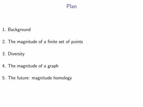
Plan
1. Background
2. The magnitude of a finite set of points
3. Diversity
4. The magnitude of a graph
5. The future: magnitude homology

1. Background
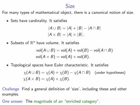
SizeFor many types of mathematical object, there is a canonical notion of size.
• Sets have cardinality. It satisfies
|A ∪ B| = |A|+ |B| − |A ∩ B||A× B| = |A| × |B| .
• Subsets of Rn have volume. It satisfies
vol(A ∪ B) = vol(A) + vol(B)− vol(A ∩ B)
vol(A× B) = vol(A)× vol(B).
• Topological spaces have Euler characteristic. It satisfies
χ(A ∪ B) = χ(A) + χ(B)− χ(A ∩ B) (under hypotheses)
χ(A× B) = χ(A)× χ(B).
Challenge Find a general definition of ‘size’, including these and otherexamples.
One answer The magnitude of an “enriched category”.
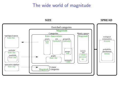
The wide world of magnitude
Metric spaces
associative algebras
orbifolds
graphs
Linearcategories
manifolds
topological spacesEuler char
Euler char
Euler char
Euler char
groups
monoids
convexsets
order
volumeperimeter
CategoriesMagnitude
Magnitude
Enriched categoriesMagnitude
etc.
ecologicalcommunities
diversity
probabilitydistributions
entropy
SIZE SPREAD
order
Euler char
Euler characteristic
charEulerposets
cardinalitysets
cardinalitygroupoids
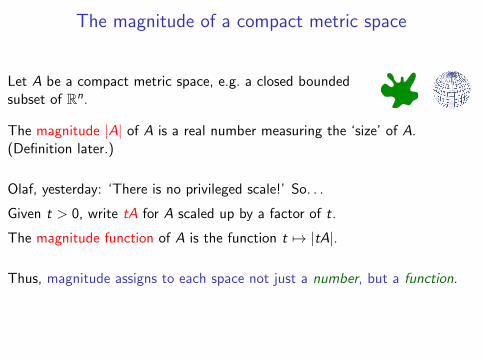
The magnitude of a compact metric space
Let A be a compact metric space, e.g. a closed boundedsubset of Rn.
The magnitude |A| of A is a real number measuring the ‘size’ of A.(Definition later.)
Olaf, yesterday: ‘There is no privileged scale!’ So. . .
Given t > 0, write tA for A scaled up by a factor of t.
The magnitude function of A is the function t 7→ |tA|.
Thus, magnitude assigns to each space not just a number, but a function.
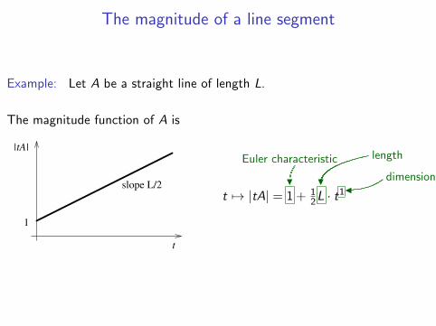
The magnitude of a line segment
Example: Let A be a straight line of length L.
The magnitude function of A is
t
|tA|
1
slope L/2t 7→ |tA| = 1
H
Euler characteristic
+ 12LH
length
· t1Jdimension
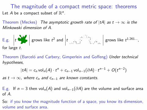
The magnitude of a compact metric space: theoremsLet A be a compact subset of Rn.
Theorem (Meckes) The asymptotic growth rate of |tA| as t →∞ is theMinkowski dimension of A.
E.g.
∣∣∣∣t ∣∣∣∣ grows like t2 and
∣∣∣∣t ∣∣∣∣ grows like t1.261...,
for large t.
Theorem (Barcelo and Carbery; Gimperlein and Goffeng) Under technicalhypotheses,
|tA| = cn voln(A) · tn + cn−1 voln−1(∂A) · tn−1 + O(tn−2)
as t →∞, where cn and cn−1 are known constants.
E.g. If n = 3 then voln(A) and voln−1(∂A) are the volume and surface areaof A.
So: if you know the magnitude function of a space, you know its dimension,volume and surface area.

The magnitude of a compact metric space: theorems
Theorem (Willerton) Let A be a homogeneous Riemannian n-manifold.Then
|tA| = Cn voln(A) · tn + Cn−2TotalScalarCurvature(A) · tn−2 + O(tn−4)
as t →∞, where Cn and Cn−2 are known constants. In particular, whenn = 2,
|tA| = 12πarea(A) · t2 + χ(A) + O(t−2).
Theorem (Barcelo and Carbery) The magnitude of an odd-dimensionalEuclidean ball is a rational function of its radius. Specifically:∣∣tB1
∣∣ = 1 + t,∣∣tB3∣∣ =
1
3!(6 + 12t + 6t2 + t3),∣∣tB5
∣∣ =1
5!
360 + 1080t + 525t2 + 135t4 + 18t5 + t6
3 + t.

The moral
For geometrically interesting subsets of Rn, the magnitude function conveysgeometrically interesting information.
(Despite—or because of?—its very general, abstract categorical origins.)
What information does the magnitude function contain for finite sets ofpoints?
2. The magnitude of afinite set of points
The definition
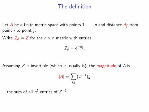
Let A be a finite metric space with points 1, . . . , n and distance dij frompoint i to point j .
Write ZA = Z for the n × n matrix with entries
Zij = e−dij .
Assuming Z is invertible (which it usually is), the magnitude of A is
|A| =∑i ,j
(Z−1)ij
—the sum of all n2 entries of Z−1.
First examples
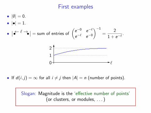
• |∅| = 0.
• |•| = 1.
•∣∣•← `→•
∣∣ = sum of entries of
(e−0 e−`
e−` e−0
)−1=
2
1 + e−`.
0
1
2
`
• If d(i , j) =∞ for all i 6= j then |A| = n (number of points).
Slogan: Magnitude is the ‘effective number of points’(or clusters, or modules, . . . )
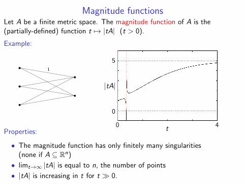
Magnitude functionsLet A be a finite metric space. The magnitude function of A is the(partially-defined) function t 7→ |tA| (t > 0).
Example:
1
|tA|
0
5
t0 4
Properties:
• The magnitude function has only finitely many singularities(none if A ⊆ Rn)
• limt→∞ |tA| is equal to n, the number of points
• |tA| is increasing in t for t � 0.

Detecting clusters at different scales (Willerton)
Magnitude: 1
As the points get further apart, the magnitude gets closer to 3.
Precise version: the magnitude function of the 3-point space
is
Rubinov & Sporns
ObservationMagnitude can be seen as ‘effective number of clusters’, but it’snot always an integer! Awkward reality: ‘clusters’ are ill-defined.
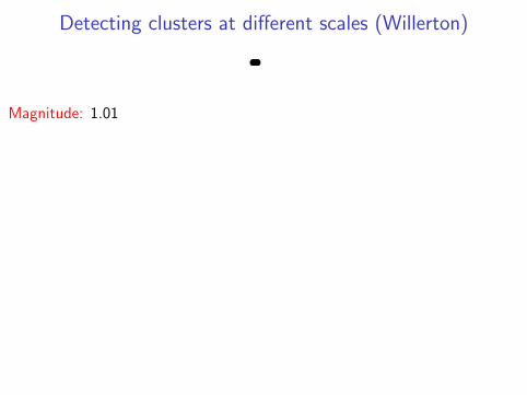
Detecting clusters at different scales (Willerton)
Magnitude: 1.01
As the points get further apart, the magnitude gets closer to 3.
Precise version: the magnitude function of the 3-point space
is
Rubinov & Sporns
ObservationMagnitude can be seen as ‘effective number of clusters’, but it’snot always an integer! Awkward reality: ‘clusters’ are ill-defined.
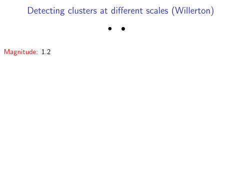
Detecting clusters at different scales (Willerton)
Magnitude: 1.2
As the points get further apart, the magnitude gets closer to 3.
Precise version: the magnitude function of the 3-point space
is
Rubinov & Sporns
ObservationMagnitude can be seen as ‘effective number of clusters’, but it’snot always an integer! Awkward reality: ‘clusters’ are ill-defined.
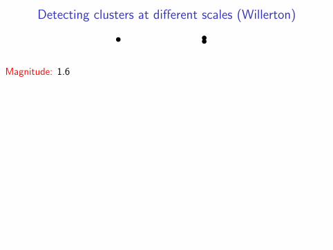
Detecting clusters at different scales (Willerton)
Magnitude: 1.6
As the points get further apart, the magnitude gets closer to 3.
Precise version: the magnitude function of the 3-point space
is
Rubinov & Sporns
ObservationMagnitude can be seen as ‘effective number of clusters’, but it’snot always an integer! Awkward reality: ‘clusters’ are ill-defined.

Detecting clusters at different scales (Willerton)
Magnitude: 2.3
As the points get further apart, the magnitude gets closer to 3.
Precise version: the magnitude function of the 3-point space
is
Rubinov & Sporns
ObservationMagnitude can be seen as ‘effective number of clusters’, but it’snot always an integer! Awkward reality: ‘clusters’ are ill-defined.

Detecting the critical nodes and edgesView a graph as a metric space: the points are the nodes, and the distancebetween nodes is the length of a shortest path between them.
whole graph
MAG FUNCN
one edge onleft deleted
(two near-identicalcurves)
bridge deleted
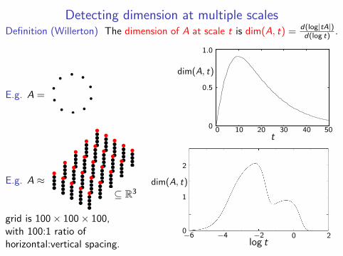
Detecting dimension at multiple scalesDefinition (Willerton) The dimension of A at scale t is dim(A, t) = d(log|tA|)
d(log t) .
E.g. A =
0 10 20 30 40 500
0.5
1.0
t
dim(A, t)
E.g. A ≈⊆ R3
grid is 100× 100× 100,with 100:1 ratio ofhorizontal:vertical spacing.
−6 −4 −2 0 20
1
2
log t
dim(A, t)

An appeal
The only ‘results’ we have on the ability of magnitude functions to detectfeatures of data-sets are a handful of specific examples. We need:
1. More empirical exploration
2. Theorems. . . or at least, conjectures!
Back to compact spaces
There are several equivalent ways to define the magnitude of a compactmetric space X (assuming a technical hypothesis).
The simplest:|X | = sup
{|A| : finite A ⊆ X
}.
With this definition, and lots of analysis, we get all the results on geometricinvariants stated earlier.

3. Diversity
Joint with Christina Cobbold (Ecology, 2012)
A brief history of diversity measurement
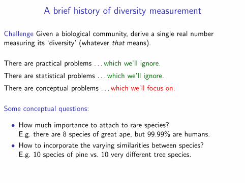
Challenge Given a biological community, derive a single real numbermeasuring its ‘diversity’ (whatever that means).
There are practical problems . . . which we’ll ignore.
There are statistical problems . . . which we’ll ignore.
There are conceptual problems . . . which we’ll focus on.
Some conceptual questions:
• How much importance to attach to rare species?E.g. there are 8 species of great ape, but 99.99% are humans.
• How to incorporate the varying similarities between species?E.g. 10 species of pine vs. 10 very different tree species.

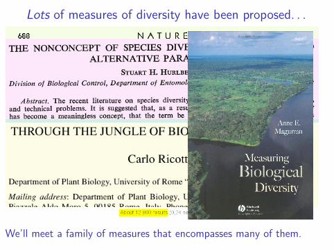
Lots of measures of diversity have been proposed. . .
We’ll meet a family of measures that encompasses many of them.

Lots of measures of diversity have been proposed. . .
We’ll meet a family of measures that encompasses many of them.
Lots of measures of diversity have been proposed. . .
We’ll meet a family of measures that encompasses many of them.
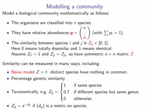
Modelling a communityModel a biological community mathematically as follows:
• The organisms are classified into n species.
• They have relative abundances p =
(p1...pn
)(with
∑pi = 1).
• The similarity between species i and j is Zij ∈ [0, 1].Here 0 means totally dissimilar and 1 means identical.Assume Zii = 1 and Zij = Zji , so have symmetric n × n matrix Z .
Similarity can be measured in many ways, including:
• Naive model Z = I : distinct species have nothing in common.
• Percentage genetic similarity.
• Taxonomically, e.g. Zij =
1 if same species
0.7 if different species but same genus
0 otherwise.
• Zij = e−dij if (dij) is a metric on species.

A unifying family of diversity measures
Recap: We model a community by a relative abundance vector p =
(p1...pn
)and an n × n similarity matrix Z .
• (Zp)i =∑
j Zijpj is the expected similarity between a random organismand one of species i . It measures the ordinariness of species i .
• So 1/(Zp)i is the distinctiveness of species i .
A community is diverse if it contains many distinctive individuals.
So one measure of diversity is the average distinctiveness:∑i
pi1
(Zp)i.
More generally, it’s worth considering the power mean(∑i
pi
(1
(Zp)i
)1−q)1/(1−q)
for every real q (but we’ll stick to q ≥ 0).
A unifying family of diversity measures
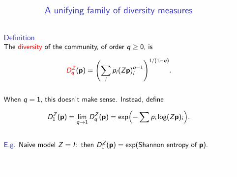
DefinitionThe diversity of the community, of order q ≥ 0, is
DZq (p) =
(∑i
pi (Zp)q−1i
)1/(1−q)
.
When q = 1, this doesn’t make sense. Instead, define
DZ1 (p) = lim
q→1DZq (p) = exp
(−∑
pi log(Zp)i
).
E.g. Naive model Z = I : then DZ1 (p) = exp(Shannon entropy of p).

Properties of these diversity measures
• This family of diversity measures encompassesmany of the measures already defined and used byecologists, geneticists, etc.
• They behave sensibly when species are reclassified(don’t jump suddenly).
• They behave smoothly under change of resolution(e.g. if we go down to the subspecies level).
• They can be used in situations where we don’thave species classifications at all (often the casefor microbial communities).
Influenza strains,1968–2002
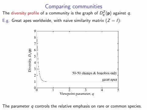
Comparing communitiesThe diversity profile of a community is the graph of DZ
q (p) against q.
E.g. Great apes worldwide, with naive similarity matrix (Z = I ):
The parameter q controls the relative emphasis on rare or common species.
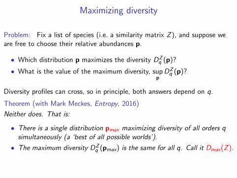
Maximizing diversity
Problem: Fix a list of species (i.e. a similarity matrix Z ), and suppose weare free to choose their relative abundances p.
• Which distribution p maximizes the diversity DZq (p)?
• What is the value of the maximum diversity, supp
DZq (p)?
Diversity profiles can cross, so in principle, both answers depend on q.
Theorem (with Mark Meckes, Entropy, 2016)
Neither does. That is:
• There is a single distribution pmax maximizing diversity of all orders qsimultaneously (a ‘best of all possible worlds’).
• The maximum diversity DZq (pmax) is the same for all q. Call it Dmax(Z ).
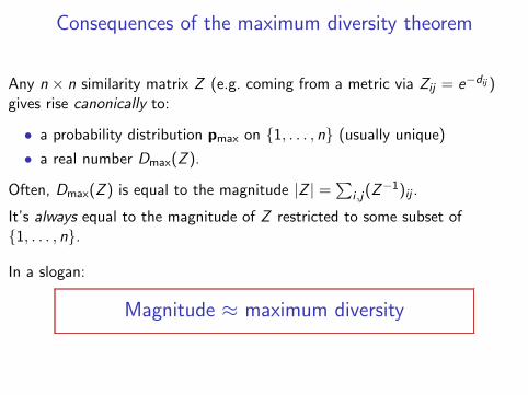
Consequences of the maximum diversity theorem
Any n × n similarity matrix Z (e.g. coming from a metric via Zij = e−dij )gives rise canonically to:
• a probability distribution pmax on {1, . . . , n} (usually unique)
• a real number Dmax(Z ).
Often, Dmax(Z ) is equal to the magnitude |Z | =∑
i ,j(Z−1)ij .
It’s always equal to the magnitude of Z restricted to some subset of{1, . . . , n}.
In a slogan:
Magnitude ≈ maximum diversity
4. Graphs, revisited (briefly)
The magnitude of a graph
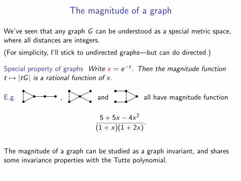
We’ve seen that any graph G can be understood as a special metric space,where all distances are integers.
(For simplicity, I’ll stick to undirected graphs—but can do directed.)
Special property of graphs Write x = e−t . Then the magnitude functiont 7→ |tG | is a rational function of x.
E.g. , and all have magnitude function
5 + 5x − 4x2
(1 + x)(1 + 2x).
The magnitude of a graph can be studied as a graph invariant, and sharessome invariance properties with the Tutte polynomial.

The magnitude of a graphLemma The magnitude function of a graph can also be expressed as apower series with integer coefficients.
E.g. , and have magnitude function
5− 10x + 16x2 − 28x3 + 52x4 − 100x5 + · · · .
In general, the magnitude function of a graph G is
c0 + c1x + c2x2 + · · ·where
c0 = number of nodes
c1 = −2 · (number of edges)
c2 =∑
i ,j :dij=2
((num of configurations i—•—j)− 1
)︸ ︷︷ ︸
redundancy
+ 6 · (num of triangles) + 2 · (num of edges).
5. The future:magnitude homology

Two points of view on Euler characteristic
So far: Euler characteristic has been treated as an analogue of cardinality.
Alternatively: Given any homology theory H∗ of any kind of object X ,can define
χ(X ) =∞∑n=0
(−1)n rank Hn(X ).
Note:
• χ(X ) is a number
• H∗(X ) is an algebraic structure, and functorial in X .
In this sense, homology improves on (“categorifies”) Euler characteristic.
The magnitude homology of a graph (Hepworth–Willerton)
There is a definition (omitted) of the magnitude homology of a graph.
It is a graded homology theory. That is, for each graph G and integer k ≥ 0,it gives a sequence
Hk,0(G ),Hk,1(G ),Hk,2(G ), . . .
of abelian groups.
So for each k ≥ 0, we have a power series
rank(Hk,0(G )) + rank(Hk,1(G ))x + rank(Hk,2(G ))x2 + · · ·
The Euler characteristic χ(G ) for this homology theory is (inevitably) definedas the alternating sum of these power series over k = 0, 1, . . ..
Theorem (Hepworth, Willerton)χ(G ) is exactly the magnitude function of G.
So: magnitude is the Euler characteristic of magnitude homology.
The magnitude homology of a metric space
The definition of magnitude homology can be generalized from graphs toenriched categories (Shulman).
In particular, there is a magnitude homology of metric spaces.
Sample Theorem For a closed set A ⊆ Rn,
A is convex ⇐⇒ H1(A) = 0.
Otter (2018) has done a comparison of magnitude homology with persistenthomology:
• She proves a relationship between persistent homology and a ‘blurredversion’ of magnitude homology. . .
• but concludes that ‘morally, these are very different homology theories’,conveying different information.

Summary

SummaryMagnitude is a numerical invariant of metric spaces (e.g. data sets, networks,and the kinds of space that geometers like thinking about).
By considering rescalings, magnitude assigns a function to each space.
• For geometrically interesting spaces, the magnitude function carriesgeometrically interesting information (volume, dimension, etc).
• For finite spaces, it seems—empirically—to carry multiscale informationon number of clusters and dimensionality.
We can also measure the diversity (∼ entropy) of any probability distributionon a finite metric space. . .
. . . and magnitude is closely related to maximum diversity.
There is a theory of magnitude homology for metric spaces.
It is related to persistent homology, but expresses different information aboutthe space. . . Lots to explore here!
References and further reading: www.maths.ed.ac.uk/∼tl/magbib


![Index [ifers.org]ifers.org/uploads/3/4/9/2/34924997/music_index.pdf255 Index 2D-FMC See 2-dimensional Fourier Magnitude Coefficients, 179 2-dimensional Fourier Magnitude Coefficients,](https://static.fdocument.org/doc/165x107/61174f297a49a9080460fd0e/index-ifersorgifersorguploads349234924997musicindexpdf-255-index-2d-fmc.jpg)